Improving integrated surface water–groundwater modelling with groundwater extraction for water management

ABSTRACT

The purpose of this study is to improve a simultaneous simulation of surface water and groundwater regimes with groundwater extraction to assess the implications for water management and propose primary solution approaches. The SWAT-MODFLOW model is performed for the Yom and Nan river basins during 2007–2016. The results demonstrate that the model provides an accurate depiction of the streamflow and groundwater heads when groundwater pumping is included. The recharges of surface water and groundwater are 2 times higher than the annual average value in the wet year (2011), whereas they are 3 times below the annual average in the dry year (2015). The downstream of Yom River basin is vulnerable to flooding, while high-terrain areas in Nan River basin are vulnerable to drought events. Capturing surplus water volumes during the wet season by recharging into the aquifer, coupled with improving the river capacity and forest areas, should be a sustainable solution for these issues.

KEYWORDS:

• hydrological model
• surface water–groundwater interaction
• SWAT-MODFLOW
• flood
• drought

Editor A. Fiori Associate Editor C. Abesser

Introduction

The global water demand is increasing continuously due to population growth. However, in future decades, changes in climatic patterns and associated hydrological fluxes may cause a decrease in water supply in certain regions (Achieng et al. 2015). Consequently, water management planning must be implemented systematically for sustainable future water supply (Chunn et al. 2019). Providing estimates of available surface water and groundwater and their interaction is an important factor in utilizing water resources effectively and avoiding conflicts of water use in the future (Winter 1995, Sophocleous 2002, Malcolm et al. 2003, Hu et al. 2016).

Certain developing nations, such as Thailand, rely on agricultural exports as a main component of national revenue. However, in recent years, irrigation water volumes in Thailand have increased significantly due to augmented dry seasons (Petpongpan et al. 2021). This increased water usage imposes a significant stress on the nation’s overall water supply, and jeopardizes the government’s strategic water management plans to ensure freshwater supply for domestic, industrial, and agricultural uses (Apipattanavis et al. 2018). Even with governmental policies emphasizing systematic water management for holding a population growth, surface water supplies are insufficient to cover irrigation demand. Therefore, conjunctive water use of all water sources, i.e. surface water and groundwater, is considered a major national priority to optimize water availability for various stakeholders. Conjunctive use of surface water and groundwater in certain regions of Thailand has been assessed in response to the increase in water consumption (Bejranonda et al. 2007). However, the assessment of the hydrological component in Thailand has concentrated on surface water, by not completely integrating with groundwater analyses, or has focused mainly on small watersheds. Thus, a study of coupled, integrated surface water and groundwater regimes in large-scale watersheds for water management would play an important role in the sustainable development of water resources in Thailand.

Generally, water resources management has focused on either surface water or groundwater (Joo et al. 2018), although often they are linked (Dowlatabadi and Zomorodian 2015) via groundwater–surface water interactions along rivers, lakes, and reservoirs. Available volumes of both surface water and groundwater must be assessed to provide optimal water planning and management. Therefore, to achieve a realistic hydrological simulation for supporting conjunctive water use management, surface water and groundwater should be modelled and estimated concurrently instead of being considered individually. Among numerous approaches, often the most appropriate method is the construction of hydrological models that simulate the generation and flow of surface water and groundwater and their interactions (Cho et al. 2010, Bejranonda et al. 2011, Li et al. 2016, Wu et al. 2018).

Many models have been developed in recent decades and applied to watershed management (Sophocleous et al. 1999, Sudicky et al. 2008, Kollet et al. 2016), several of which have coupled the popular watershed and groundwater flow models SWAT (Soil and Water Assessment Tool) and MODFLOW, together called SWAT-MODFLOW (Sophocleous and Perkins 2000, Kim et al. 2008, Bailey et al. 2016). The recharge rate and evapotranspiration of groundwater are estimated in a spatial-temporal distribution according to the hydrological response units (HRUs) of SWAT, while the exchange between river and aquifer occurs along SWAT’s sub-basin streams. This provides advantages for the simulation of long-term impacts such as irrigation management, land-use change, and the effects of climate change (Playan and Mateos 2006, Chu et al. 2013, Guzman et al. 2015).

The most widely used version of SWAT-MODFLOW is that of Bailey et al. (2016), which has been applied to watersheds around the world in recent years (Aliyari et al. 2019, Chunn et al. 2019, Gao et al. 2019, Molina-Navarro et al. 2019, Semiromi and Koch 2019, Wei and Bailey 2019). For this version of SWAT-MODFLOW, two graphical user interface (GUI) platforms have been created to facilitate linkage between the two models and decrease preparation time and pre-processing errors. SWATMOD-Prep (Bailey et al. 2017) is a Python-based stand-alone GUI that creates a single-layer MODFLOW model and links it with an existing SWAT model. QSWATMOD (Park et al. 2019) is a QGIS plug-in tool that interacts with the canvas of QGIS, allowing the user to view maps of SWAT and MODFLOW inputs and view simulation results. An integrated SWAT-MODFLOW model, created by QSWATMOD, is suitable for simulating conjunctive surface water and groundwater regimes in the vulnerable watersheds of Thailand.

This study aims to understand the spatial and temporal variability in water fluxes in different hydrological/hydrogeological compartments within the two study watersheds, and to highlight the areas at risk of extreme flood/drought during different climatic conditions. The study areas are economically crucial agricultural areas in Thailand, namely the Yom and Nan river basins. However, this area appears to be vulnerable to severe hydroclimatic events, as it has seen extreme flood and drought events in many years, including 2011 and 2015, respectively. The coupled simulation of SWAT-MODFLOW (Bailey et al. 2016) is performed using QSWATMOD. In contrast with Petpongpan et al. (2020), the spatial variation in aquifer properties (hydraulic conductivity, specific storage, and specific yield), considered in this study, for spatial hydrological variability inherent in SWAT calculations, are based on the hydrogeological unit field data. Furthermore, the monthly groundwater pumping is taken into account in representing the water irrigation section; in addition, water fluxes in the extreme flood and drought event years are investigated. The results have implications for water management in different climate years, including the appropriate water management approaches for each area.

Material and methods

SWAT-MODFLOW and QSWATMOD

The SWAT-MODFLOW modelling code used in this study (Bailey et al. 2016) is a fully coupled SWAT (Arnold et al. 1998) and MODFLOW-NWT model. SWAT is a physically based, quasi-distributed model, which uses the water balance principle for hydrological process simulation. In the simulation, the model separates the watershed area into two major divisions, namely the land phase and the river phase. The land phase is used to analyse the volume of water loading to the river from each part of the sub-basin via the hydrological pathways of surface runoff, soil lateral flow, and groundwater flow, following Equation (1)(1) $S{W}_t=S{W}_0+\sum _{i=1}^0\left(P-Q_{\mathrm{L}\mathrm{a}\mathrm{n}\mathrm{d}}-E-W-Q_{\mathrm{g}\mathrm{w}}\right)$(1) . Meanwhile, the river phase is the movement of water through the stream network to the outlet of the sub-basin, represented by Manning’s equation (Equation 2(2) $Q_{\mathrm{R}\mathrm{i}\mathrm{v}\mathrm{e}\mathrm{r}}=\frac{A\times R^{2/3}\times s^{1/2}}{n}$(2) ) and the Muskingum River routing method (Equation 3(3) $Q_{\mathrm{o}\mathrm{u}\mathrm{t},2}=c_1.Q_{\mathrm{i}\mathrm{n},2}+c_2.Q_{\mathrm{i}\mathrm{n},1}+c_3.Q_{\mathrm{o}\mathrm{u}\mathrm{t},1}$(3) ) (Arnold et al. 1998, 2012, Neitsch et al. 2011).

(1) $S{W}_t=S{W}_0+\sum _{i=1}^0\left(P-Q_{\mathrm{L}\mathrm{a}\mathrm{n}\mathrm{d}}-E-W-Q_{\mathrm{g}\mathrm{w}}\right)$(1)

(2) $Q_{\mathrm{R}\mathrm{i}\mathrm{v}\mathrm{e}\mathrm{r}}=\frac{A\times R^{2/3}\times s^{1/2}}{n}$(2)

(3) $Q_{\mathrm{o}\mathrm{u}\mathrm{t},2}=c_1.Q_{\mathrm{i}\mathrm{n},2}+c_2.Q_{\mathrm{i}\mathrm{n},1}+c_3.Q_{\mathrm{o}\mathrm{u}\mathrm{t},1}$(3)

where SW₀ is the water content of the soil on the first day (mm), SW_t is the water content of the soil on the last day (mm), P is the amount of precipitation on day i (mm), Q_Land is the surface runoff on day i (mm), Q_River is the river runoff on day i (mm), E is the amount of evapotranspiration on day i (mm), W is the percolation through the lower soil profile on day i (mm), Q_gw is the volume of water recharge on day i (mm), A is the channel cross-section (m²), R is the hydraulic radius (m), S is the channel slope length, n is the Manning’s coefficient of the river channel, Q_in,1 is the inflow rate at the first time step (m³/s), Q_in,2 is the inflow rate at the last time step (m³/s), Q_out,1 is the outflow rate at the first time step (m³/s), Q_out,2 is the outflow rate at the last time step (m³/s), and C is the Muskingum coefficient.

MODFLOW solves the groundwater flow equation by discretizing the aquifer into grid cells, having nodes at the centre of the cell for calculation. The position of grid cells is defined in terms of rows, columns, and layers. To simulate the groundwater head in each cell and, subsequently, the change of head in each cell in transient simulations, a finite difference approximation (i.e. a water balance equation) is formulated for each grid cell based on the continuity equation, as shown in Equation (4)(4) $\frac{\mathrm{\Delta }h}{\mathrm{\Delta }t}{S}_s\mathrm{\Delta }V=\sum Q_{\mathrm{s}\mathrm{o}\mathrm{u}\mathrm{r}\mathrm{c}\mathrm{e}}-\sum Q_{\mathrm{s}\mathrm{i}\mathrm{n}\mathrm{k}}+\frac{\mathrm{\partial }{Q}_{\mathrm{i},\mathrm{j},\mathrm{k}}}{\mathrm{\partial }x}+\frac{\mathrm{\partial }{Q}_{\mathrm{i},\mathrm{j},\mathrm{k}}}{\mathrm{\partial }y}+\frac{\mathrm{\partial }{Q}_{\mathrm{i},\mathrm{j},\mathrm{k}}}{\mathrm{\partial }z}$(4) :

(4) $\frac{\mathrm{\Delta }h}{\mathrm{\Delta }t}{S}_s\mathrm{\Delta }V=\sum Q_{\mathrm{s}\mathrm{o}\mathrm{u}\mathrm{r}\mathrm{c}\mathrm{e}}-\sum Q_{\mathrm{s}\mathrm{i}\mathrm{n}\mathrm{k}}+\frac{\mathrm{\partial }{Q}_{\mathrm{i},\mathrm{j},\mathrm{k}}}{\mathrm{\partial }x}+\frac{\mathrm{\partial }{Q}_{\mathrm{i},\mathrm{j},\mathrm{k}}}{\mathrm{\partial }y}+\frac{\mathrm{\partial }{Q}_{\mathrm{i},\mathrm{j},\mathrm{k}}}{\mathrm{\partial }z}$(4)

where Q_source is the flow rate (m³/d) of a source of groundwater to the aquifer (e.g. recharge, stream seepage), Q_sink is the rate of groundwater removal (m³/d) from the aquifer (e.g. pumping, groundwater discharge to streams, groundwater ET), S_s is the specific storage (m⁻¹), ∆V is the volume of the grid cell (m³), and ∆h is the change in water head (m) over the time interval ∆t (d). For unconfined aquifers, the specific yield (S_y) is used as the storage property.

The linkage process of SWAT-MODFLOW is presented in Fig. 1. It is operated via the HRU and sub-basin based variables of the SWAT model and cell-based variables of the MODFLOW model. The hydrological regime of the land phase is simulated by the SWAT model and transferred to the MODFLOW’s grid in terms of the stream stage and water percolation (i.e. recharge). The percolation from the SWAT model is mapped to the Recharge package of MODFLOW model to specify the groundwater recharge volume. Then, the groundwater head for each grid cell, and the surface water and groundwater interaction exchange rates for each river cell along the SWAT sub-basin streams, is estimated using Darcy’s Law. This latter calculation uses streambed conductivity, streambed thickness, the length of the stream in the cell, and the stream width to calculate the flow between the aquifer and the stream via the streambed. Groundwater discharge to the stream occurs if the groundwater head in the cell is higher than the river stage; stream seepage to the aquifer occurs if the river stage is higher than the groundwater head. The resulting rate of exchange between the river and aquifer is passed to the associated SWAT sub-basin stream for stream routing (Bailey et al. 2016). When the SWAT-MODFLOW is used, the original groundwater module of SWAT is deactivated.

Figure 1. Linkage process between SWAT and MODFLOW in the SWAT-MODFLOW modelling code (Bailey et al. 2016)

Study area

The Yom and Nan river basins are important agricultural regions located in the north of Thailand (Fig. 2) and cover 37% (58 800 km²) of the Chao Phraya River basin. This region is defined as a crucial source of agriculture and travel of Thailand, producing a significant portion of the country’s annual income. Unfortunately, extreme flood and drought events occur frequently, especially in the downstream area, causing widespread damage. The Yom River basin starts at the high mountain area and flows through the steep valley into the middle of the watershed, which is mostly characterized by narrow plains areas and terraced mountains. In the upper part of the basin, the large majority of the area is forest and agriculture, whereas in the lower part, the topography is dominated by plains areas. The forested and agricultural areas are reduced due to urban expansion. The average annual rainfall is 1150 mm, causing an average annual runoff of 5000 × 10⁶ m³. Most rainfall occurs during the wet season between May and October due to the influence of the tropical depression, Southwest monsoon, and Northwest monsoon from the South China Sea (Hydro and Agro Informatics Institute 2012).

Figure 2. Location of Yom and Nan river basins including the runoff stations, groundwater observation wells, rainfall stations, weather stations, and Sirikit Dam in the study area

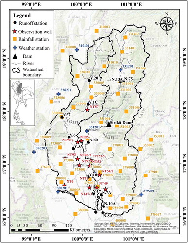
The Nan River basin begins at the Luang Prabang Mountains, which form the Thailand-Laos border, and flows through plains between valley areas into the Sirikit Dam. Historically, this valley was an abundant source of water for the Nan River because of many river branches and large forested areas. Recently, however, the forested areas have been reduced for corn cultivation, affecting the hydrological processes and water quality of the area. In the lower part, the Nan River flows parallel to the Yom River, before they converge at the flat plains area. The annual rainfall and runoff are about 1300 mm and 12 000 × 10⁶ m³, respectively. Approximately 80% of the available water is used for agriculture. Similar to the Yom River basin, 85% of rainfall occurs during July and September, as a result of a tropical depression and monsoon from the South China Sea (Hydro and Agro Informatics Institute 2012).

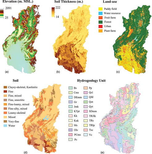
Figure 3(a) shows that the highest elevation of the ground surface is approximately 2090 m (MSL) in the upstream mountain area in the watershed, whereas the lowest elevation is 25 m (MSL) in the downstream plains. The thickness of the alluvial aquifer (Fig. 3(b)) ranges from 14 m in the mountain areas to 222 m in the plains areas. As shown in Fig. 3(c) and (d), almost 60% of the watershed is forest, followed by paddy fields (20%) and plant farms or horticulture (11%), while urban land use is the lowest at 3%. Half of the watershed area is mixed soil, comprising various soil types in upstream forest areas. The downstream plains areas are mainly fine mixed soil (11%) and fine-silty mixed soil (8%). Regarding the aquifer (Fig. 3(e)), high-terrain areas, especially the upstream rea, are consolidated aquifers and Tertiary semi-consolidated aquifer, accounting for 55% and 5% of the watershed area, respectively. Downstream plains areas consist of unconsolidated aquifers, which account for about 40% of the watershed area.

Figure 3. Topography dataset of the study area: (a) digital elevation model, (b) soil thickness, (c) land use, (d) soil, and (e) aquifer

Method

Data collection

Simulating the surface water and groundwater regimes with the SWAT-MODFLOW model requires sets of topography data and hydrometeorological data. In this study, the topography of the study area is generated by defining the digital elevation model (DEM) and spatial soil depth data as ground surface elevation and aquifer thickness, respectively. The 90 m resolution DEM data are collected from the Shuttle Radar Topography Mission (SRTM), while the 1 km resolution soil depth grid data can be accessed via the global gridded soil information of the International Soil Reference and Information Centre (ISRIC). Land-use data and soil data are provided by the Land Development Department (LDD) and Department of Mineral Resources (DMR), respectively, by which they are processed into 90 m resolution grid data.

The hydrometeorological data are time-series data, consisting of weather conditions (see details below), river discharge, groundwater level, and reservoir operation (see details below). The meteorological data, used in this study to define the weather conditions of the Yom and Nan river basins, are precipitation, maximum and minimum air temperature, dew point temperature, wind speed, humidity, and solar radiation. These data are collected from 43 rainfall stations and 10 weather stations of the Thai Meteorological Department (TMD) (see station locations and code names in Fig. 2). Only rainfall data are considered on a daily scale, while the others are monthly because of data availability. Reservoir operation data comprise daily outflow release and storage information of the Sirikit Dam, located in the Nan River (see Fig. 2 for location) from the Electricity Generating Authority of Thailand (EGAT). Monthly pumping volumes are from 6152 groundwater pumping wells of the Department of Groundwater Resources (DGR), located principally in the downstream (plains) areas of the river basins. Their locations cannot be shown on the map in Fig. 2 due to their large number. The model is calibrated and validated by comparing the simulated river discharges and groundwater heads to the observation data. River discharge is measured daily from 15 runoff stations of the Royal Irrigation Department (RID), while groundwater head is measured monthly from 14 groundwater observation wells of the DGR (Fig. 2). The additional information from the runoff stations and observation wells is provided in Tables 1 and 2, respectively.

Table 1. Details of the runoff stations

Stations	Coordinates		Catchment area (km^2)	Elevation (m MSL)	Period of available records
	UTM E (m)	UTM N (m)
Y.20	621 852	2 055 046	5394	193.552	1971 to present
Y.1 C	619 313	2 005 048	7749	153.972	1979 to present
Y.37	564 342	1 978 481	10 305	105.250	1999 to present
Y.6	584 054	1 927 663	12 769	68.928	1952 to present
Y.3A	588 044	1 913 663	13 331	65.350	1967 to present
Y.16	619 465	1 852 884	20 201	43.630	1967 to present
Y.17	628 799	1 825 224	22 034	41.843	1967 to present
Y.5	635 058	1 779 493	24 046	32.000	1967–2012
N.75	704 513	2 100 956	2170	196.616	2006 to present
N.13A	686 465	2 052 151	8706	192.700	1987 to present
N.60	620 322	1 925 666	18 447	57.592	1986 to present
N.7A	642 488	1 820 973	27 897	37.143	2000 to present
N.10A	651 439	1 792 732	30 328	33.300	1969 to present
N.8A	649 721	1 778 060	31 472	30.978	2000 to present

Table 2. Details of the observation wells

Name code	Coordinates		Aquifer layer	Elevation (m MSL)	Drilling depth (m)	Normal GW level (m)
	UTM E (m)	UTM N (m)
NT47/3	620 234	1 834 058	Qyt	44	70	10
NT48/2	651 533	1 829 785	Qyt	44	130	16
NT49	637 182	1 831 748	Qfd	48	80	12
NT51	615 891	1 842 061	Qyt	45	80	10
NT52	622 612	1 876 954	Qyt	46	60	10
NT53/3	624 936	1 888 352	Qfd	52	64	26
NT54/2	642 743	1 857 853	Qfd	45	70	12
NT6	569 092	1 835 860	Qyt	65	58	3.5
NT92	600 433	1 878 172	Qyt	52	94	15
NT93	570 333	1 892 280	Qyt	65	110	3.2
NT95	604 572	1 928 890	Qyt	58	90	14.76
NT96/3	596 812	1 891 238	Qyt	51	70	18
NT99/2	597 171	1 926 367	Qyt	59	65	15
NT57	619 492	1 997 577	Qyt	164	45	3

SWAT-MODFLOW application

The SWAT-MODFLOW simulation spans the time period 2004–2016 at a daily time step. The first 3 years (2004–2006) were defined as a warm-up period. ArcSWAT2012 was used to prepare SWAT input files from the hydrological, soil, topography, and land-use datasets. The sub-basins and stream reaches of the watershed were generated based on the DEM. The outlets of the Yom and Nan river basins were indicated at the position of stations Y.5 and N.8A, respectively (see Fig. 2), resulting in 111 sub-basins and stream reaches (Fig. 4(a)). The model domain was divided into 2102 HRUs by overlaying each sub-basin with land use and soil type in a 1% ratio definition. The reservoir operation was controlled by the daily water release and storage information of the Sirikit Dam.

Figure 4. (a) Sub-basins and river reaches of Yom and Nan river basins generated by SWAT, and (b) active grid cells and river grid cells of Yom River and Nan River basins generated by MODFLOW

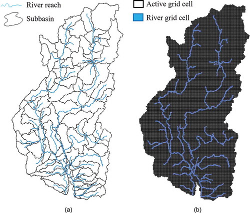
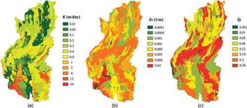
QSWATMOD was used to create the single-layer MODFLOW finite-difference grid, link with SWAT HRUs and sub-basins, create all necessary input files, and run the simulation. The finite-difference grid of MODFLOW was created using the “Set up MODFLOW Grid Size (in map unit)” function in the “Create a Simple MODFLOW model” option (Park and Bailey, 2017). In this study, the grid cells of MODFLOW were defined at a resolution of 900 m for a single layer, resulting in 108 927 grid cell numbers. Table 3 provides the SWAT parameters which are varied manually for a simulation of surface water and groundwater in the Yom and Nan river basins. Figure 4(b) shows MODFLOW’s active grid cells and 3906 river cells, with the latter obtained by intersecting the grid with SWAT’s river network shapefile. During the linkage process, SWAT HRUs were separated spatially into 308 188 disaggregated HRUs (DHRUs). Aquifer thickness (see Fig. 3(b)), hydraulic conductivity (K), specific storage (S_s), and specific yield (S_y) were loaded as raster files into QSWATMOD, with K, S_s, and S_y varied spatially (Fig. 5) according to the aquifer types. The values for K range between 0.01 and 24 m/d, while ranges for S_s and S_y are 0.0001–0.02 m⁻¹ and 0.001–0.26, respectively. Groundwater pumping volumes were included in MODFLOW, with rates only applied for the irrigation season of November to April of each year. In the implementation process, the groundwater abstraction module was included in this simulation by adding an activation source code to the Name file of MODFLOW-NWT (*.nam), then creating the groundwater pumping rate input file for the Well package (*.wel) and defining a time interval as monthly for transient simulation to the discretization file (*.dis).

Table 3. Calibrated parameters of the SWAT model used in surface water–groundwater simulation for the Yom and Nan river basins

Name	Value	Unit
SCS runoff curve number for moisture condition 2 (CN_2)	28.0–92.8	-
Available water capacity of the soil layer (Sol_AWC)	0.050–0.525	(mm/mm)
Saturated hydraulic conductivity (Sol_K)	0.3–150.0	(mm/h)
Soil evaporation compensation factor (ESCO)	0.40–0.95	-
Manning’s “n” value for the tributary channels (CH_N1)	0.014–0.150	-
Effective hydraulic conductivity in tributary channel alluvium (CH_K1)	0–40	(mm/h)
Manning’s “n” value for the main channel (CH_N2)	0.014–0.250	-
Effective hydraulic conductivity in main channel alluvium (CH_K2)	0–30	(mm/h)
Baseflow alpha factor (Alpha_BF)	0.048–0.100	(d)

Figure 5. Spatial distribution of aquifer parameters used in surface water–groundwater simulation for the Yom and Nan river basins, namely (a) hydraulic conductivity (K), (b) specific storage (S_s), and (c) specific yield (S_y)

Investigation of model performance

The simulated river discharges and groundwater heads at the stream gauges and observation wells were used to calibrate and validate the model over the periods 2007–2011 and 2012–2016, respectively. The concordance between the simulation and observation values is assessed using statistical comparison indices – Nash-Sutcliffe efficiency (NSE), coefficient of determination (R²), and percent bias (PBIAS) – which can be computed following Equations (5)(5) $\mathrm{N}\mathrm{S}\mathrm{E}=1-\frac{{\sum }_{i=1}^n{(X_i^{\prime }-X_i)}^2}{{\sum }_{i=1}^n{(X_i-\bar{X})}^2}$(5) –(7(7) $\mathrm{P}\mathrm{B}\mathrm{I}\mathrm{A}\mathrm{S}=\frac{{\sum }_{i=1}^n\left(X_i-X_i^{\prime }\right)}{{\sum }_{i=1}^n\left(X_i\right)}$(7) ), respectively:

(5) $\mathrm{N}\mathrm{S}\mathrm{E}=1-\frac{{\sum }_{i=1}^n{(X_i^{\prime }-X_i)}^2}{{\sum }_{i=1}^n{(X_i-\bar{X})}^2}$(5)

(6) $R^2=\frac{{\sum }_{i=1}^n{(X_i^{\prime }-\bar{X})}^2}{{\sum }_{i=1}^n{(X_i-\bar{X})}^2}$(6)

(7) $\mathrm{P}\mathrm{B}\mathrm{I}\mathrm{A}\mathrm{S}=\frac{{\sum }_{i=1}^n\left(X_i-X_i^{\prime }\right)}{{\sum }_{i=1}^n\left(X_i\right)}$(7)

where $X_i$ and $X_i^{\prime }$ are the observation data and simulated results, respectively, and $\bar{X}$ are the observation data on average. NSE is a normalized statistic, typically applied to reflect the overall fit of continuous hydrograph modelling. It can investigate the relation of observation and simulation data by comparing the observed value with the simulated value and the average observation value. The range of NSE is between −∞ and 1, while values of 0–1 are generally considered an acceptable condition. The parameter R² defines the relation of observation and simulation data using the ratio of the difference between average observation value and simulated/observed value. The range of R² is 0–1. The optimal value for NSE and R², indicating a perfect simulation of the model, is 1. PBIAS is the ratio of deviation from the simulation and observation value. Positive and negative PBIAS values mean the simulated results are underestimated and overestimated, respectively. Thus, the optimal value of PBIAS is 0 (Nash and Sutcliffe 1970, Moriasi et al. 2007).

Scenarios

Following the calibration and validation of the model, a series of scenarios were run to test the model response to changes in climatic conditions, including wet years (extreme flood event) and dry years (extreme drought event). In addition, the impact of groundwater pumping on simulated stream discharge and groundwater levels was investigated.

Results and discussion

Model calibration and validation

The performance of the SWAT-MODFLOW model for the integrated surface water and groundwater system of the Yom and Nan river basins is demonstrated graphically in Figs 6–8, with statistical comparisons presented in Tables 4 and 5. The comparison of daily river discharge at runoff stations Y.1 C, Y.16, N.13A, and N.7A over the period 2007–2016 (Fig. 6), which are representative examples of all stations, shows good agreement between the simulated results and observed data. The annual pumping volume is estimated at 400 × 10⁶ m³, on average, accounting for 2.5% of the river runoff volume.

Table 4. Statistical comparison (NSE, R², and PBIAS) of daily river discharge between the simulated results and observed data in the Yom and Nan river basins

Basin	Station	Calibration (2007–2011)			Validation (2012–2016)
		NSE	R^2	PBIAS (%)	NSE	R^2	PBIAS (%)
Yom	Y.20	0.79	0.79	2.4	0.61	0.62	1.9
	Y.1 C	0.80	0.80	−2.1	0.69	0.69	6.9
	Y.37	0.83	0.83	−5.2	0.74	0.74	6.8
	Y.6	0.76	0.77	4.8	0.71	0.72	11.4
	Y.3A	0.80	0.80	2.4	0.71	0.74	−26.4
	Y.16	0.84	0.87	12.7	0.78	0.81	−28.5
	Y.17	0.78	0.78	−2.6	0.70	0.80	−28.1
	Y.5	0.79	0.80	−0.8	0.81	0.73	−22.7
Nan	N.75	0.79	0.79	3.0	0.76	0.78	11.6
	N.13A	0.79	0.81	10.3	0.83	0.84	14.9
	Inflow of Sirikit Dam	0.79	0.83	−6.4	0.83	0.84	3.3
	N.60	0.83	0.86	9.7	0.80	0.88	12.1
	N.7A	0.83	0.85	7.3	0.70	0.72	−2.2
	N.10A	0.81	0.83	0.0	0.66	0.71	−24.7
	N.8A	0.80	0.84	0.8	0.65	0.71	−19.1

Table 5. Statistical comparison (NSE, R², and PBIAS) of monthly groundwater depth between the simulated results (with and without groundwater pumping) and observed data from all groundwater observation wells during 2007–2016

Simulation scenarios	Calibration (2007–2011)			Validation (2012–2016)
	NSE	R^2	PBIAS (%)	NSE	R^2	PBIAS (%)
with GW pumping	0.80	0.81	−3.8	0.91	0.92	6.6
without GW pumping	0.58	0.68	10.7	−3.14	0.34	80.6

Figure 6. Daily river discharge from the QSWATMOD simulation compared to observation data at runoff stations Y.1 C, Y.16, N.13A, and N.7A during 2007–2016

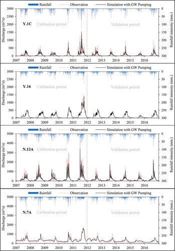
Figure 7. Monthly groundwater elevation from the QSWATMOD simulation with groundwater pumping, compared to a simulation without groundwater pumping and observation data from the groundwater observation wells NT57, NT52, NT99, and NT47 during 2007–2016

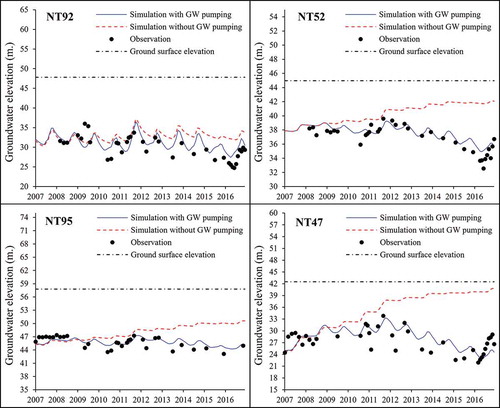
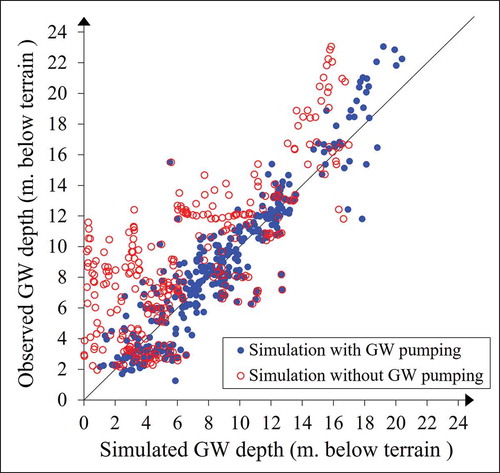
Figure 8. Comparison of monthly groundwater (GW) head between the simulated results (with and without groundwater pumping) and observed data from all groundwater observation wells during 2007–2016

A statistical comparison of the simulation and observation values is presented in Table 4. In the calibration period (2007–2011), the NSE and R² values obtained from all 15 calibrated stations in the Yom and Nan river basins are higher than 0.75. For the Yom River basin, the highest values of NSE and R² were obtained at station Y.16, in the downstream area. The lowest values for both NSE and R² were found at station Y.6, located in the middle of the basin. In the Nan River basin, stations N.60, N.7A, N10A, and N8A, located in the lower part below the Sirikit Dam, show higher NSE and R² values than those obtained in stations N.75 and N13A and at the inflow of the dam in the upstream area. This is because of a defined outflow release of the dam which forces streamflow behaviour in the downstream area, especially in the dry season (November–April). The PBIAS values are in a range of −5.2% to 12.7% for the Yom River basin and −6.4% to 10.3% for the Nan River basin. Based on their positive PBIAS values, the river discharge in the Yom and Nan river basins is mostly underestimated by 0.8–12.7%, except for stations Y.1 C, Y.37, Y17, and Y5 and the inflow of the Sirikit Dam, for which PBIAS values are negative, suggesting that flows are overestimated by 0.8–6.4%. The greatest underestimation is 12.7% at station Y.16 and 10.3% at station N.60 for the Yom and Nan river basins, respectively. For the validation period (2012–2016), in both the Yom and Nan river basins, almost all stations show NSE and R² values greater than 0.65. The PBIAS values are between −28.5% and 14.9%. All stations located in the middle and upper parts of the watershed provide positive PBIAS values, implying that the simulated river discharge in these areas is underestimated by 1.9–14.9%. In contrast, in the lower parts, river discharges are overestimated by 2.2–28.5%, as demonstrated by their negative PBIAS values. The maximum overestimation is 28.5% at station Y.16, while the maximum underestimation is 14.9% at station N.13A.

In general, daily river discharge simulated by the SWAT-MODFLOW model is very consistent with the observation data in both pattern and quantity, whether during the calibration period or the validation period. The simulated results are acceptable and can be classified as “very good” based on the achieved NSE (Moriasi et al. 2007) and R² values. Even the lower values of 0.61 (NSE) and 0.62 (R²) at station Y.20 during the validation period can still be considered “adequate” (Moriasi et al. 2007). In the validation period, daily river discharges in the downstream reaches of both the Yom and Nan river basins are overestimated, even though they are underestimated during the calibration period. This may be due to the effect of calibrating the model to the high discharge rates of the great flood year of 2011. Nevertheless, the simulated daily river discharges obtained in this study represent an improvement over Petpongpan et al. (2020), who simulated surface water and groundwater of the Yom and Nan river basins via the SWATMOD-Prep interface. Despite the difference in the numbers of assessed stations, their study obtained NSE and R² values higher than 0.75 during the calibration period (2007–2011) and higher than 0.60 during the validation period (2012–2016), which is consistent with this study. However, the simulated results of their study are mainly overestimated, especially in the Yom River basin. Most of their stations show a negative PBIAS and the highest value is −35.6%, higher than the present study in which the estimated model error on either of these simulations is in the range of ±30%.

Figures 7 and Figures 8 present a comparison of monthly simulated and observed groundwater heads for simulations with and without groundwater pumping. Examples of simulated results from four groundwater observation wells (Fig. 7) show that using groundwater pumping is more consistent with the observed data than results that exclude them, with the no-pumping scenario overestimating groundwater levels. Monthly groundwater levels from the simulation with groundwater pumping have similar patterns and magnitude of fluctuation to the observed data, likely due to the seasonal drawdown and recovery patterns caused by the pumps operating during the growing season and then being shut off, as well as transpiration in growing and non-growing seasons.

In addition, the simulated and observed groundwater depths from all 14 groundwater observation wells are correlated and represented as a quantile-quantile (Q-Q) plot (Fig. 8) with statistical comparison (Table 5). Results of the simulation including groundwater pumping (blue dots) are considerably closer to the 1:1 line than those of the simulation that excludes groundwater pumping (red dots), which are mostly above the line and provide an overestimation of groundwater heads. The statistical indices of the two simulated scenarios are very different. In the calibration period, NSE and R² for a simulation with groundwater pumping are almost the same at 0.80, but in the simulation without groundwater pumping they are 0.58 and 0.68, respectively. Regarding the PBIAS, the groundwater heads simulated by including groundwater pumping are 3.8% lower than the observation data, on average; without groundwater pumping, PBIAS would be increased 14.5%, accounting for 10.7% overestimation. For the validation period, the NSE and R² values obtained from simulation with groundwater pumping increased to approximately 0.91–0.92. In contrast, without groundwater pumping, the NSE decreased to −3.14, while the R² decreased to 0.34. PBIAS values show a dramatic difference in groundwater heads of both scenarios, which are overestimated by 6.6% and 80.6% when simulated with and without groundwater pumping, respectively.

These results indicate that the application of groundwater pumping has a significant impact on groundwater storage in the aquifer system and is necessary for the accuracy of the model. The simulated results in some locations and periods are different from observed data due to the uncertainties inherent in applying a grid-based model to a large-scale watershed, such as grid cell size or spatial variability of inputs. PBIAS values show a groundwater simulation consistent with the results of Petpongpan et al. (2020) in that the groundwater heads are overestimated in the calibration period and underestimated in the validation period. However, the PBIAS numbers obtained in this study are about twice lower than in their study. Moreover, the NSE and R² values achieved in this study are greater than 0.80 for both calibration and validation periods – higher than those obtained by Petpongpan et al. (2020), which were mainly between 0.71 and 0.80.

Groundwater recharge

The spatial distribution of groundwater recharge per year, for each 900 m × 900 m grid cell area, is illustrated in Fig. 9. On the average, (Fig. 9(a)), about 41% of the watershed area contains groundwater recharge of 200–400 mm. The areas with groundwater recharge of less than 200 mm are equal in proportion to the areas where the groundwater recharge is between 400 and 600 mm, at 25%, while the areas exceeding 600 mm of groundwater recharge account for 9% of the watershed. The upper Yom River basin has annual groundwater recharge higher than 200 mm. In some plains areas it is over 600 mm, whereas the groundwater recharge in the lower area is mostly less than 200 mm.

Figure 9. Spatial groundwater (GW) recharge in the Yom and Nan river basins: (a) average annual (2007–2016); (b) during the wet year (2011); and (c) during the dry year (2015)

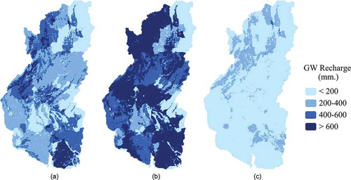
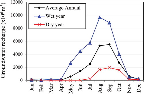
This contrasts with the Nan River basin wherein most of the high groundwater recharge (>400 mm) occurs in the downstream area, especially around the outlet of the basin, while water recharge to the aquifer in the upstream forest and mountain areas is less than 400 mm. In the wet year of 2011 (Fig. 9(b)), the groundwater recharge volume increased significantly. This caused over half of the watershed area (52%) to contain a groundwater recharge greater than 600 mm, which was 43% above the average annual amount. The areas with groundwater recharge of 200–400 mm and 400–600 mm were reduced to 11% and 23%, respectively, while the remaining 14% of the watershed area had groundwater recharge of less than 200 mm. In the dry year of 2015 (Fig. 9(c)), the groundwater recharge in almost the whole watershed area is below 400 mm. About 83% of the area has groundwater recharge of less than 200 mm, while another 16.5% has 200–400 mm. The areas with groundwater recharge between 400 and 600 mm, and higher than 600 mm, are detected in a trivial proportion at 0.5% in total. Referring to Fig. 10, the groundwater recharge is produced during May–October in the average year and wet year, but in the dry year it occurred between August and October. In terms of the annual average, the highest groundwater recharge volume is 5500 × 10⁶ m³ in September. This increased to almost 10 000 × 10⁶ m³ (August) in the wet year and decreased by 3 times to 6000 × 10⁶ m³ (September) in the dry year. In total, there was a groundwater recharge of 18 900 × 10⁶, 36 500 × 10⁶, and 5700 × 10⁶ m³ for the annual average, wet, and dry conditions, respectively.

Figure 10. Monthly groundwater recharge rate in the Yom and Nan river basins: average annual (2007–2016), during the wet year (2011), and during the dry year (2015)

As a consideration, high recharge rates of groundwater occur mainly in the plains areas. The lower part of the watershed, especially the outlet area, shows significant changes in groundwater recharge. There is a large volume of water recharged to the aquifer during the wet year, while the volume decreases dramatically below the annual average in the dry year. The groundwater recharge during the dry year is later than during the average or wet year, by about 3 months for the onset of recharge and 1 month for the peak recharge. This has significant implications for water management, as described below. Moreover, we should note that as observation wells are located only in the downstream areas of each river basin, the simulated groundwater storage in the upstream areas has not been tested. However, as the stream discharge in these areas is simulated accurately, we can assume that groundwater flow is also well simulated.

Surface water–groundwater interactions

Figures 11 and Figures 12 provide the spatial-temporal interactions (e.g. exchange rates) of water between the rivers and the aquifer. Figure 11 presents the quantity of groundwater discharged to the river per year in each river grid cell for the annual average, wet year, and dry year. Negative values indicate the groundwater return flow or river seepage. During 2007–2016, on average (Fig. 11(a)), 48% of each river is recharged by the groundwater to less than 500 mm, while 24% is recharged to 500–1000 mm, and 9% is higher than 1000 mm; 12% of each river is a seepage to the aquifer by less than 500 mm, while 3% is 500–1000 mm, and 4% is higher than 1000 mm. In the wet year of 2011 (Fig. 11(b)), the streams with groundwater discharge to the river of 500–1000 mm and higher than 1000 mm increased by 11% and 20%, respectively, from the average, whereas the ratios of groundwater discharge and river seepage at less than 500 mm were 23% and 5%, respectively, or below the average annual by 24% and 7%. The streams with seepage to the aquifer greater than 500 mm are rather constant. In the dry year of 2015 (Fig. 11(c)), the rivers containing low-magnitude (< 500 mm) recharge from groundwater and seepage to the aquifer are more than 8% of the annual average, at 55% and 20%, respectively. The share of streams with groundwater discharge greater than 500 mm is 19%, which is 14% below the average annual. Meanwhile, the streams with river seepage greater than 500 mm are 5% (2% less than the average annual).

Figure 11. Groundwater discharge from the aquifer to the river in the Yom and Nan river basins: (a) average annual (2007–2016); (b) during the wet year (2011); and (c) during the dry year (2015)

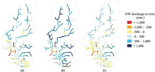
Figure 12. Monthly recharge of the surface water (SW) and groundwater (GW) with various components, consisting of the surface runoff to streams (surq), lateral flow to streams (latq), groundwater flow to streams (gwq), water percolation to groundwater (perco), and river seepage to the aquifer (swgw): (a) average annual (2007–2016); (b) during a wet year (2011); and (c) during a dry year (2015)

There is about 230 × 10⁶ m³ of groundwater discharge to the river per year, on average, while the river seepage to the aquifer is estimated at 40 × 10⁶ m³. The volume of groundwater flowing to the river increased to 310 × 10⁶ m³ in the wet year (2011) due to an increased groundwater recharge from water percolation, and therefore a rising groundwater gradient towards the river reaches, whereas it decreased to 200 × 10⁶ m³ in the dry year (2015). The river seepage is approximately 80 × 10⁶ m³ in the wet year and 20 × 10⁶ m³ in the dry year. It can be noted that, in the wet year, the proportion of groundwater discharge to the river was almost 2 times greater than the average annual. This may be one of the causes of extreme flooding at that time, even though there was also an increase in the river seepage to the aquifer. In contrast, in the dry year, the moderate (500–1000 mm) and high (>1000 mm) magnitudes of river-aquifer interactions are significantly lower than the average annual, which is a signal of low availability of water contained in the river and groundwater storage, leading to severe droughts in that year.

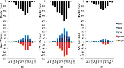
The average monthly flux values of water balance components in the annual average, wet year, and dry year are presented in Fig. 12. The surface water systems (i.e. the water yield of the watershed) consist of the surface runoff to streams (surq), lateral flow to streams (latq), and groundwater flow to streams (gwq, i.e. groundwater discharge), while the groundwater system is a combination of the water percolation to groundwater (perco) and seepage from rivers to the aquifer (swgw, i.e. river seepage). As a simulated result, the largest portion of surface water recharge is attributed to a lateral flow, followed by surface runoff and groundwater flow. The main component of groundwater recharge is the water percolated from the ground surface. The average annual recharge of surface water and groundwater (Fig. 12(a)) is about 290 mm and 325 mm, respectively, accounting in total for half of the annual rainfall (1120 mm). The surface water section can be separately recharged by 110, 155, and 25 mm of the surface runoff, lateral flow, and groundwater flow to stream, respectively. Meanwhile, the groundwater recharge section is summed from 315 mm of water percolation and 10 mm of river seepage.

In the wet year (Fig. 12(b)), due to a 500 mm increase in precipitation during May–October (the wet season), the surface runoff, lateral flow, and groundwater flow to streams increased by 170, 90, and 25 mm, respectively, while the water percolation and river seepage to the aquifer increased by 305 and 15 mm, respectively. Surface runoff and groundwater discharge contribute to flooding proportionally to their average annual values, with surface runoff providing most of the increase in river discharge. Therefore, an approximate doubling in the volume of groundwater discharging to streams and a 2.5 times increase in surface water runoff affected the occurrence of the great flood event that year.

In the dry year (Fig. 12(c)), recharges from surface runoff, lateral flow, and groundwater flow to streams are below average at 85, 70, and 15 mm, respectively, in the wet season because of decreased precipitation (400 mm). The groundwater recharges (perco and swgw) are reduced by 225 mm, accounting for almost 75% of the average annual condition. These cause a significant decrease in groundwater storage volume, which is the main water supply in this area, thus followed by severe drought events that year. Most importantly, the deficit in surface runoff and groundwater discharge occurs at the beginning of the wet season (May and July), which probably leads to insufficient water supply for both irrigation and domestic water use during the agricultural growing season.

Implications for water management

In conjunctive water-use management, groundwater head plays an important role, indicating the direction of groundwater flow. Changes in groundwater head indicate changes in the available water volume within an aquifer and provide a relative measure of its capacity to uptake or release water. High groundwater heads suggest a limited capacity for storing more water from rainfall and higher risk of fluvial or groundwater flooding. The river will be fed by the groundwater when the groundwater head is higher than the river stage, which can be followed by flood events if the drainage capacity is exceeded, whereas low groundwater head means that there is less water stored in the aquifer. If the groundwater head is lower than the river stage, the water contained in the river will recharge into the aquifer, which can be followed by drought events in years with low rainfall. Therefore, understanding changes in groundwater head under scenarios for different weather years can provide valuable information for mitigating flood and drought disasters effectively.

The spatially varied recharge, interaction with streams, and groundwater pumping results in a change of groundwater head are shown in Fig. 13. On average annuallly during 2007–2016 (Fig. 13(a)), the groundwater head in 80% of the watershed area is increased, where several plains areas are higher than 1 m, while some areas downstream have an increment of groundwater head of less than 1 m. The areas experiencing a decrease in groundwater head are mainly in high terrain, particularly the high mountains in the Nan River basin. In the wet year (Fig. 13(b)), the areas with an increased groundwater head are enlarged by 10% due to an increase in groundwater recharge. About 54% of the area has an increment of groundwater head exceeding 1 m. Nonetheless, the groundwater head in the mountain areas remains diminished. In the dry year (Fig. 13(c)), the areas with a low groundwater head are expanded by 8%, particularly in the downstream areas. The areas that contain an increase in the groundwater head of more than 1 m seem to be reduced by 14%.

Figure 13. Changes in groundwater (GW) head in the Yom and Nan river basins: (a) average annual (2007–2016); (b) during the wet year (2011); and (c) during the dry year (2015)

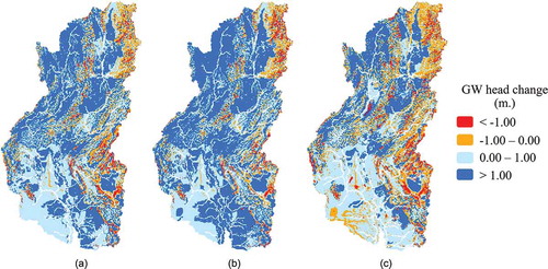
According to the average annual groundwater recharge, surface water–groundwater interactions, and spatial distribution of groundwater pumping (Fig. 14), the downstream area of the watershed is vulnerable to floods and droughts. This is evident because most of them are in the plains area, providing high increased groundwater head during the wet year and also dramatically decreased groundwater head during the dry year. The lower Yom River basin has often suffered from flood and drought events because of a low groundwater recharge rate, lack of a dam, high river seepage, and large groundwater pumping volume, which affect the potential for water storage. In addition, these factors also cause a high risk of flooding in years with heavy rainfall, and result in more drought in dry years.

Figure 14. Spatial distribution of average annual (a) groundwater recharge and (b) groundwater discharge to river; and (c) daily groundwater pumping in the Yom and Nan river basins

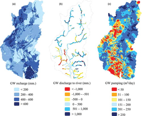
The approach presented in this study, for a sustainable solution to flood and drought, is to capture the surface runoff and potential recharge volumes during the wet season by recharging to the aquifer to reduce the intensity of flooding and also to supply in the dry season or coming droughts. Pavelic et al. (2012) proposed that dedicating 200 km² land area for recharging surplus water volumes from the downstream of this area to the shallow alluvial aquifers could mitigate the magnitude of flooding and socio-economic impacts without significant effects on ecosystems or on the large and medium storage. Considering this, the area with the potential to be used as groundwater banking is the middle plains areas of the basin, due to its high groundwater recharge rates and large number of pumping wells, which can reduce costs of storage and pumping for water supply.

The severity of flood and drought in the downstream area seems to be lower for the Nan River basin than the Yom River basin because of a large recharge volume from groundwater into river branches; additionally, the water upstream can be managed by the Sirikit Dam to reduce the magnitude of flooding and to store against water shortage. Meanwhile, a high groundwater recharge rate in this area contributes to water percolation and capture in the aquifer, whereas, according to low groundwater heads in the average year, wet year, and dry year, high terrain or mountain areas especially in the upstream are vulnerable to drought events. A low recharge of groundwater in these areas can cause difficulty in water storage and high irrigation costs. Even when there is a high groundwater discharge to the river and low amounts of groundwater pumping in plains areas, which can cause a large volume of groundwater storage, it is insufficient to meet water demand, particularly for agriculture. The application of a retention pond or groundwater banking is limited by the area available, while implementation in high-terrain areas requires a large budget. Therefore, the optimum approach should be increasing the river capacity and forest area to provide more water storage and to retard the flow of water at the same time.

Summary and conclusions

This study presented the SWAT-MODFLOW model for integrating surface water–groundwater flow in the Yom River and Nan River basins of Thailand and demonstrated the model’s excellent performance. The integration between SWAT and MODFLOW models was implemented using the QGIS plug-in tool QSWATMOD interface, with spatially varied aquifer properties such as hydraulic conductivity, specific yield, and specific storage for MODFLOW. The model also accounted for groundwater pumping that has occurred in the river basins since 2009. According to graphical-statistical comparisons of measured and simulated river discharge and groundwater heads, the simulation results replicated the observation data in both magnitude and pattern. Groundwater pumping was shown to be a significant component of the groundwater flow system and must be included to match the observed groundwater levels.

In the wet year (2011), the surface water recharge and groundwater were about twice higher than the average annual value. Areas with an increase in the groundwater head were enlarged by 10%. Consequently, half of the watershed area contained an increase in the groundwater head greater than 1 m. In the dry year (2015), recharges of surface water and groundwater were 3 times below the average. Areas with a decrease in the groundwater head were expanded by 8%, particularly the downstream. Meanwhile, the area exceeding 1 m in increased groundwater head was reduced by 14%.

The majority interaction in main streams was groundwater discharge to the river, especially the upstream area, while river seepage to the aquifer was mostly detected in the river branches and downstream area, due to low groundwater levels. The groundwater discharged to the river was over 500 mm in several parts of the rivers in the wet year. Sections that displayed river seepage to the aquifer of less than 500 mm became areas of groundwater discharge to the river. The streams with river seepage higher than 500 mm stayed the same as the average annual value. In the dry year, the ratio of streams with recharge from the groundwater higher than 500 mm was reduced to 2 times below the average, especially in the Yom River basin. River seepage sections higher than 500 mm were decreased one-three.

Results from this study enhance our understanding of surface water–groundwater regimes and their interactions in the Yom River and Nan River basins. Due to model accuracy in both stream discharge and groundwater head simulation, the calibrated SWAT-MODFLOW model can be used as a decision support tool in water management planning for the coming decades. Capturing surplus water volumes during the wet season, using aquifer recharge management, to shallow alluvial aquifers in the middle plains areas could be a sustainable solution for flood and drought issues in the Yom River basin. For the Nan River basin, in contrast, the appropriate approach is to improve the stream’s capacity in terms of forest areas to increase the water storage and retard the flow of water.

Acknowledgements

This research was supported by King Mongkut’s University of Technology Thonburi’s Post-doctoral Fellowship. The authors also thank the Department of Civil and Environmental Engineering, Colorado State University, for hosting Mr Petpongpan during the research project.

Disclosure statement

No potential conflict of interest was reported by the authors.

Additional information

Funding

This work was supported by the King Mongkut’s University of Technology Thonburi [Post-doctoral Fellowship].

References

- Achieng, D.O., et al., 2015. Conjunctive use of surface and groundwater as agri-tourism resource facilitator: discourse analysis for planning in developing nations. IOSR Journal of Computer Engineering, 17 (1), 77–86.
- Aliyari, F., et al., 2019. Coupled SWAT-MODFLOW model for large-scale mixed agro-urban river basins. Environmental Modelling & Software, 115, 200–210. doi:https://doi.org/10.1016/j.envsoft.2019.02.014
- Apipattanavis, S., Ketpratoom, S., and Kladkempetch, P., 2018. Water management in Thailand. Irrigation and Drainage, 67 (1), 113–117. doi:https://doi.org/10.1002/ird.2207
- Arnold, J.G., et al., 2012. Soil & water assessment tool-input/output documentation; Version 2012 [online]. College Station: Texas Water Resources Institute. Available from: https://swat.tamu.edu/docs/ [Accessed 4 May 2020].
- Arnold, J.G., et al., 1998. Large area hydrologic modeler and assessment part I: model development. Journal of the American Water Resources Association, 34, 73–89. doi:https://doi.org/10.1111/j.1752-1688.1998.tb05961.x
- Bailey, R., et al., 2017. SWATMOD-Prep: graphical user interface for preparing coupled SWAT-MODFLOW simulations. Journal of the American Water Resources Association, 53 (2), 400–410. doi:https://doi.org/10.1111/1752-1688.12502
- Bailey, R.T., et al., 2016. Assessing regional-scale spatio-temporal patterns of groundwater–surface water interactions using a coupled SWATMODFLOW model. Hydrological Processes, 30 (23), 4420–4433.
- Bejranonda, W., Koch, M., and Koontanakulvong, S., 2011. Surface water and groundwater dynamic interaction models as guiding tools for optimal conjunctive water use policies in the central plain of Thailand. Environmental Earth Sciences, 70, 2079–2086. doi:https://doi.org/10.1007/s12665-011-1007-y
- Bejranonda, W., Koontanakulvong, S., and Koch, M., 2007. Surface and groundwater dynamic interactions in the Upper Great Chao Phraya Plain of Thailand : semi-coupling of SWAT and MODFLOW. In: IAH-2007 Groundwater and Ecosystems, 17–21 September 2007. Lisbon, Portugal.
- Cho, J., Mostaghimi, S., and Kang, M.S., 2010. Development and application of a modeling approach for surface water and groundwater interaction. Agricultural Water Management, 97 (1), 123–130. doi:https://doi.org/10.1016/j.agwat.2009.08.018
- Chu, M.L., et al., 2013. Impacts of urbanization on river flow frequency: a controlled experimental modeling-based evaluation approach. Journal of Hydrology, 495, 1–12. doi:https://doi.org/10.1016/j.jhydrol.2013.04.051
- Chunn, D., et al., 2019. Application of an integrated SWAT-MODFLOW model to evaluate potential impacts of climate change and water withdrawals on groundwater–surface water interactions in west-central Alberta. Water (Switzerland), 11 (1), 110.
- Dowlatabadi, S. and Zomorodian, S.M., 2015. Conjunctive simulation of surface water and groundwater using SWAT and MODFLOW in Firoozabad watershed. KSCE Journal of Civil Engineering, 20 (1), 485–496. doi:https://doi.org/10.1007/s12205-015-0354-8
- Gao, F., et al., 2019. Assessment of surface water resources in the Big Sunflower River Watershed using coupled SWAT-MODFLOW model. Water, 11 (3), 528. doi:https://doi.org/10.3390/w11030528
- Guzman, J.A., et al., 2015. A model integration framework for linking SWAT and MODFLOW. Environmental Modelling and Software, 73 (April 2016), 103–116. doi:https://doi.org/10.1016/j.envsoft.2015.08.011
- Hu, L., Xu, Z., and Huang, W., 2016. Development of a river-groundwater interaction model and its application to a catchment in Northwestern China. Journal of Hydrology, 543, 483–500. doi:https://doi.org/10.1016/j.jhydrol.2016.10.028
- Hydro and Agro Informatics Institute, 2012. Information of 25 main basins in Thailand [online]. Hydro and Agro Informatics Institute. Available from: http://www.thaiwater.net/web/index.php/knowledge/128-hydro-and-weather/663-25basinreports.html [Accessed 4 May 2020].
- Joo, J., et al., 2018. An integrated modeling approach to study the surface water–groundwater interactions and influence of temporal damping effects on the hydrological cycle in the Miho catchment in South Korea. Water (Switzerland), 10 (11), 1529.
- Kim, N.W., et al., 2008. Development and application of the integrated SWAT-MODFLOW model. Journal of Hydrology, 356 (1–2), 1–16. doi:https://doi.org/10.1016/j.jhydrol.2008.02.024
- Kollet, S., et al., 2016. The integrated hydrologic model intercomparison project: a second set of benchmark results to diagnose integrated hydrology and feedbacks. Water Resources Research, 53, 867–890. doi:https://doi.org/10.1002/2016WR019191
- Li, R., et al., 2016. Evaluating hydrologically connected surface water and groundwater using a groundwater model. Journal of the American Water Resources Association, 52 (3), 799–805. doi:https://doi.org/10.1111/1752-1688.12420
- Malcolm, I.A., et al., 2003. Heterogeneity in ground water–surface water interactions in the hyporheic zone of a salmonid spawning stream. Hydrological Processes, 17 (3), 601–617. doi:https://doi.org/10.1002/hyp.1156
- Molina-Navarro, E., et al., 2019. Comparison of abstraction scenarios simulated by SWAT and SWAT-MODFLOW. Hydrological Sciences Journal, 64, 434–454. doi:https://doi.org/10.1080/02626667.2019.1590583
- Moriasi, D.N., et al., 2007. Model evaluation guidelines for systematic quantification of accuracy in watershed simulations. Transactions of the American Society of Agricultural and Biological Engineers, 50 (3), 885–900.
- Nash, J.E. and Sutcliffe, J.V., 1970. River flow forecasting through conceptual models part I - A discussion of principles. Journal of Hydrology, 10, 282–290. doi:https://doi.org/10.1016/0022-1694(70)90255-6
- Neitsch, S.L., et al., 2011. Soil and Water Assessment Tool Theoretical Documentation Version 2009 [online]. Grassland: Soil and Water Research Laboratory, Agricultural Research Service. Available from: https://swat.tamu.edu/media/99192/swat2009-theory.pdf [Accessed 4 May 2020].
- Park, S. and Bailey, R.T., 2017. SWAT-MODFLOW Tutorial: documentation for preparing model simulations [online]. Department of Civil and Environmental Engineering, Colorado State University. Available from: https://swat.tamu.edu/media/115048/swat-modflow-tutorial.pdf [Accessed 4 May 2020].
- Park, S., et al., 2019. A QGIS-based graphical user interface for application and evaluation of SWAT-MODFLOW models. Environmental Modelling and Software, 111, 493–497. doi:https://doi.org/10.1016/j.envsoft.2018.10.017
- Pavelic, P., et al., 2012. Balancing-out floods and droughts: opportunities to utilize floodwater harvesting and groundwater storage for agricultural development in Thailand. Journal of Hydrology, 470–471, 55–64. doi:https://doi.org/10.1016/j.jhydrol.2012.08.007
- Petpongpan, C., Ekkawatpanit, C., and Kositgittiwong, D., 2020. Climate change impact on surface water and groundwater recharge in Northern Thailand. Water, 12 (4), 1029. doi:https://doi.org/10.3390/w12041029
- Petpongpan, C., et al., 2021. Projection of hydro-climatic extreme events under climate change in Yom and Nan River Basins, Thailand. Water, 13 (5), 665. doi:https://doi.org/10.3390/w13050665
- Playan, E. and Mateos, L., 2006. Modernization and optimization of irrigation systems to increase water productivity. Agricultural Water Management, 80, 100–116. doi:https://doi.org/10.1016/j.agwat.2005.07.007
- Semiromi, M.T. and Koch, M., 2019. Analysis of spatio-temporal variability of surface-groundwater interactions in the Gharehsoo river basin, Iran, using a coupled SWAT-MODFLOW model. Environmental Earth Sciences, 78, 201. doi:https://doi.org/10.1007/s12665-019-8206-3
- Sophocleous, M., 2002. Interactions between groundwater and surface water: the state of the science. Hydrogeology Journal, 10 (1), 52–67. doi:https://doi.org/10.1007/s10040-001-0170-8
- Sophocleous, M. and Perkins, S.P., 2000. Methodology and application of combined watershed and ground-water models in Kansas. Journal of Hydrology, 236 (3–4), 185–201. doi:https://doi.org/10.1016/S0022-1694(00)00293-6
- Sophocleous, M.A., et al., 1999. Integrated numerical modeling for basin-wide water management: the case of the Rattlesnake Creek basin in south-central Kansas. Journal of Hydrology, 214, 179–196. doi:https://doi.org/10.1016/S0022-1694(98)00289-3
- Sudicky, E.A., et al., 2008. Simulating complex flow and transport dynamics in an integrated surface-subsurface modeling framework. Geosciences Journal, 12, 107–122. doi:https://doi.org/10.1007/s12303-008-0013-x
- Wei, X. and Bailey, R.T., 2019. Assessment of system responses in intensively irrigated stream-aquifer systems using SWAT-MODFLOW. Water, 11 (8), 1576. doi:https://doi.org/10.3390/w11081576
- Winter, T.C., 1995. Recent advances in understanding the interaction of groundwater and surface water. Reviews of Geophysics, 33, 985–994. doi:https://doi.org/10.1029/95RG00115
- Wu, J., et al., 2018. Evaluating the interactions between surface water and groundwater in the arid mid-eastern Yanqi Basin, northwestern China. Hydrological Sciences Journal, 63 (9), 1313–1331. doi:https://doi.org/10.1080/02626667.2018.1500744