Assessing the potential and hydrological usefulness of the CHIRPS precipitation dataset over a complex topography in Pakistan

ABSTRACT

This study evaluates the spatial and temporal performance of the Climate Hazard Group InfraRed Precipitation Satellite (CHIRPS) against Tropical Rainfall Measuring Mission (TRMM) Multi-Satellite Precipitation Analysis (TMPA) 3B42/3B43 v. 7 and Global Precipitation Measurement (GPM)-based Integrated Multi-Satellite Retrievals for GPM (IMERG V06), from 2000 to 2013. Several statistical metrics were used to assess the performance of CHIRPS over the Indus Basin, and its hydrological utility is also assessed using the Soil and Water Assessment Tool (SWAT). The Gilgit and Soan basins were selected for hydrological modelling. The results demonstrate the spatial and temporal dependency of CHIRPS, i.e. better performance was observed in the Lower Indus Basin (LIB) while poor performance was observed in the Upper Indus Basin (UIB). The hydrological assessment of CHIRPS revealed poor performance (overestimation of streamflow) across the Gilgit Basin during both calibration and validation periods. Satisfactory to good performance was obtained across the Soan Basin.

KEYWORDS:

• satellite precipitation
• CHIRPS
• TMPA
• IMERG
• Indus Basin
• SWAT
• SWAT-CUP
• Gilgit Basin: Soan Basin
• Pakistan

Editor S. Archfield Associate editor D. Rivera

1 Introduction

Precipitation is an indispensable component of the hydrological cycle and plays a vital role in hydrological modelling (Ebert et al. 2007, Price et al. 2014, Rahman et al. 2020a). It also influences human-associated activities like agriculture and drinking (Gebere et al. 2015, Liu 2015). However, catastrophic natural disasters like droughts and floods are actuated by excessive precipitation (Gebere et al. 2015, Guo et al. 2016). Pakistan ranks as the sixth most populous country in the world and is extensively vulnerable to natural disasters due to climate change (Pakistan ranks seventh among the countries affected most severely by climate change; Eckstein et al. 2017, Shahid and Rahman 2020). During the last few decades, the frequency of occurrence of natural disasters has increased in Pakistan, and this has affected the country’s economy (Khan et al. 2014). The 2010 flood is a tragic moment in the country’s history, which drastically damaged agriculture and infrastructure and took thousands of lives (Rahman et al. 2019). Studies on flood and drought assessment demonstrated that these events will become more frequent in the country, an increase that is triggered by climate change (Khan et al. 2016, Hussain et al. 2018). Therefore, producing precise precipitation estimates is extremely important as it can significantly influence the process of mitigating the impacts of extreme events. Understanding the spatial and temporal variability of precipitation is a critical factor in comprehending the hydrological cycle, whereas precipitation trend analysis can be used for decision support.

Despite its importance, it is still a challenging task to estimate precise precipitation at high spatial and temporal resolutions (Chiaravalloti et al. 2018, Gao et al. 2018). Raingauges (RGs) and weather radar (WR) are the conventional sources used to measure/estimate precipitation at the local scale (Muhammad et al. 2018). However, RGs and WR are sparsely distributed, which makes it arduous to capture the spatio-temporal variability in precipitation, especially in mountainous regions (Steiner et al. 2003, Yong et al. 2012, Mei et al. 2016, Ma et al. 2018). However, advances in remote sensing offer satellite-based precipitation datasets (SPDs) of various spatial and temporal resolutions with long-term records. The SPDs are complementary to RGs and WR and provide continuous monitoring of precipitation over regional and global scales. Moreover, SPDs overcome the data scarcity problems that occur when RGs are sparsely distributed or when areas are ungauged (Rahman et al. 2020b). However, there are no best-performing SPDs that produce superior results worldwide; therefore, SPDs must be evaluated before any application for each study area. SPDs such as Tropical Rainfall Measuring Mission (TRMM) Multi-Satellite Precipitation Analysis (TMPA), Precipitation Estimation from Remotely Sensed Information using Artificial Neural Networks (PERSIANN), Climate Prediction Center MORPHing (CMORPH), Global Precipitation Measurement (GPM)-based Integrated Multi-Satellite Retrievals for GPM (IMERG) and several others provide precipitation estimates with a high spatial resolution.

The long-term precipitation record is indispensable for understanding the hydrological response and for better management of water resources, especially in regions with sparse meteorological observatories (Yao et al. 2016, Yang et al. 2017; Duan et al. 2019). SPDs are favoured for developing countries like Pakistan that are characterized by the scant distribution of RGs and by poorly gauged/ungauged watersheds, due to the free availability of SPD data over large spatial and temporal domains. A wide range of studies have evaluated the suitability of SPDs on global and regional scales by comparing the precipitation records from SPDs with precipitation records from RGs using both pixel-by-pixel and point-to-pixel analyses (Khan et al. 2014, Prakash et al. 2014, Shukla et al. 2014), for Asia (Dinku et al. 2007, Pierre et al. 2011, Thiemig et al. 2012), Africa (Vila et al. 2009, Ochoa-Sánchez et al. 2014, Satgé et al. 2016), and South America and Europe (Kidd et al. 2012). These studies reported that the performance of all SPDs varies from region to region, which may be due to differences in altitude, topographic complexity and climate as well as temporal dependency, seasonality and precipitation intensity (Dinku et al. 2010, Rahman et al. 2018, 2020c). Generally, the performance of TMPA is considered better for moderate rainfall events at sub-continent scale (Nair et al. 2009, Hussain et al. 2018), CMORPH performs well in the mountainous region of East Africa (Dinku et al. 2007, 2010), and PERSIANN has high accuracy across plains and dry regions (Gebere et al. 2015, Satgé et al. 2016) over Eastern Ethiopia.

Very few studies have assessed the performance of SPDs across the Indus Basin of Pakistan (Cheema and Bastiaanssen 2012, Khan et al. 2014, Anjum et al. 2016, Hussain et al. 2018, Iqbal and Athar 2018, Rahman et al. 2018, 2019, Ullah et al. 2019, Satgé et al. 2021). Cheema and Bastiaanssen (2012) evaluated the performance of TRMM over Pakistan at a monthly time scale. They concluded that TRMM overestimated the precipitation at high elevations while it underestimated the precipitation in coastal areas. Khan et al. (2014) performed a seasonal (monsoon) assessment of CMORPH and TMPA at a daily time scale and reported better performance of TMPA. Anjum et al. (2016) evaluated TMPA V06 and V07 across Swat catchment (a sub-basin of Indus Basin), and concluded that both products are suitable at the monthly scale. Hussain et al. (2018) evaluated TMPA, CMORPH and PERSIANN SPDs over different climatic regions of Pakistan. They found that all products performed well in mountain regions compared to plains regions. Moreover, these products overestimated precipitation in glacial regions. Rahman et al. (2018) evaluated the performance of TMPA, IMERG, PERSIANN-Climate Data Record and PERSIANN SPDs over Pakistan. They concluded that IMERG and TMPA performed well.

The Climate Hazards Group Infrared Precipitation Satellite (CHIRPS) is a newly developed climatic database or precipitation dataset (Funk et al. 2014). Three types of information are merged to develop the CHIRPS: satellite estimates, global climatology and in situ data. CHIRPS provides precipitation records from 1981 to the present with a very high spatial resolution of 0.05°. The CHIRPS SPD is evaluated in different parts of the world, including Cyprus (Paredes-Trejo et al. 2017), Brazil (Katsanos et al. 2016), Nepal (Mainali and Pricope 2017), Italy (Tuo et al. 2016), Mozambique (Toté et al. 2015), Vietnam (Guo et al. 2017) and China (Bai et al. 2018). Studies show that CHIRPS performs well when compared with RG observations. However, the reliability of CHIRPS has not been extensively assessed over the topographically complex and climatically diversified Indus Basin of Pakistan.

Therefore, the objectives of the current study are to comprehensively evaluate CHIRPS at various spatial and temporal scales over the Indus Basin in Pakistan and to compare its performance with other SPDs that were previously extensively evaluated (TMPA 3B42/3B43 v. 7 and IMERG V06), during 2000–2013. The Indus Basin of Pakistan is divided into three distinct climate basins: the Upper Indus Basin (UIB), Middle Indus Basin (MIB), and Lower Indus Basin (LIB). Moreover, the Soil and Water Assessment Tool (SWAT) is employed to test the hydrological utility of the CHIRPS dataset across UIB (Gilgit Basin) and MIB (Soan Basin), and compared with ground-based flow gauge records and RG-simulated streamflow. In the present study, a network of 59 RGs across the Indus Basin in Pakistan is used to evaluate the performance of CHIRPS during 2000–2013.

2 Study area

2.1 Study area for spatial and temporal evaluation of SPDs

The Tibetan Plateau is the source for the Indus Basin; it spreads over the Hindu Kush Himalayas (HKH) region and has an area of 1 120 000 km². In the present study, the study area comprises the major parts of the Indus Basin (i.e. UIB, MIB, and LIB), situated in Pakistan. The study area (Fig. 1(a)) is situated at latitude 24.02–37.07°N and longitude 66.2–82.5°E and covers an area of 855 045 km². The Indus Basin has a diverse topography, where more than 40% of the basin has an elevation of more than 4000 metres above mean sea level (a.m.s.l.). Tributaries of the Indus River, such as Jhelum, Ravi, Sutlej and Chenab rivers, flow through the Indus Basin where it enters Pakistan and are the major sources of water supply for agricultural, industrial and domestic needs (Kalair et al. 2019).

Figure 1. (a) Geographical location of Indus Basin, Gilgit Basin and Soan Basin; (b) elevation map of Gilgit Basin; (c) elevation map of Soan Basin

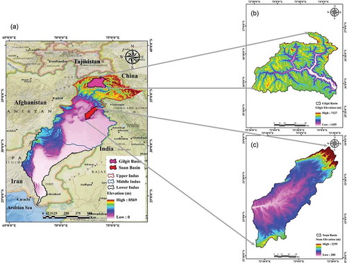
The Indus Basin is considered one of the most important basins of the world in terms of human dependency (Laghari et al. 2012). The livelihood of 215 million people is directly or indirectly dependent on the Indus River. The population density in the Indus Basin is very high, where the approximate availability of water per head per annum is 1329 m³. The Indus River is the main tributary of the Indus Basin supplying water for the downstream area of the basin. This basin also contains one of the largest integrated irrigation systems of the world (Pathak 2012).

In the current study, the Indus Basin is divided into three parts (Liviu Giosan et al. 2006), and the performance of SPDs is evaluated in each part of the basin. UIB consists of the glacial area and parts of the humid region comprising the high mountains of the Hindukush Himalayas, and is the origin of all the major rivers of Pakistan. The severe glacier melt across UIB in the summer season can cause flooding in the downstream area. The MIB comprises lower areas of humid and arid regions, mostly the plains of Punjab province. The capital of Pakistan, Islamabad, lies in the MIB, and gets its drinking water supply from the Soan River, a tributary of the Indus Basin (Shahid et al. 2018, 2020). The agriculture in MIB is entirely dependent on precipitation and the integrated irrigation network. The LIB includes the extremely arid regions of South Punjab and Sindh provinces of Pakistan. The principal tributaries of the Indus River meet there at the city of Bahawalpur; and, finally, the Indus River drains into the Arabian Sea.

The precipitation trend across the Indus Basin is minimum precipitation (<100 mm/month) in UIB (34–36°N), high precipitation (>700/month) downstream of UIB and upstream of MIB (extreme northeast) between 29 and 33°N, and again low (around 100/month) downstream of MIB and in the entire LIB between 24 and 28°N (Iqbal and Athar 2018, Rahman et al. 2018). Overall, precipitation in Indus Basin varies spatially from 1500 mm/a (in the high-elevation regions of the north) to 100 mm/a (in the low-elevation regions of the south). Winter and monsoon are the dominant precipitation seasons, where western disturbances cause intense to moderate precipitation (Dimri et al. 2015). During the monsoon season, Pakistan receives around 55% to 60% of its annual precipitation, while 30% occurs during the winter season (Asmat and Athar 2017).

2.2 Study areas for the hydrological evaluation of CHIRPS

Gilgit Basin (Fig. 1(b)) is one of the poorly gauged basins of the UIB, with few climate stations. The stations within or in the vicinity of Gilgit Basin are Gupis, Yasin, Ushkore and Gilgit. The mean monthly calculated minimum and maximum temperature ranges are from −2.2 to 18.5°C and 9.2 to 36.5°C, respectively. The mean annual precipitation observed in Gilgit Basin is 175.4 mm, while the mean annual streamflow observed at Gilgit gauge station is 275.3 m³/s. The collected meteorological/climate and streamflow data are used as a direct input to SWAT without interpolation, as the available stations do not meet the requirements for the interpolation method. Figure 2(a and b) depicts the land-use and soil maps for Gilgit Basin used in the calibration and validation of SWAT. The land-use map was developed using the supervised classification method by employing imagery from LANDSAT VII Enhanced Thematic Mapper Plus using the support vector machine (SVM) method (Balkhair and Ur Rahman 2019). Supervised classification segments the spatial-spectral domain into regions related to ground-based land-use classes. The land-use map of Gilgit Basin is divided into six classes, i.e. forest, agriculture, barren land, lakes, water bodies and residential areas. The global soil map, developed by the Food and Agriculture Organization of the United Nations (FAO) at a 1:5 000 000 spatial resolution, is employed to extract the soil layers for the Gilgit Basin (http://www.fao.org/soils-portal/soil-survey/soil-maps-and-databases/faounesco-soil-map-of-the-world/en/). The land-use and soil maps were generated for the year 2005, which is the median year of flow simulation, i.e. SWAT analysis is carried out during 2000–2010. The climate data, including precipitation, relative humidity, temperature, wind speed and solar radiation of Gilgit and Gupis RGs, were used for streamflow simulation in ArcSWAT 2012. The Gilgit flow gauge data were used for the calibration and validation of the SWAT model in Gilgit Basin.

Figure 2. (a) Land-use map of Gilgit Basin; (b) soil map extracted from the Food and Agriculture Organization global soil map for Gilgit Basin; (c) land-use map of Soan Basin; (d) soil map extracted from the Food and Agriculture Organization global soil map for Soan Basin

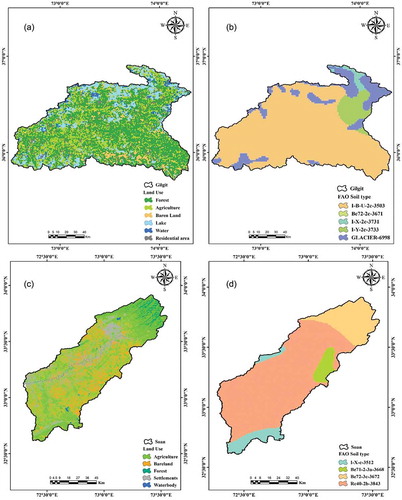
Figure 1(c) shows the geographical location of Soan Basin in the MIB; it has a catchment area of 6842 km² and its elevation ranges from 280 to 2255 m with a gentle to steep slope. The Soan River is a main river of the Soan Basin, which originates from Murree and is considered the hydrological unit of Potohar plateau, Pakistan. Monsoon precipitation-fed streams are a major source of flow for the Soan Basin. The mean annual precipitation of Soan Basin was 1465 mm during the period 1983–2012 (Shahid et al. 2018). The Soan River supplies water to the Simly Dam, which provides drinking water to Islamabad and Rawalpindi. The Soan River fulfills the irrigation requirements of the Potohar plateau, and during the last decade, various projects have been carried out to improve the irrigation (Shahid et al. 2018). Figure 2(b and c) presents land use (developed using SVM method) and soil (extracted from FAO global soil map) maps for Gilgit and Soan basins.

Climate data including precipitation, solar radiation, temperature, wind speed and relative humidity from four stations (i.e. Murree, Islamabad, Kalandar and Chakwal) were used as input for flow simulation across Soan Basin in ArcSWAT 2012. The SWAT model was calibrated and validated at two flow gauges, namely Chirah (upstream) and Sill River station (downstream). In contrast, Gupis and Gilgit stations were used as input stations for climate data while SWAT was calibrated and validated at Gilgit station.

3 Datasets

3.1 Description of RG data

The Pakistan Meteorological Department (PMD) and Water and Power Development Authority (WAPDA) under the Snow and Ice Hydrology Project (SIHP) mainly collect the RG precipitation records for the Indus Basin in Pakistan. RGs located at high elevations, which are mostly found in UIB, are operated under SIHP. Precipitation data at a daily temporal scale over 65 RGs were collected from both organizations, of which the data from 59 RGs were used for the current study (shown in Fig. 1(a)). The temporal span for the collected data ranges from 2000 to 2013. Of the 59 RGs, the precipitation data for 45 RGs were obtained from PMD while WAPDA provided the data for 14 RGs. The meteorological stations in UIB are named RU1 to RU31; MIB is denoted by RM1 to RM16; and LIB stations are named RL1 to RL12. PMD and WAPDA collect the precipitation records manually, which might be exposed to a number of instrumental and human errors. The stations sited in UIB (high elevations) may also have errors caused by wind, which can affect the data quality. In this context, the observed data were rectified by PMD and WAPDA following the World Meteorological Organization (WMO) standard code (WMO-N). Moreover, to assure high-quality data, skewness and kurtosis methods were performed to evaluate the quality of the collected precipitation records, while the zero-order method was used to fill in the missing data found in a few RGs, following Rahman et al. (2018). The RGs data of both organizations were used as reference data to evaluate the performance of the selected SPDs.

3.2 Description of satellite-precipitation datasets

The daily data of CHIRPS v. 2 (hereinafter CHIRPS) were downloaded from the website of the University of California, Santa Barbara (USA). It is a blended precipitation product, which combines pentad precipitation data. The CHIRPS data are developed in different stages. The primary data sources used for CHIRPS include geostationary observations from the Climate Prediction Center (CPC), Climate Hazards Group’s Precipitation Climatology (CHPClim), National Oceanic and Atmospheric Administration (NOAA), TRMM estimated data and in situ (RG) precipitation data obtained from national and regional meteorological stations (Funk et al. 2014). The spatial resolution of CHIRPS is approximately 5.3 km (0.05°), and its coverage is between 50°S and 50°N, and between 180°E and 180°W (Funk et al. 2014, Bai et al. 2018). Detailed information on CHIRPS estimates is given in the references (Bai et al. 2018, Nogueira et al. 2018, Saeidizand et al. 2018).

The CHIRPS dataset processing stream incorporates data from five public and a number of private data streams. The public data streams include the Global Historical Climatology Network (GHCN) at daily and monthly time scales, Global Telecommunication System (GTS), Global Summary of the Day (GSOD) and Southern African Science Service Centre for Climate Change and Adaptive Land Management (SASSCAL) (www.sasscalweathernet.org). In the current study, overall 65 stations were obtained from PMD and WAPDA, of which six stations were discarded to avoid biasing the results. Moreover, a very limited number of RGs were used to generate precipitation data from CHIRPS over Pakistan (Nawaz et al. 2021).

CHIRPS was evaluated with TMPA 3B42 v. 7 and 3B43 v. 7, and with IMERG. TRMM, launched in November 1997, was jointly developed by the Japan Aerospace Exploration Agency (JAXA) and the US National Aeronautics and Space Administration (NASA). Three instruments are used to record the precipitation in TRMM: TRMM microwave (MW) image, precipitation radar (PR) and visible infrared scanner (VIS). The TMPA has been widely used in the past few decades, and it has two types of products: 3B42 v. 6 and 3B42 v. 7. These products are gauge adjusted and provide the data from 50°S to 50°N. The TMPA algorithm uses estimates from various satellites and gauges to generate best precipitation estimates (Simpson et al. 1988, Kummerow et al. 1998, 2000). During the past decade, three significant improvements have been made in the TMPA algorithm, and new satellite sensors have been added. A detailed description and recent changes of TRMM (TMPA) are discussed by Huffman et al. (2015). The daily and monthly precipitation products TMPA-3B42 v. 7 and 3B43 v. 7 are used in this study.

The CHIRPS performance is also compared with IMERG V06 on daily and monthly temporal scales (Huffman et al. 2018). IMERG was developed by NASA, which uses passive microwave (PMW) and infrared (IR) sensors from geostationary satellites and low Earth orbit (LEO). The whole process of precipitation estimation includes the application of the Goddard profiling algorithm (GPROF) to retreive precipitation from PMW datasets, which are calibrated to the GPM Combined Radar–Radiometer Algorithm (CORRA) derived from GPM MW imager (GMI) and dual-frequency precipitation radar (DPR). It also used monthly precipitation records of the Global Precipitation Climatology Centre (GPCP). Afterwards, PMW precipitation records were merged with PERSIANN-Cloud Classification System using the CMORPH-Kalman Filter (CMORPH-KF) Langrangian time interpolation. The blending process of IMERG relies on motion vectors retrieved from the top cloud temperature of CPC-IR to produce precipitation data at 30-min intervals (Huffman et al. 2018). IMERG is run 2 times to develop IMERG Early, Late and Final precipitation products at 4 h, 12 h, and 2.5 months, respectively. In the current study, we used the final run of IMERG V06 (hereinafter IMERG) for the performance comparison against CHIRPS.

3.3 Pre-processing of SPDs and RGs

The selected SPDs differ in spatial resolutions, i.e. spatial resolutions for CHIRPS, TMPA and IMERG are 0.05°, 0.25° and 0.10°, respectively. The spatial resolution of CHIRPS and IMERG is adjusted to the spatial resolution of TMPA (Yuan et al. 2017, Rahman et al. 2018). To avoid a mismatch issue, a coordinate-matching process is also performed. In this process, the latitude/longitude and precipitation records of the selected SPDs were compared with the satellite precipitation at each individual pixel. The mean precipitation is taken from pixels containing more than one RG in a single pixel; this can produce a single mean value for each pixel. The daily accumulation of SPDs was computed from 3:00 to 3:00 UTC to match the 8:00 to 8:00 Pakistan standard time (PST), which was the actual time for the RG data collection.

3.4 Performance evaluation of SPDs

Four continuous metrics, i.e. mean error (ME), root mean square error (RMSE), Pearson correlation coefficient (CC), and Kling-Gupta efficiency (KGE) score, are considered for the evaluation of CHIRPS and other SPDs at daily, monthly and annual time scales from 2000 to 2013. These metrics compare the precipitation records from SPDs with observed precipitation from RGs using point-by-pixel analysis. ME is a measure that describes the difference between SPD and RG precipitation estimates. CC is an index that represents the degree of agreement between SPDs and RGs. RMSE represents the average magnitude of the deviation/error (Xu et al. 2017). KGE score is the combination of several statistical metrics, including CC, variability ratio (γ) and bias ratio (β) (Gupta et al. 2009, Kling et al. 2012). KGE score is employed to assess the overall performance of CHIRPS SPD. “CC” in the KGE score computes the temporal variations in CHIRPS, while β and γ measure the precipitation volume and distribution, respectively. Overall, the lower the values of ME and RMSE, the better the performance of CHIRPS; and the higher the values of CC, the better the performance of CHIRPS. Further, the KGE score ranges from −∞ to 1, with 1 being the optimal value.

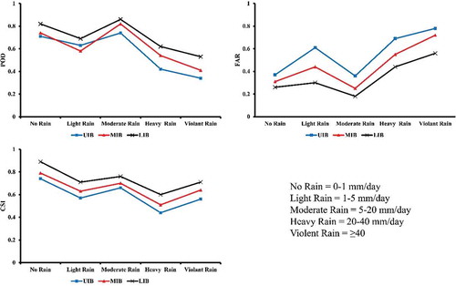
A set of categorical statistics is also adapted to appraise the ability of CHIRPS at different precipitation intensities. These statistics include the probability of detection (POD), false alarm ratio (FAR) and critical success index (CSI). POD assesses the potential of SPDs to correctly detect the rainfall events across all RGs. FAR represents the false detected rainfall events of the SPDs, whereas CSI indicates the overall fraction of rain events detected correctly by SPDs. Detailed descriptions and equations for these metrics are presented in Table 1. These categorical metrics were evaluated at different rainfall intensities following Zambrano-Bigiarini et al. (2017). The rainfall events (intensities) considered in the current study are no rain (0–1 mm/d), light rain (1–5 mm/d), moderate rain (5–20 mm/d), heavy rain (20–40 mm/d) and violent rain (≥40 mm/d).

Table 1. List of statistical metrics used to evaluate the performance of selected SPDs

Statistical index	Unit	Equation	Perfect value	Equation number
Mean error (ME)	mm	$\frac{1}{n}{\sum }_{i=1}^n(S_i-G_i)$	0	1
Root mean square error (RMSE)	mm	$RMSE=\sqrt{\frac{1}{n}\sum _{i=1}^n{\left(S_i-G_i\right)}^2}$	0	2
Correlation coefficient (CC)	NA	$CC=\frac{{\sum }_{i=1}^n\left(S_i-\bar{S}\right)\left(G_i-\bar{G}\right)}{\sqrt{{\sum }_{i=1}^n{\left(S_i-\bar{S}\right)}^2}\sqrt{{\sum }_{i=1}^n{\left(S_i-\bar{S}\right)}^2}}$$\mathrm{K}\mathrm{G}\mathrm{E}=1-\sqrt{{(R-1)}^2+{(\beta -1)}^2+{(\gamma -1)}^2}$	1	3
Kling-Gupta efficiency score (KGE)	NA	Where $\beta =\frac{\bar{E}}{M};\gamma =\frac{{\left(CV\right)}_E}{{\left(CV\right)}_M}$${\left(CV\right)}_E=\sqrt{\frac{1}{N}{\sum }_{i=1}^N\frac{\left(E_i-\bar{E}\right)}{\bar{E}}}$${\left(CV\right)}_M=\sqrt{\frac{1}{N}{\sum }_{i=1}^N\frac{\left(E_i-\bar{E}\right)}{\bar{E}}}$	1	4
Probability of detection (POD)	NA	$POD=\frac{a}{a+c}$	1	5
False alarm ratio (FAR)	NA	$FAR=\frac{b}{a+b}$	0	6
Critical success index (CSI)	NA	$CSI=\frac{a}{a+b+c}$	1	7

S_i and G_i shows the precipitation acquired from SPDs and RGs for the ith time step, where n represents sample size, and $\bar{S}$ and $\bar{G}$ represent the mean precipitation from SPDs and RGs, respectively. The term a represents the number of hits, b represents the number of false alarms and c represents the number of misses. Hits are events when both SPDs and RGs record a precipitation event, false alarms are events captured by SPDs while RGs show no precipitation record for that time and misses are events that were missed by the SPDs but recorded by the RGs.

3.5 Hydrological utility of CHIRPS

3.5.1 SWAT model

SWAT, developed by the Agricultural Research Service of the United States Department of Agriculture (USDA), is a semi-distributed, process-based and time-continuous model (Arnold et al. 1998). SWAT is successfully applied for hydrological modelling, water quality assessment, soil erosion, and assessment of land-use change impact on runoff and water management practices, sediment transport and nutrient yields (Neitsch et al. 2011, Song et al. 2011, Tuo et al. 2016, 2018). SWAT carves a watershed into sub-basins and then hydrological response units (HRUs), which are the smallest spatial units of a sub-basin. HRUs are generated using a distinctive combination of soil type, land use and slope. The hydrological simulations in SWAT comprise two distinct principal phases: land and routing phases. The land phase in SWAT simulates the hydrological cycle on the basis of soil water balance, and computes water balance, nutrient and sediment transport from land surface to the main tributary/channel. Further, SWAT offers two options to simulate surface runoff, i.e. the Soil Conservation Service Curve Number (SCS-CN) method (USDA-SCS 1972) and the Green-Ampt infiltration method (Green and Ampt 1911). Precipitation at daily and sub-daily time scales are the requirements for SCS-CN and Green-Ampt infiltration methods, respectively. The routing phase controls the movement of water (load) in the stream network through the outlet of a basin. Manning’s equation defines the velocity and rate of streamflow, where flow in streams is routed using Muskingum routing or variable storage routing mechanisms (Duan et al. 2019).

The SWAT model utilizes the elevation band method and the temperature index method to model the snow and glacier melting process. SWAT can divide the sub-basins into 10 different elevation bands, and can simulate the snow and glacier melt process separately for each elevation band. Further details related to the SWAT model can be found in Gassman et al. (2007) and Neitsch et al. (2011). A literature database for the SWAT model can be accessed at https://www.card.iastate.edu/swat_articles/. In the current study, ArcSWAT (v. 2012.10_3.18) was used; it is an easy-to-use toolbar in ArcGIS.

3.5.2 Calibration and validation of SWAT model

The SWAT model was calibrated and validated across Gilgit and Soan basins on a daily time scale. To alleviate the initial condition effects in the streamflow simulation, the first 5 years (2000–2004) are considered a warm-up period (WP). The lengthy WP allows “buckets,” e.g. reservoirs, depressions, soil moisture, wetlands and aquifers, etc., in SWAT to fill up and reach stable conditions. Flows in the first few years are usually underestimated because of timing issues with the buckets’ filling. Therefore, the length (time span) of WP is variable depending on the watershed characteristics and objectives of the study. There are no standard guidelines available for selecting the length of WP, owing to the watershed complexity. However, it is recommended to vary the length of WP from 3 to 10 years so that model can reach equilibrium. Lengthy WPs are recommended for studies conducted on non-hydrological modules, for example sediment transport (Mapes Kerry and Pricope 2020). Moreover, the impact of estimated initial variables including surface residue and soil moisture is also minimized by WP (Zhang et al. 2007).

Short WPs might contribute to biased results in simulated responses, particularly in early stages when model output may be influenced more by uncertainties in characterizing the intial conditions rather than uncertainty in model or parameter selection (Huard and Mailhot 2008). Muthuwatta et al. (2009) reported that inappropriate selection of WP length resulted in significantly reduced performance, specifically in the initial years of model simulation. To mitigate the effect of initial soil water condition a warm-up period of longer duration was preferred for this study. The periods 2005–2007 and 2008–2010 are considered calibration and validation periods, respectively. During calibration, the model was calibrated with sensitive parameters to fit the daily observed streamflow.

SWAT-Calibration and Uncertainty Procedures (SWAT-CUP) with Sequential Uncertainty Fitting algorithm v. 2 (SUFI-2) is employed to calibrate the SWAT model to simulate daily streamflow (Abbaspour et al. 2004, 2007, Abbaspour 2015). The sensitive parameters for model calibration are selected on the basis of the previous literature across basins having similar characteristics (Abbspour et al. 2015, Shrestha et al. 2016, Nguyen et al. 2017a, Mekonnen et al. 2018; Rahman et al. 2020a). Global sensitivity analysis of SWAT-CUP is used to identify the sensitive parameters (where other, less sensitive parameters were discarded) and the appropriate physical range was selected for the final calibration process. The final parameters selected for Gilgit and Soan basins are given in Tables 2 and 3, respectively. The range of selected sensitive parameters was narrowed down after each iteration (comprising 500 simulations). The selected sensitive parameters were used to validate the model and to enable a fair initiation for comparison. Four iterations accompanied by 500 simulations are performed to calibrate the model, where Nash-Sutcliffe efficiency (NS, Nash and Sutcliffe 1970) is used as the objective function. The range of selected sensitive parameters was narrowed down after each iteration following both the physical range specified by Tuo et al. (2016) and new parameters suggested by SWAT-CUP (Abbaspour et al. 2007).

Table 2. Selected sensitive parameters for calibrating and validating the SWAT model in Gilgit Basin, with their calibrated values and physical ranges

Parameters	Description	Physical range	Calibrated values
r_CN2	SCS-CN	35 to 98	0.47
r_SOL_AWC	Soil available water capacity	0 to 1	0.82
a_SOL_K	Saturated hydraulic conductivity	−0.5 to 1	−0.12
v_CH_K1	Effective hydraulic conductivity	0 to 300	223
v_CH_K2	Hydraulic conductivity of the reach	−0.01 to 100	84.32
v_CH_N2	Manning’s n for the main reach	0.016 to 0.2	0.12
r_CANMX	Maximum storage in canopy	0 to 10	5.47
v_SURLAG	Lag time for surface runoff	1 to 12	8.18
v_CH-N1	Manning’s n for remaining reaches	0.016 to 0.2	0.14
v_SNO50COV	Snow water equivalent corresponding to 50% snow cover	0 to 0.9	0.74
v_TIMP	Lag factor for snowpack temperature	0.01 to 1	0.51
v_SMFMX	The maximum rate of snowmelt in the year	0 to 10	7.49
v_SMFMN	The minimum rate of snowmelt in the year	0 to 10	3.46
v_SMTMP	Snow melt base temperature	−5 to 5	4.79

“a_,” “v_,” and “r_” in SWAT-CUP denote modifications to default values by the addition of a specific number, replacing the default values with a specified number, and making a relative change to the default values of selected parameters, respectively (Abbaspour 2015).

Table 3. Selected sensitive parameters for calibrating and validating the SWAT model in Soan Basin, with their calibrated values and physical ranges

Parameters	Description	Physical range	Calibrated values
r_CN2	SCS-CN	35 to 98	−0.704
v_ALPHA_BF	Alpha factor for baseflow	0 to 1	0.475
v_GW_REVAP	Coefficient “revap” for groundwater	0.02 to 1	0.064
v_CH_K2	Effective hydraulic conductivity	−0.01 to 100	32.39
r_SOL_AWC	Soil available water capacity	0 to 1	0.394
v_ESCO	Soil evaporation compensation factor	0 to 1	0.689
v_GW_DELAY	Groundwater delay (d)	0 to 500	47.89
a_REWVAPMN	Threshold depth of water in shallow aquifer for “revap” to occur (mm)	0 to 1000	−124.3

For model evaluation and comparison with observed flow data, we used two indicators, i.e. NS and percent bias (PBIAS, %). NS demonstrates the quantitative difference between simulated and observed streamflows. The optimal value for NS is 1; a negative NS shows the SWAT is incapable of simulating the streamflow in comparison with the simple use of the mean as a predictor (Bitew and Gebremichael 2011). PBIAS shows the average tendency of the simulated streamflow to over- or underestimate the corresponding observed streamflow. The optimal value for PBIAS is 0; an overestimation (underestimation) is indicated by positive (negative) PBIAS values in the simulations. SWAT performance is categorized into different classes following the criteria proposed by (Moriasi et al. 2007): very good (Nash Sutcliffe Efficiency > 0.75, PBIAS < ± 10%), good (0.65 < NSE ≤ 0.75; ± 10% ≤ PBIAS < ± 15%), satisfactory (0.50 < NSE ≤ 0.65, ± 15% ≤ PBIAS < ± 25%) and unsatisfactory (NSE ≤ 0.50, PBIAS ≥ ± 25%).

4 Results

4.1 Temporal evaluation of CHIRPS

4.1.1 Daily analysis

Figure 3 depicts the spatial distribution of ME, RMSE, CC and KGE score on a daily temporal scale at each RG. Results are not interpolated, so readers get the exact values of statistical indices rather than the interpolated values. Overall, the red and blue colours depict poor and better performance of CHIRPS, respectively. The results reveal that the CHIRPS overestimated (positive ME) the precipitation in UIB, while it underestimated (negative ME) the precipitation in MIB (lower parts) and LIB. Considering the UIB, higher overestimation is observed towards the northeast (RU11, RU17, RU18 and RU19) and northwest (RU16, RU20, RU21 and RU24), where ME is greater than 0.75 mm/d. However, the overall ME of the UIB ranges from 0.32 mm/d at RU9 to 3.21 mm/d at RU18. The results further demonstrate that CHIRPS performance is improving from UIB to MIB and LIB. More specifically, CHIRPS slightly overestimates the precipitation in the upstream of MIB and underestimates the precipitation in the downstream (major portion) of MIB. Moreover, CHIRPS underestimated the precipitation in the entire LIB. This may be associated with lower precipitation magnitudes in the downstream part of MIB and the entire LIB. Generally, the results show that the performance of CHIRPS is better in mid- to low-elevation regions and relatively poorer in the high-elevation glacial zones of the Indus Basin.

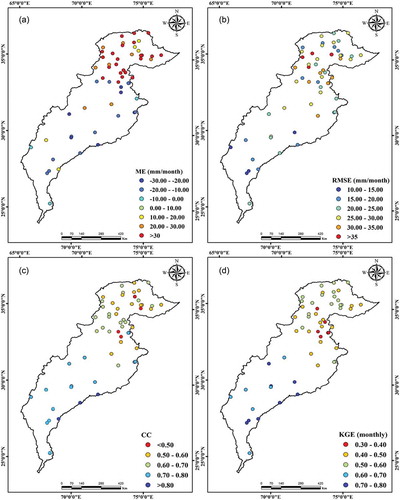
Figure 3. Spatial distribution of daily (a) mean error, (b) root mean square error, (c) correlation coefficient and (d) King-Gupta efficient score in the Indus Basin

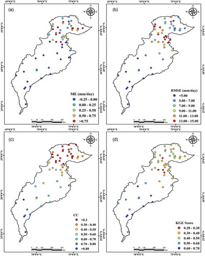
Figure 3(b) presents the RMSE distribution over the study area on a daily scale. The results show a decline in RMSE from north (UIB) to south (LIB) in the study area. There is a mixed distribution pattern over UIB and MIB, and the performance of CHIRPS increases from UIB to LIB. Higher RMSE is observed across UIB, followed by MIB, with a maximum in the northeast of MIB. RMSE in UIB ranges from 3.64 mm/d at RU15 to 14.71 mm/d at RU16. The northeast of MIB receives high and intense precipitation in monsoon followed by pre-monsoon seasons, which contributes to high uncertainties in the region. RMSE in MIB ranges from 4.24 mm/d at RM16 to 13.97 mm/d at RM2. The average RMSE in the UIB and MIB are 13.97 mm/d and 12.32 mm/d. In contrast, a monotonic pattern is observed in the LIB with an average RMSE of 4.97 mm/d.

Figure 3(c) shows the CC of CHIRPS compared to RGs at the point scale. CHIRPS shows relatively low correlation over high elevation; however, CC increases from north to south with a decrease in elevation and precipitation (in both magnitude and intensity). A higher correlation is observed in the LIB (with an average CC of 0.79) while the minimum correlation in UIB (with an average CC of 0.19). Moreover, the highest CC for CHIRPS was observed in LIB (with an average CC of 0.85).

Figure 3(d) presents the spatial distribution of KGE scores for CHIRPS over the Indus Basin against each RG. The results demonstrated the minimum KGE score across UIB and MIB (with the exception of the lower parts). However, the KGE score was significantly increased over the plains regions of MIB and the entire LIB. The maximum/minimum KGE scores for UIB, MIB and LIB are 0.46/0.22 (RU19/RU10), 0.60/0.26 (RM6/RM2) and 0.68/0.53 (RL12/RL7), respectively. The average KGE score for UIB, MIB and LIB is 0.39, 0.47 and 0.58, respectively.

Figure 4 depicts the median POD, FAR and CSI for the five intensity-based daily precipitation classes suggested by Zambrano-Bigiarini et al. (2017). POD and CSI have higher values across the downstream plains areas of MIB and the entire LIB, while lower values are seen in the high-elevation areas of UIB and MIB. The results show that CHIRPS has high POD values (0.71/0.72 in UIB, 0.74/0.81 in MIB and 0.83/0.87 in LIB) for no rain (0–1 mm/d) and moderate rain (5–20 mm/d) events. The lowest values (0.42/0.34 in UIB, 0.54/0.41 in MIB and 0.62/0.53 in LIB) are obtained for heavy rain (20–40 mm/d) and violent rain (≥40 mm/d) events. A similar trend was observed for CSI with higher values (0.74/0.66 in UIB, 0.79/0.71 in MIB and 0.89/0.77 in UIB) during no rain and moderate rain events. The minimum values for CSI were observed in heavy rain events with 0.44, 0.51 and 0.60 in UIB, MIB and LIB, respectively. However, CSI increased in the violent rain events with values of 0.56, 0.64 and 0.71 in UIB, MIB and LIB, respectively. On the other hand, FAR shows consistency with POD, depicting the worst performance of CHIRPS in heavy rain and violent rain events and the best performance during no rain and moderate rain events. The median values of FAR during no rain/moderate rain events across UIB, MIB and LIB are 0.37/0.35, 0.31/0.25 and 0.26/0.18, respectively. Similarly, the median values of FAR during heavy rain/violent rain events are 0.69/0.78, 0.55/0.72 and 0.44/0.56 across UIB, MIB and LIB, respectively.

Figure 4. Median values of (a) probability of detection, (b) False alarm ratio and (c) Critical success index at five classes of precipitation intensity (in mm/d)

4.1.2 Monthly analysis

Figure 5(a) shows the distribution of ME on the monthly time scale. The results reveal that CHIRPS highly overestimated the precipitation in UIB. The highest magnitude of ME (+48.18 mm/month) was observed at RU26, while the lowest (+19.39 mm/month) was observed at RU5. However, a mixed trend of ME distribution was observed in the MIB, which shows both overestimation and underestimation in the same region based on differences in elevation and precipitation magnitude/intensity. CHIRPS overestimated the precipitation in the centre and west, and underestimated it in the eastern MIB. The maximum and minimum overestimation are observed at RM11 (+28.64 mm/month) and RM15 (+12.24 mm/month), respectively. Similarly, the maximum and minimum underestimation in LIB were observed at RL4 (−17.36 mm/month) and RL8 (−4.76 mm/month), respectively.

Figure 5. Spatial distribution of monthly (a) mean error, (b) root mean square error, (c) correlation coefficient and (d) King-Gupta efficient score in the Indus Basin

The monthly distribution of RMSE over the Indus Basin is shown in Fig. 5(b). The figure shows that CHIRPS performance was higher over the plains and low-elevation zones (with low precipitation magnitude and intensity) compared to high elevations (UIB and upstream of MIB characterized by snow and high-intensity/magnitude precipitation, respectively). Considering the UIB, CHIRPS performance is lower in the west with a higher RMSE of 43.89 mm/month at RU21, followed by RU24 with an RMSE of 40.80 mm/month. The RMSE trend in UIB is decreasing towards the east with RMSE ranging from 20 to 26 mm/month. In the MIB, RMSE decreases from west to east and north to south. The maximum RMSE was observed at RM5 (29.58 mm/month), and the minimum RMSE was seen at RM15 (23.72 mm/month). RMSE further decreases in magnitude from MIB to LIB, where the maximum and minimum RMSE values in the LIB were 16.84 and 9.55 mm/month at RL2 and RL10, respectively.

Figure 5(c) shows the spatial distribution of CC at a monthly time scale. The figure shows a lower correlation in the UIB and a high correlation in the LIB. Considering the UIB, a lower CC value was observed at MU8 (0.43) while a higher CC was observed at MU21 (0.68). In the MIB, CHIRPS performance is relatively higher compared to UIB. Higher (0.77) and lower (0.48) CC in the MIB were observed at RM16 and RM7, respectively. However, in the LIB, CHIRPS performance is higher compared to the UIB and MIB. The maximum (0.88) and minimum (0.72) CC in LIB were observed at RL9 and RL1, respectively.

Figure 5(d) depicts the spatial distribution of KGE score on a monthly temporal scale. A similar trend to the previous statistical metrics was observed in the case of KGE score, i.e. a lower KGE score in UIB, followed by MIB, and the highest score in LIB. The regional trend observed in UIB was a relatively higher KGE score in the west and lower values in the east and the extreme southeast. The maximum (0.56) and minimum (0.32) KGE scores were obtained at RU16 and RU11. The average regional KGE score for UIB was 0.44. Similarly, the lowest KGE score for MIB was observed in the extreme northeast of MIB. The KGE score in MIB ranged from 0.35 at RM7 to 0.70 at RM11. The regional average KGE score for MIB was 0.57. LIB depicted the highest performance of CHIRPS in terms of KGE score, where KGE ranged from 0.64 (at RL2) to 0.79 (at RL10), with a regional average of 0.70.

4.1.3 Annual analysis

CHIRPS is also evaluated on an annual scale to analyse its complete performance. Figure 6(a) presents the spatial distribution of annual ME for CHIRPS over the Indus Basin against each RG. The annual distribution shows high ME in the UIB, decreasing towards the LIB (south of the Indus Basin). Overall, the ME in the UIB is higher at RU24, RU29, RU26 and RU22, with values of 588.73, 551.23, 523.29 and 509.84 mm/year, respectively. The minimum ME, of 191.47 mm/year, is observed at MU8. In the case of MIB, the precipitation is overestimated in the upstream of the MIB (positive ME), and tends towards underestimation in the south (downstream) of the MIB. The ME ranges from +387.55 mm/year (north of the MIB) to −272.46 mm/year (south of MIB). Similar to the daily and monthly temporal scale evaluation, CHIRPS slightly underestimated the precipitation in LIB on the annual time scale. Relatively higher underestimation was observed in the northeast of the LIB (−217.15 mm/year), which decreased to −71.35 mm/year in the south of the LIB. Generally, higher performance of CHIRPS was observed in the plains areas (slight overestimation/underestimation), while it highly overestimated the precipitation in the mountainous/glacial regions.

Figure 6. Spatial distribution of annual (a) mean error, (b) root mean square error, (c) correlation coefficient and (d) King-Gupta efficient score in the Indus Basin

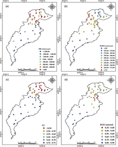
Figure 6(b) presents the regional RMSE distribution at an annual time scale. A similar trend to daily and monthly spatial distribution was observed in the assessment of annual RMSE. CHIRPS shows high performance in the LIB, with RMSE ranging from less than 255 mm/year to 285 mm/year. A mixed distribution was observed in the MIB, where the northwest experienced high RMSE (ranging from 375 to 330 mm/year). Comparatively lower RMSE was observed in the northeast of the MIB (varying from 360 to 300 mm/year). Moreover, RMSE decreased towards the south of MIB (from 330 to 270 mm/year). CHIRPS performed poorly in the UIB, experiencing high RMSE, especially in the northwest and west. The extreme north had a relatively lower RMSE (270 to 300 mm/year) compared to the rest of the UIB. Overall, CHIRPS performance increased with a decrease in elevation and precipitation magnitude/intensity.

Figure 6(c) presents the spatial distribution of annual CC. There was no high variation in CC across MIB and LIB, while UIB experienced significant variation. In the UIB, CC ranged from less than 0.5 in the north to 0.6 in the south. Figure 6(d) depicts the spatial distribution of KGE score on an annual temporal scale. The figure shows significant variations in KGE score across UIB and MIB. It ranged from a minimum of 0.33 at RU31 to a maximum of 0.64 at RU15. The regional average KGE score for UIB was 0.49. Similarly, the trend of KGE score in MIB was minimum in the extreme northeast and maximum towards the south/southwest. The minimum and maximum KGE scores in MIB were 0.36 at RM2 and 0.77 at RM11, with a regional average score of 0.58. The KGE score was highest in LIB, ranging from 0.71 at RL3 to 0.89 at RL10. The average regional KGE score for LIB was 0.80.

4.1.4 Seasonal performance of CHIRPS

The performance of CHIRPS is comprehensively assessed during different climatic seasons over the Indus Basin, Pakistan. The climate of the Indus Basin is divided into four seasons, i.e. winter (December–March), pre-monsoon (April–June), monsoon (July–September) and post-monsoon (October–November). The Indus Basin receives most of its precipitation in monsoon season (Rahman et al. 2018). The average daily metrics of CHIRPS at the seasonal scale are presented in Table 4. The results show that during monsoon season, CHIRPS presented the highest ME for UIB and the lowest for LIB. Similar trends were observed for the other seasons, except post-monsoon season. Comparing all seasons, CHIRPS performed well in the winter (low precipitation magnitude/intensity) followed by pre-monsoon. The highest RMSE was observed in UIB during the monsoon season, and the lowest RMSE was observed in LIB during the pre-monsoon season. CHIRPS presented the lowest performance in terms of CC in UIB, and the highest performance was observed in LIB. The overall metrics show that CHIRPS overestimated the seasonal precipitation in UIB, while it underestimated moderate to low precipitation and overestimated heavy precipitation in MIB and LIB.

Table 4. Performance assessment of CHIRPS in the Indus Basin at seasonal scale during 2000–2013

Period	Indices	UIB	MIB	LIB
Pre-monsoon	ME	26.7	15.5	8.3
	RMSE	38.1	29.8	14.6
	CC	0.43	0.65	0.74
Monsoon	ME	43.2	34.1	14.2
	RMSE	48.5	25.3	20.5
	CC	0.48	0.63	0.71
Post-monsoon	ME	21.4	−10.3	−20.4
	RMSE	27.3	19.2	24.5
	CC	0.59	0.68	0.76
Winter	ME	15.2	−11.4	−23.5
	RMSE	28.2	23.6	20.2
	CC	0.64	0.72	0.79

4.2 Comparison of CHIRPS v. 2.0 with TMPA_3B42 v. 7 and IMERG V06

The performance of CHIRPS on a daily and monthly temporal scale is compared with extensively evaluated SPD across Pakistan, i.e. TRMM TMPA (hereinafter TMPA) 3B42 v. 7 for daily and 3B43 v. 7 for monthly scale comparison. The performance is also compared with IMERG V06 (hereinafter IMERG) on daily and monthly temporal scales. TMPA was selected as many studies have confirmed its better performance over Pakistan (Cheema and Bastiaanssen 2012, Anjum et al. 2016, Hussain et al. 2018, Iqbal and Athar 2018). However, IMERG has outperformed TMPA across all climate regions overall (Ullah et al. 2019, Rahman and Shang 2020). Therefore, the extensive evaluation of CHIRPS against both state-of-the-art SPDs (TMPA and IMERG) will help readers understand the spatial and temporal performance and potential/limitations of CHIRPS.

Figures 7 and 8 show the differences in precipitation values of CHIRPS with RGs, TMPA and IMERG on daily and monthly temporal scales across the UIB, MIB and LIB. Overall, IMERG outperformed both CHIRPS and TMPA across all climate regions at both daily and monthly temporal scales (shown in column scatter plots). On one hand, all the SPDs overestimated the precipitation across UIB. CHIRPS depicted high overestimation, followed by TMPA and IMERG evaluated at daily temporal scale. At the majority of stations in UIB, the performance of CHIRPS is comparable with that of TMPA. On the other hand, all the SPDs underestimated precipitation in MIB and LIB. IMERG dominated CHIRPS and TMPA, having close estimates to RGs. Overall, it can be concluded that at the daily temporal scale, CHIRPS outperformed the TMPA in MIB and LIB (plains areas with low precipitation magnitude and intensity) while TMPA’s performance is relatively better in the UIB (mountainous and glacial areas with high precipitation magnitude and intensity). Detailed information about SPDs’ poor performance in UIB can found in Rahman et al. (2020c).

Figure 7. Comparison of Climate Hazard Group InfraRed Precipitation Satellite with Multi-Satellite Precipitation Analysis 3B42 v. 7 and Global Precipitation Measurement-based Integrated Multi-Satellite Retrievals for GPM at a daily temporal scale in (a) Upper Indus Basin, (b) Middle Indus Basin and (c) Lower Indus Basin

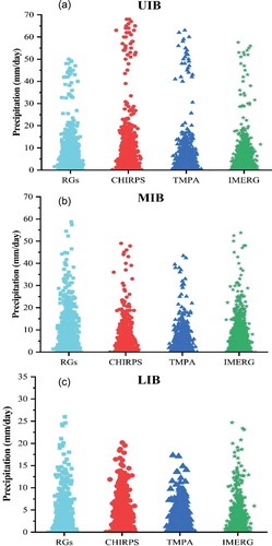
Figure 8. Comparison of Climate Hazard Group InfraRed Precipitation Satellite with Multi-Satellite Precipitation Analysis 3B43 v. 7 and Global Precipitation Measurement-based Integrated Multi-Satellite Retrievals for GPM at a monthly temporal scale in (a) Upper Indus Basin, (b) Middle Indus Basin and (c) Lower Indus Basin

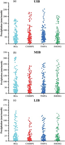
Figure 8 shows the column scatter plots that compare the performance of CHIRPS against RGs, TMPA and IMERG on monthly time scale. CHIRPS and TMPA have comparable precipitation estimates, i.e. the monthly average precipitation according to CHIRPS and TMPA in UIB is 63 and 68 mm/month, respectively. However, IMERG outperformed both CHIRPS and TMPA, with an average monthly precipitation of 59 mm/month compared to the RGs (53 mm/month). MIB and LIB also depicted the superiority of IMERG, while CHIRPS and TMPA have comparable precipitation estimates.

Figure 9 depicts the comparison of CHIRPS against IMERG and TMPA based on ME, RMSE, CC, POD, FAR and CSI on daily temporal scales across UIB, MIB and LIB. The violin plots with quartiles show three lines, i.e. the 25% and 75% quartiles are represented by the bottom and top lines, respectively, while the middle line shows the median of each statistical metric. It can be seen that in UIB, TMPA has relatively lower ME and RMSE compared to CHIRPS. However, IMERG outperformed both CHIRPS and TMPA in terms of ME and RMSE in UIB. ME and RMSE decrease when we propagate from UIB to MIB and then LIB. A similar trend was observed on a monthly scale for ME and RMSE (Figure 10). Figure 9 shows the CC of CHIRPS is lower than that of both IMERG and TMPA. CHIRPS has a wide range of CC (0.12 to 0.55) in UIB, with most CC values around 0.24, compared to TMPA (0.25 to 0.48) and IMERG (0.29 to 0.64). The median for TMPA and IMERG lies in the range of 0.23–0.26 and 0.37–0.42, respectively. However, the CC for CHIRPS is higher in the other basins, particularly in LIB. The performance of CHIRPS and TMPA is comparable in MIB with median CC values of 0.52 and 0.49. IMERG outperformed both CHIRPS and TMPA across all Indus sub-basins. CC is significantly increased on the monthly time scale compared to the daily temporal scale for all basins (Fig. 10). In UIB, CC ranges from 0.43 to 0.68 for CHIRPS and 0.42 to 0.58 for TMPA. In MIB, CC ranges from 0.48 to 0.77 for CHIRPS and 0.53 to 0.69 for TMPA, while in LIB, CC ranges from 0.72–0.88 for CHIRPS and 0.54–0.77 for TMPA. On the other hand, CC for IMERG across UIB, MIB and LIB ranges from 0.60 to 0.77, 0.68 to 0.85 and 0.83 to 0.94, respectively. A comparison of POD, FAR and CSI is also shown in Fig. 9. Overall, IMERG outperformed both CHIRPS and TMPA across UIB, MIB and LIB. However, the performance of CHIRPS is better than that of TMPA across MIB and LIB, while TMPA dominated CHIRPS in UIB.

Figure 9. Daily statistical matrices for Climate Hazard Group InfraRed Precipitation Satellite, Multi-Satellite Precipitation Analysis and Global Precipitation Measurement-based Integrated Multi-Satellite Retrievals for GPM across Upper Indus Basin, Middle Indus Basin and Lower Indus Basin

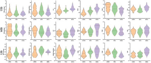
Figure 10. Monthly statistical matrices for Climate Hazard Group InfraRed Precipitation Satellite, Multi-Satellite Precipitation Analysis and Global Precipitation Measurement-based Integrated Multi-Satellite Retrievals for GPM across Upper Indus Basin, Middle Indus Basin and Lower Indus Basin

4.3 Hydrological evaluation of CHIRPS

The performance of CHIRPS is assessed in two sub-basins of the Indus Basin, i.e. UIB (Gilgit Basin) and MIB (Soan Basin). Overall, the analyses depicted relatively poor performance of CHIRPS in UIB and moderate performance in MIB. Five iterations were performed to determine the most sensitive parameters for both sub-basins. The sensitivity analyses identified 14 and eight sensitive parameters for Gilgit and Soan River sub-basins, respectively. The sensitive parameters for both sub-basins are presented in Tables 2 and 3, respectively. Model calibration and validation were performed for 2005–2007 and 2008–2010, respectively.

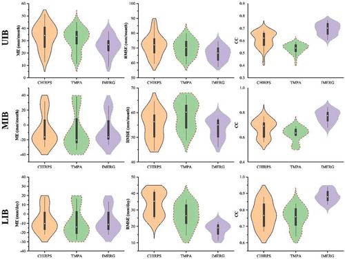
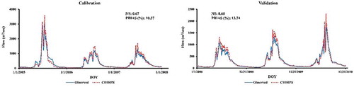
SWAT was calibrated and validated across Gilgit Basin (Fig. 11) using the precipitation data from CHIRPS, while the remaining climate data used is the observed data acquired from PMD and WAPDA. The results depict good performance (NS = 0.67 and PBIAS = 10.37%) during calibration and satisfactory/good performance (NS = 0.60/PBIAS = 13.74) during the validation period. Overall, the results showed that CHIRPS has overestimated the streamflow across the glacial sub-basins of UIB.

Figure 11. Calibration (2005–2007) and validation (2008–2010) of the SWAT model using Climate Hazard Group InfraRed Precipitation Satellite precipitation data across the Gilgit Basin

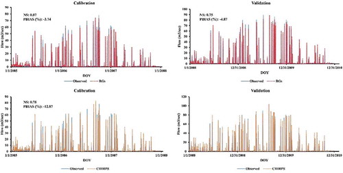
Figures 12 and 13 compare the simulated and observed daily streamflow from RGs and CHIRPS datasets at Chirah and Sill river stations during the calibration (2005–2007) and validation (2008–2010) periods. The hydrographs developed using RGs showed reasonable agreement while CHIRPS (which mostly overestimated streamflow) presented satisfactory to good results. Using the RG precipitation data, the SWAT model performed best in simulating streamflow, with NS and PBIAS of 0.88 and +9.4% during calibration and 0.79 and +6.59% during validation at Chirah station. Similarly, the values were 0.87 and 0.75 for NS, and −3.74% and −4.87% for PBIAS, at Sill River station. This demonstrates very good performance of the simulations according to criteria specified by Moriasi et al. (2007). However, CHIRPS produced satisfactory to good performance in streamflow simulations at both flow gauges. The NS/PBIAS values for CHIRPS-simulated streamflow at Chirah station during the calibration and validation periods were 0.73/−13.75% and 0.63/−17.35%, respectively. Similarly, for Sill River station, the NS/PBIAS values for CHIRPS were 0.78/−12.87% and 0.70/−16.04% during the calibration and validation periods, respectively.

Figure 12. Calibration (2005–2007) and validation (2008–2010) of the SWAT model using Raingauges and Climate Hazard Group InfraRed Precipitation Satellite precipitation data at Chirah station

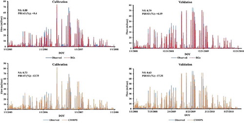
Figure 13. Calibration (2005–2007) and validation (2008–2010) of the SWAT model using Raingauges and Climate Hazard Group InfraRed Precipitation Satellite precipitation data at Sill station

5 Discussion and conclusions

Precipitation is the main component of the hydrological cycle, and its accurate estimation is a challenging task, especially in poorly gauged/ungauged regions. Due to the availability of different SPDs, precipitation estimation on a regional and global scale is now convenient. However, for better application, the evaluation of SPDs is indispensable. For effective planning and management of water resources in the Indus Basin of Pakistan, where the Indus River is the primary water supply source for a large population, it is essential to precisely estimate the precipitation data. Therefore, CHIRPS was extensively evaluated in the current study at daily, monthly and annual temporal scales across the Indus Basin. The basin was divided into three sub-basins, i.e. UIB, MIB and LIB. The performance of CHIRPS was comprehensively evaluated against 59 RGs obtained from PMD and WAPDA. Moreover, CHIRPS was compared with state-of-the-art SPDs, TMPA (3B42 and 3B43 v. 7) and IMERG (V06), at daily and monthly time scales.

Due to the fine spatiotemporal resolution of CHIRPS, it has been recommended by several studies for hydrological analysis and water resource management (Katsanos et al. 2016, Paredes-Trejo et al. 2017, Bai et al. 2018, Gao et al. 2018, Saeidizand et al. 2018). Therefore, the hydrological utility of CHIRPS was tested in two sub-basins of Indus Basin, i.e. Gilgit (UIB) and Soan (MIB) basins. The SWAT model was used to assess the performance of CHIRPS in simulating daily streamflow across Gilgit and Soan basins, which have completely different climates.

CHIRPS has been evaluated in different regions around the world (Dinku et al. 2018, Gebrechorkos et al. 2018, Prakash 2019, Wu et al. 2019), and particularly across Pakistan (Ullah et al. 2019, Nawaz et al. 2021). Wu et al. (2019) employed 122 RGs to assess the performance of CHIRPS in Yunnan Province of China using a point-to-pixel approach. They obtained good results at monthly and annual temporal scales but relatively low performance at the daily time scale. Dinku et al. (2018) used a pixel-to-pixel approach to evaluate CHIRPS performance in East Africa at daily, monthly, and decadal time scales and reported better performance. Similarly, Prakash (2019) compared CHIRPS against SM2RAIN-CCI (Soil Moisture to RAIN - Climate Change Initiative) and TMPA across India and reported satisfactory performance. The performance of CHIRPS has also been evaluated in Nepal and Bhutan, and it was found to be relatively poor for high-elevation regions and heavy precipitation seasons (Khandu et al. 2016, Shrestha et al. 2017).

Very few studies have evaluated the performance of CHIRPS over Pakistan (Ullah et al. 2019 and Nawaz et al. 2021). Such a detailed assessment (in terms of both time scale and hydrological assessment) is the unique feature of the current study. Our results demonstrate that CHIRPS overestimated the precipitation over high-elevation regions while underestimating it in plains areas. Moreover, the seasonal evaluation of CHIRPS shows that CHIRPS overestimated the precipitation with high magnitude during monsoon season. The performance was significantly better in winter compared to the other seasons. Further, CHIRPS depicted satisfactory performance at the daily temporal scale, which improved for monthly and annual time scales. Daily precipitation estimates from CHIRPS showed relatively high errors in UIB, which is mostly a glacial region and situated at high elevations. The findings from the current study are supported by Ullah et al. (2019) and Nawaz et al. (2021). Both studies reported that moonsoon precipitation is significant in the north and central parts of the country. However, a decreasing pattern has been observed for the southern parts, and these findings are consistent with the monthly results of the present study. Ullah et al. (2019) demonstrated the dependency (on magnitude of precipitation) of CHIRPS on a seasonal scale, which supports the findings of current study.

Ullah et al. (2019) also evaluated the potential of CHIRPS and TMPA over Pakistan at daily, monthly and annual scales. They concluded that CHRPS and TMPA showed similar precipitation trends for moonsoon and winter seasons. This finding is consistent with the present study, where it is concluded that CHIRPS and TMPA have very similar performances across different regions of the Indus Basin. On a regional scale, IMERG dominated the SPDs across all sub-basins of the Indus Basin, while TMPA outperformed CHIRPS in UIB (particularly in the glacial zone). However, the performance of CHIRPS increased significantly in the mid- to low-elevation regions (MIB to LIB) and dominated over that of TMPA. Other studies conducted in the Indus Basin found similar trends for TMPA in the UIB (Khan et al. 2014, Anjum et al. 2016, Hussain et al. 2018, Iqbal and Athar 2018, Rahman et al. 2018, 2019, Ullah et al. 2019, Satgé et al. 2021).

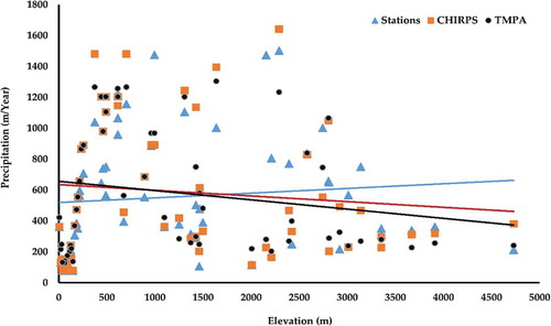
The overestimated precipitation for UIB may have occurred a number of reasons, including climatic condition, topography, seasonality, wind effect and sparse distribution of meteorological stations. Previous studies concluded that precipitation is sensitive to topographic elevation (Hughes et al. 2009, Dinku et al. 2010, Kumari et al. 2017, Ren et al. 2018) – although precipitation and elevation have a unique relationship for every region. Figure 14 shows the relationship between RG elevation and mean annual precipitation from SPDs and RGs. The results show that station elevation is slightly positively correlated with RG data, and it is negatively correlated with CHIRPS and TMPA data.

Figure 14. Comparison of mean annual precipitation of Raingauges and SPDS at different elevations. The lines represent the trend of precipitation with elevation

Several studies have evaluated the hydrological utility of CHIRPS using the SWAT model in different basins around the world (Tuo et al. 2016, Bayissa et al. 2017; Duan et al. 2019). Tuo et al. (2016) reported satisfactory performance when CHIRPS was used to simulate monthly streamflow. Similarly, Duan et al. (2019) evaluated the performance of CHIRPS against TMPA and Climate Forecast System Reanalysis (CFSR) in simulating streamflow on daily and monthly time scales across Gilgel Abay Basin, Ethiopia. CHIRPS produced satisfactory results compared to other SPDs. However, higher accuracy of CHIRPS was observed in the Upper Blue Nile Basin compared to the other four SPDs (Bayissa et al. 2017). The current study found satisfactory performance of CHIRPS in the Gilgit Basin (streamflow was mostly overestimated) and satisfactory to good performance in simulating the daily streamflow in the Soan Basin. The comparison between streamflow simulated using RGs and CHIRPS as input showed that CHIRPS underestimated the streamflow in Soan Basin. The underestimation occurred during the monsoon season, when CHIRPS was unable to accurately capture precipitation, which can be considered a major reason for the low NS values.

There might be a number of reasons behind the performance dependency (both spatial and temporal) of SPDs, and therefore, identifying the main sources of the errors is a challenging task. Moreover, the sources of errors may vary spatially (depending on the division of climate regions, topography, elevation, vegetation cover, etc.) and temporally (seasonality, intensity, time scale) (Ayehu et al. 2018). The lower parts of UIB and the upstream part of MIB receive intense precipitation in monsoon season (Jilani et al. 2008, Rahman et al. 2020b, 2020c) due to the western disturbance and precipitation from the Bay of Bengal (Asmat and Athar 2017, Iqbal and Athar 2018). Therefore, the high magnitude of error in IMERG, TMPA and CHIRPS may be due to the variability of localized precipitation. The underestimation in MIB and LIB could be due to instrument error because intense precipitation scatters the radio frequency.

The present study has several limitations that are worth mentioning. Due to the limited number of RGs, the performance assessment of SPDs at the sub-basin scale could produce uncertain results. The same applies to the point-to-pixel analysis, where the point-based data is compared with a pixel, and hydrological modelling has been performed. These comparisons cannot be considered fair; therefore, it is suggested to use multiple precipitation datasets for hydrological modelling, which will be helpful for better simulation of streamflow. However, we have tried to compare the hydrological analyses of CHIRPS across two different climate regions, i.e. UIB and MIB, to develop a thorough understanding of CHIRPS’ behaviour with respect to precipitation intensity, climate variability, topography, etc. CHIRPS produced different results when evaluated across Gilgit Basin (which is situated in the glacial region) and Soan Basin (having a humid to semi-humid nature). The reasons behind the satisfactory (Gilgit Basin) to good (Soan Basin) performance might be a limited number of RGs for calibration and validation of the SWAT model (Rahman et al. 2020a), snow and glacier impact on streamflow (Tuo et al. 2018), complex topography or climate change (Lettenmaier et al. 2015, Huss and Hock 2018). Moreover, the selection of sensitive parameters plays a critical role, and this selection changes from region to region and with the type of input datasets. Therefore, it is suggested to calibrate and validate different datasets separately so that the sensitivity of parameters can be well tested.

Acknowledgements

We acknowledge PMD and WAPDA for their support in providing RG precipitation data, and express our gratitude to the SPD developers. We thank the anonymous reviewers, whose valuable and constructive comments helped to improve the quality of this article.

Disclosure statement

No potential conflict of interest was reported by the authors.

References

- Abbaspour, K., 2015. SWAT-CUP 2012: SWAT calibration and uncertainty programs: a user manual. Duebendorf, Switzerland: Department of Systems Analysis, Integrated Assessment and Modelling (SIAM), Eawag, Swiss Federal Institute of Aquatic Science and Technology.
- Abbaspour, K.C., et al. 2007. Modelling hydrology and water quality in the pre-alpine/ alpine Thur watershed using SWAT. Journal of Hydrology, 333 (2–4), 413–430. doi:https://doi.org/10.1016/j.jhydrol.2006.09.014.
- Abbaspour, K.C., et al., 2015. A continental-scale hydrology and water quality model for Europe: Calibration and uncertainty of a high-resolution large-scale SWAT model. Journal of Hydrology, 524, 733–752.
- Abbaspour, K.C., Johnson, C.A., and Genuchten, M.T.V., 2004. Estimating uncertain flow and transport parameters using a sequential uncertainty fitting procedure. Vadose Zone Journal, 3 (4), 1340–1352. doi:https://doi.org/10.2136/vzj2004.1340.
- Anjum, M.N., et al., 2016. Evaluation of high-resolution satellite-based real-time and post-real-time precipitation estimates during 2010 extreme flood event in Swat River Basin, Hindukush region. Advances in Meteorology, 2016.
- Arnold, J.G., et al., 1998. Large area hydrologic modeling and assessment part I: model development. Journal of the American Water Resources Association, 34 (1), 73–89. doi:https://doi.org/10.1111/j.1752-1688.1998.tb05961.x.
- Asmat, U. and Athar, H., 2017. Run-based multi-model interannual variability assessment of precipitation and temperature over Pakistan using two IPCC AR4-based AOGCMs. Theoretical and Applied Climatology, 127 (1–2), 1–6. doi:https://doi.org/10.1007/s00704-015-1616-6.
- Ayehu, G.T., et al., 2018. Validation of new satellite rainfall products over the Upper Blue Nile Basin, Ethiopia. Atmospheric Measurement Techniques, 11 (4), 1921–1936. doi:https://doi.org/10.5194/amt-11-1921-2018.
- Bai, L., et al., 2018. Accuracy of chirps satellite-rainfall products over mainland China. Remote Sensing, 10 (3), 362. doi:https://doi.org/10.3390/rs10030362.
- Balkhair, K.S. and Ur Rahman, K. 2019. Development and assessment of rainwater harvesting suitability map using analytical hierarchy process, GIS, and RS techniques. Geocarto International, 36, 1–19. just-accepted.
- Bayissa, Y., et al., 2017. Evaluation of satellite-based rainfall estimates and application to monitor meteorological drought for the Upper Blue Nile Basin, Ethiopia. Remote Sensing, 9 (7), 669. doi:https://doi.org/10.3390/rs9070669.
- Bitew, M. and Gebremichael, M., 2011. Assessment of satellite rainfall products for streamflow simulation in medium watersheds of the Ethiopian highlands. Hydrology and Earth System Sciences, 15 (4), 1147–1155. doi:https://doi.org/10.5194/hess-15-1147-2011.
- Cheema, M.J.M. and Bastiaanssen, W.G., 2012. Local calibration of remotely sensed rainfall from the TRMM satellite for different periods and spatial scales in the Indus Basin. International Journal of Remote Sensing, 33 (8), 2603–2627. doi:https://doi.org/10.1080/01431161.2011.617397.
- Chiaravalloti, F., et al., 2018. Assessment of GPM and SM2RAIN-ASCAT rainfall products over complex terrain in southern Italy. Atmospheric Research, 206, 64–74. doi:https://doi.org/10.1016/j.atmosres.2018.02.019
- Dimri, A.P., et al., 2015. Western disturbances: a review. Reviews of Geophysics, 53 (2), 225–246. doi:https://doi.org/10.1002/2014RG000460.
- Dinku, T., et al., 2007. Validation of satellite rainfall products over East Africa’s complex topography. International Journal of Remote Sensing, 28 (7), 1503–1526. doi:https://doi.org/10.1080/01431160600954688.
- Dinku, T., et al., 2018. Validation of the CHIRPS satellite rainfall estimates over eastern Africa. Quarterly Journal of the Royal Meteorological Society, 144 (S1), 292–312. doi:https://doi.org/10.1002/qj.3244.
- Dinku, T., Connor, S.J., and Ceccato, P., 2010. Comparison of CMORPH and TRMM-3B42 over mountainous regions of Africa and South America. In: Satellite rainfall applications for surface hydrology. Dordrecht: Springer, 193–204.
- Duan, Z., et al., 2019. Hydrological evaluation of open-access precipitation and air temperature datasets using SWAT in a poorly gauged Basin in Ethiopia. Journal of Hydrology, 569, 612–626. doi:https://doi.org/10.1016/j.jhydrol.2018.12.026.
- Ebert, E.E., Janowiak, J.E., and Kidd, C., 2007. Comparison of near-real-time precipitation estimates from satellite observations and numerical models. Bulletin of the American Meteorological Society, 88 (1), 47–64. doi:https://doi.org/10.1175/BAMS-88-1-47.
- Eckstein, D., Künzel, V., and Schäfer, L., 2017. Global climate risk index 2018. Bonn: Germanwatch.
- Funk, C.C., et al., 2014. A quasi-global precipitation time series for drought monitoring. US Geological Survey Data Series, 832, 4.
- Gao, F., et al., 2018. Evaluation of CHIRPS and its application for drought monitoring over the Haihe River Basin, China. Natural Hazards, 92 (1), 155–172. doi:https://doi.org/10.1007/s11069-018-3196-0.
- Gassman, P.W., et al., 2007. The soil and water assessment tool: historical development, applications, and future research directions. Transactions of the ASABE, 50 (4), 1211–1250. doi:https://doi.org/10.13031/2013.23637.
- Gebere, S.B., et al., 2015. Performance of high resolution satellite rainfall products over data scarce parts of Eastern Ethiopia. Remote Sensing, 7 (9), 11639–11663. doi:https://doi.org/10.3390/rs70911639.
- Gebrechorkos, S.H., Hülsmann, S., and Bernhofer, C., 2018. Evaluation of multiple climate data sources for managing environmental resources in East Africa. Hydrology and Earth System Sciences, 22 (8), 4547–4564. doi:https://doi.org/10.5194/hess-22-4547-2018.
- Green, W.H. and Ampt, G.A., 1911. Studies on soil physics. Journal of Agricultural Science, 4 (1), 11–24.
- Guo, H., et al., 2016. Evaluation of PERSIANN-CDR for meteorological drought monitoring over China. Remote Sensing, 8 (5), 379. doi:https://doi.org/10.3390/rs8050379.
- Guo, H., et al., 2017. Meteorological drought analysis in the Lower Mekong Basin using satellite-based long-term CHIRPS product. Sustainability, 9 (6), 901. doi:https://doi.org/10.3390/su9060901.
- Gupta, H.V., et al., 2009. Decomposition of the mean squared error and NSE performance criteria: implications for improving hydrological modelling. Journal of Hydrology, 377 (1–2), 80–91. doi:https://doi.org/10.1016/j.jhydrol.2009.08.003.
- Huard, D. and Mailhot, A., 2008. Calibration of hydrological model GR2M using Bayesian uncertainty analysis. Water Resources Research, 44 (2), 2. doi:https://doi.org/10.1029/2007WR005949.
- Huffman, G.J., et al., 2018. NASA Global Precipitation Measurement (GPM) Integrated Multi-satellitE Retrievals for GPM (IMERG); Algorithm Theoretical Basis Document (ATBD) Version 5.2; NASA/GSFC:. Greenbelt, MD, USA.
- Huffman, G.J., Bolvin, D.T., and Nelkin, E.J., 2015. Day 1 IMERG final run release notes. Greenbelt, MD, USA: NASA/GSFC.
- Hughes, M., Hall, A., and Fovell, R.G., 2009. Blocking in areas of complex topography, and its influence on rainfall distribution. Journal of the Atmospheric Sciences, 66 (2), 508–518. doi:https://doi.org/10.1175/2008JAS2689.1.
- Huss, M. and Hock, R., 2018. Global-scale hydrological response to future glacier mass loss. Nature Climate Change, 8 (2), 135–140. doi:https://doi.org/10.1038/s41558-017-0049-x.
- Hussain, Y., et al., 2018. Performance of CMORPH, TMPA, and PERSIANN rainfall datasets over plain, mountainous, and glacial regions of Pakistan. Theoretical and Applied Climatology, 131 (3–4), 1119–1132. doi:https://doi.org/10.1007/s00704-016-2027-z.
- Iqbal, M.F. and Athar, H., 2018. Validation of satellite based precipitation over diverse topography of Pakistan. Atmospheric Research, 201, 247–260. doi:https://doi.org/10.1016/j.atmosres.2017.10.026
- Jilani, R., et al., 2008 Nov. Revalidation of TRMM precipitation data with ground based measurements for selected cities of Pakistan. In Asian Conference on Remote Sensing (ACRS), Colombo, Sri Lanka, Vol. 1.
- Kalair, A., et al., 2019. Water, energy and food nexus of indus water treaty: water governance. Water-Energy Nexus.
- Katsanos, D., Retalis, A., and Michaelides, S., 2016. Validation of a high-resolution precipitation database (CHIRPS) over Cyprus for a 30-year period. Atmospheric Research, 169, 459–464. doi:https://doi.org/10.1016/j.atmosres.2015.05.015
- Khan, M.A., et al., 2016. The challenge of climate change and policy response in Pakistan [journal article]. Environmental Earth Sciences, 75 (5), 412. doi:https://doi.org/10.1007/s12665-015-5127-7.
- Khan, S.I., et al., 2014. Evaluation of three high-resolution satellite precipitation estimates: potential for monsoon monitoring over Pakistan. Advances in Space Research, 54 (4), 670–684. doi:https://doi.org/10.1016/j.asr.2014.04.017.
- Khandu, Awange, J.L., and Forootan, E., 2016. An evaluation of high-resolution gridded precipitation products over Bhutan (1998–2012). International Journal of Climatology, 36 (3), 1067–1087. doi:https://doi.org/10.1002/joc.4402.
- Kidd, C., et al., 2012. Intercomparison of high-resolution precipitation products over northwest Europe. Journal of Hydrometeorology, 13 (1), 67–83. doi:https://doi.org/10.1175/JHM-D-11-042.1.
- Kling, H., Fuchs, M., and Paulin, M., 2012. Runoff conditions in the upper Danube Basin under an ensemble of climate change scenarios. Journal of Hydrology, 424-425, 264–277. doi:https://doi.org/10.1016/j.jhydrol.2012.01.011
- Kumari, M., et al., 2017. Geographically weighted regression based quantification of rainfall–topography relationship and rainfall gradient in Central Himalayas. International Journal of Climatology, 37 (3), 1299–1309. doi:https://doi.org/10.1002/joc.4777.
- Kummerow, C., et al., 1998. The tropical rainfall measuring mission (TRMM) sensor package. Journal of Atmospheric and Oceanic Technology, 15 (3), 809–817. doi:https://doi.org/10.1175/1520-0426(1998)015<0809:TTRMMT>2.0.CO;2.
- Kummerow, C., et al., 2000. The status of the Tropical Rainfall Measuring Mission (TRMM) after two years in orbit. Journal of Applied Meteorology, 39 (12), 1965–1982. doi:https://doi.org/10.1175/1520-0450(2001)040<1965:TSOTTR>2.0.CO;2.
- Laghari, A., Vanham, D., and Rauch, W., 2012. The Indus Basin in the framework of current and future water resources management. Hydrology and Earth System Sciences, 16 (4), 1063. doi:https://doi.org/10.5194/hess-16-1063-2012.
- Lettenmaier, D.P., et al. 2015. Inroads of remote sensing into hydrologic science during the WRR era. Water Resources Research, 51 (9), 7309–7342. doi:https://doi.org/10.1002/2015WR017616.
- Liu, Z., 2015. Comparison of versions 6 and 7 3-hourly TRMM multi-satellite precipitation analysis (TMPA) research products. Atmospheric Research, 163, 91–101. doi:https://doi.org/10.1016/j.atmosres.2014.12.015
- Liviu Giosan, L., et al., 2006. Recent morphodynamics of the Indus delta shore and shelf. Continental Shelf Research, 26 (14), 1668–1684. doi:https://doi.org/10.1016/j.csr.2006.05.009.
- Ma, Y., et al., 2018. Performance of optimally merged multisatellite precipitation products using the dynamic Bayesian model averaging scheme over the Tibetan Plateau. Journal of Geophysical Research: Atmospheres, 123 (2), 814–834.
- Mainali, J. and Pricope, N.G., 2017. High-resolution spatial assessment of population vulnerability to climate change in Nepal. Applied Geography, 82, 66–82. doi:https://doi.org/10.1016/j.apgeog.2017.03.008
- Mapes Kerry, L. and Pricope, N.G., 2020. Evaluating SWAT model performance for runoff, percolation, and sediment loss estimation in low-gradient watersheds of the Atlantic coastal plain. Hydrology, 7 (2), 21. doi:https://doi.org/10.3390/hydrology7020021.
- Mei, Y., et al., 2016. Evaluating satellite precipitation error propagation in runoff simulations of mountainous Basins. Journal of Hydrometeorology, 17 (5), 1407–1423. doi:https://doi.org/10.1175/JHM-D-15-0081.1.
- Mekonnen, D.F., et al., 2018. Analysis of combined and isolated effects of land-use and land-cover changes and climate change on the upper Blue Nile River basin’s streamflow. . Hydrology and Earth System Sciences, 22 (12), 6187–6207. doi:https://doi.org/10.5194/hess-22-6187-2018.
- Moriasi, D.N., et al., 2007. Model evaluation guidelines for systematic quantification of accuracy in watershed simulations. Transactions of the ASABE, 50 (3), 885–900. doi:https://doi.org/10.13031/2013.23153.
- Muhammad, W., et al., 2018. Improving the regional applicability of satellite precipitation products by ensemble algorithm. Remote Sensing, 10 (4), 577. doi:https://doi.org/10.3390/rs10040577.
- Muthuwatta, L.P., et al., 2009. Calibration of a semi-distributed hydrological model using discharge and remote sensing data. IAHS Publication, 333, 52.
- Nair, S., Srinivasan, G., and Nemani, R., 2009. Evaluation of multi-satellite TRMM derived rainfall estimates over a western state of India. Journal of the Meteorological Society of Japan. Ser. II, 87 (6), 927–939. doi:https://doi.org/10.2151/jmsj.87.927.
- Nash, J.E. and Sutcliffe, J.V., 1970. River flow forecasting through conceptual models part I—A discussion of principles. Journal of Hydrology, 10 (3), 282–290.
- Nawaz, M., Iqbal, M.F., and Mahmood, I., 2021. Validation of CHIRPS satellite-based precipitation dataset over Pakistan. Atmospheric Research, 248, 105289. doi:https://doi.org/10.1016/j.atmosres.2020.105289
- Neitsch, S.L., et al., 2011. Soil and water assessment tool theoretical documentation version 2009. Texas Water Resources Institute.
- Nguyen, H.H., et al., 2017a. Modelling the impacts of altered management practices, land use and climate changes on the water quality of the Millbrook catchment-reservoir system in South Australia. . Journal of Environmental Management, 202, 1–11. doi:https://doi.org/10.1016/j.jenvman.2017.07.014
- Nogueira, S.M.C., Moreira, M.A., and Volpato, M.M.L., 2018. Evaluating precipitation estimates from Eta, TRMM and CHRIPS data in the South-Southeast Region of Minas Gerais State—Brazil. Remote Sensing, 10 (3), 313. doi:https://doi.org/10.3390/rs10020313.
- Ochoa-Sánchez, A., et al., 2014. Evaluation of TRMM 3B42 precipitation estimates and WRF retrospective precipitation simulation over the Pacific–Andean region of Ecuador and Peru. Hydrology and Earth System Sciences, 18 (8), 3179–3193. doi:https://doi.org/10.5194/hess-18-3179-2014.
- Paredes-Trejo, F.J., Barbosa, H., and Kumar, T.V., 2017. Validating CHIRPS-based satellite precipitation estimates in Northeast Brazil. Journal of Arid Environments, 139, 26–40. doi:https://doi.org/10.1016/j.jaridenv.2016.12.009
- Pathak, J., 2012. Measuring glacier change in the Himalayas. UNEP Global Environmental Alert service (GEAS).
- Pierre, C., et al., 2011. Pluriannual comparisons of satellite-based rainfall products over the Sahelian belt for seasonal vegetation modeling. Journal of Geophysical Research: Atmospheres, 116 (D18), D18. doi:https://doi.org/10.1029/2011JD016115.
- Prakash, S., et al., 2014. An evaluation of high-resolution multisatellite rainfall products over the Indian monsoon region. International Journal of Remote Sensing, 35 (9), 3018–3035. doi:https://doi.org/10.1080/01431161.2014.894661.
- Prakash, S., 2019. Performance assessment of CHIRPS, MSWEP, SM2RAIN-CCI, and TMPA precipitation products across India. Journal of Hydrology, 571, 50–59. doi:https://doi.org/10.1016/j.jhydrol.2019.01.036
- Price, K., et al., 2014. Comparison of radar and gauge precipitation data in watershed models across varying spatial and temporal scales. Hydrological Processes, 28 (9), 3505–3520. doi:https://doi.org/10.1002/hyp.9890.
- Rahman, K.U., et al., 2018. Developing an ensemble precipitation algorithm from satellite products and its topographical and seasonal evaluations over Pakistan. Remote Sensing, 10 (11), 1835. doi:https://doi.org/10.3390/rs10111835.
- Rahman, K.U., et al., 2020a. Hydrological evaluation of merged satellite precipitation datasets for streamflow simulation using SWAT: a case study of Potohar Plateau, Pakistan. Journal of Hydrology, 587, 125040. doi:https://doi.org/10.1016/j.jhydrol.2020.125040
- Rahman, K.U., et al., 2020b. Application of a Dynamic Clustered Bayesian Model Averaging (DCBA) algorithm for merging multisatellite precipitation products over Pakistan. Journal of Hydrometeorology, 21 (1), 17–37. 1 Jan. doi:https://doi.org/10.1175/JHM-D-19-0087.1.
- Rahman, K.U., et al., 2020c. An appraisal of dynamic bayesian model averaging-based merged multi-satellite precipitation datasets over complex topography and the diverse climate of Pakistan. Remote Sensing, 12 (1), 10.
- Rahman, K.U. and Shang, S., 2020. A regional blended precipitation dataset over Pakistan based on regional selection of blending satellite precipitation datasets and the dynamic weighted average least squares algorithm. Remote Sensing, 12 (24), 4009
- Rahman, K.U., et al., 2019. Performance assessment of SM2RAIN-CCI and SM2RAIN-ASCAT precipitation products over Pakistan. Remote Sensing, 11 (17), 2040.
- Ren, M., et al., 2018. Assessment of satellite-derived precipitation products for the Beijing Region. Remote Sensing, 10 (12), 1914. doi:https://doi.org/10.3390/rs10121914.
- Saeidizand, R., et al., 2018. Evaluation of CHIRPS rainfall estimates over Iran. Quarterly Journal of the Royal Meteorological Society, 144 (S1), 282–291. doi:https://doi.org/10.1002/qj.3342.
- Satgé, F., et al., 2016. Assessment of satellite rainfall products over the Andean plateau. Atmospheric Research, 167, 1–14. doi:https://doi.org/10.1016/j.atmosres.2015.07.012
- Satgé, F., et al., 2021. Reliability of SM2RAIN precipitation datasets in comparison to gauge observations and hydrological modelling over arid regions. International Journal of Climatology, 41 (S1), E517–36. doi:https://doi.org/10.1002/joc.6704.
- Shahid, M., et al., 2020. Impact assessment of land use and climate changes on the variation of runoff in Margalla Hills watersheds, Pakistan. Arabian Journal of Geosciences, 13 (5), 1–4. doi:https://doi.org/10.1007/s12517-020-5231-1.
- Shahid, M., Cong, Z., and Zhang, D., 2018. Understanding the impacts of climate change and human activities on streamflow: a case study of the Soan River Basin, Pakistan. Theoretical and Applied Climatology, 134 (1–2), 205–219. doi:https://doi.org/10.1007/s00704-017-2269-4.
- Shahid, M. and Rahman, K.U., 2020. Identifying the annual and seasonal trends of hydrological and climatic variables in the Indus Basin Pakistan. Asia-Pacific Journal of Atmospheric Sciences, 26, 1–5.
- Shrestha, M.K., et al., 2016. Assessing SWAT models based on single and multi-site calibration for the simulation of flow and nutrient loads in the semi-arid Onkaparinga catchment in South Australia. Agricultural Water Management, 175, 61–71. doi:https://doi.org/10.1016/j.agwat.2016.02.009
- Shrestha, N.K., et al., 2017. Evaluating the accuracy of Climate Hazard Group (CHG) satellite rainfall estimates for precipitation based drought monitoring in Koshi Basin, Nepal. Journal of Hydrology: Regional Studies, 13, 138–151.
- Shukla, A.K., Ojha, C., and Garg, R., 2014. Satellite-based estimation and validation of monthly rainfall distribution over Upper Ganga river Basin. The International Archives of the Photogrammetry, Remote Sensing and Spatial Information Sciences, XL-8 (8), 399. doi:https://doi.org/10.5194/isprsarchives-XL-8-399-2014.
- Simpson, J., Adler, R.F., and North, G.R., 1988. A proposed tropical rainfall measuring mission (TRMM) satellite. Bulletin of the American Meteorological Society, 69 (3), 278–295. doi:https://doi.org/10.1175/1520-0477(1988)069<0278:APTRMM>2.0.CO;2.
- Song, X., et al., 2011. Integration of remotely sensed C factor into SWAT for modelling sediment yield. Hydrological Processes, 25 (22), 3387–3398. doi:https://doi.org/10.1002/hyp.8066.
- Steiner, M., et al., 2003. Comparison of two methods for estimating the sampling-related uncertainty of satellite rainfall averages based on a large radar dataset. Journal of Climate, 16 (22), 3759–3778. doi:https://doi.org/10.1175/1520-0442(2003)016<3759:COTMFE>2.0.CO;2.
- Thiemig, V., et al., 2012. Validation of satellite-based precipitation products over sparsely gauged African river Basins. Journal of Hydrometeorology, 13 (6), 1760–1783. doi:https://doi.org/10.1175/JHM-D-12-032.1.
- Toté, C., et al., 2015. Evaluation of satellite rainfall estimates for drought and flood monitoring in Mozambique. Remote Sensing, 7 (2), 1758–1776. doi:https://doi.org/10.3390/rs70201758.
- Tuo, Y., et al., 2016. Evaluation of precipitation input for SWAT modeling in Alpine catchment: a case study in the Adige river Basin (Italy). Science of the Total Environment, 573, 66–82. doi:https://doi.org/10.1016/j.scitotenv.2016.08.034
- Tuo, Y., et al., 2018. A multi-objective approach to improve SWAT model calibration in alpine catchments. Journal of Hydrology, 559, 347–360. doi:https://doi.org/10.1016/j.jhydrol.2018.02.055
- Ullah, W., et al., 2019. Comparing multiple precipitation products against in-situ observations over different climate regions of Pakistan. Remote Sensing, 11 (6), 628. doi:https://doi.org/10.3390/rs11060628.
- USDA-SCS, 1972. SCS national engineering handbook, section 4: hydrology. Washington, DC: US Department of Agriculture.
- Vila, D.A., et al., 2009. Statistical evaluation of combined daily gauge observations and rainfall satellite estimates over continental South America. Journal of Hydrometeorology, 10 (2), 533–543. doi:https://doi.org/10.1175/2008JHM1048.1.
- Wu, W., et al., 2019. Performance evaluation of the CHIRPS precipitation dataset and its utility in drought monitoring over Yunnan Province, China. Geomatics, Natural Hazards and Risk, 10 (1), 2145–2162. doi:https://doi.org/10.1080/19475705.2019.1683082.
- Xu, R., et al., 2017. Ground validation of GPM IMERG and TRMM 3B42V7 rainfall products over southern Tibetan Plateau based on a high-density rain gauge network. Journal of Geophysical Research: Atmospheres, 122 (2), 910–924.
- Yang, P., et al., 2017. Temporal and spatial variations of precipitation in Northwest China during 1960–2013. Atmospheric Research, 183, 283–295. doi:https://doi.org/10.1016/j.atmosres.2016.09.014
- Yao, J., et al., 2016. Precipitation trend–Elevation relationship in arid regions of the China. Global and Planetary Change, 143, 1–9. doi:https://doi.org/10.1016/j.gloplacha.2016.05.007
- Yong, B., et al., 2012. Assessment of evolving TRMM-based multisatellite real-time precipitation estimation methods and their impacts on hydrologic prediction in a high latitude Basin. Journal of Geophysical Research: Atmospheres, 117, D9. doi:https://doi.org/10.1029/2011JD017069
- Yuan, F., et al., 2017. Assessment of GPM and TRMM multi-satellite precipitation products in streamflow simulations in a data-sparse mountainous watershed in Myanmar. Remote Sensing, 9 (3), 302. doi:https://doi.org/10.3390/rs9030302.
- Zambrano-Bigiarini, M., et al., 2017. Temporal and spatial evaluation of satellite-based rainfall estimates across the complex topographical and climatic gradients of Chile. Hydrology and Earth System Sciences, 21 (2), 1295–1320. doi:https://doi.org/10.5194/hess-21-1295-2017.
- Zhang, X., Srinivasan, R., and Hao, F., 2007. Predicting hydrologic response to climate change in the Luohe river Basin using the SWAT model. American Society of Agricultural and Biological Engineers, 50 (3), 901–910.