A gradient boosting tree approach for SPEI classification and prediction in Turkey

ABSTRACT

A gradient boosting regression tree (GBT) approach is introduced for 1- and 3-month-ahead standardized precipitation–evapotranspiration index (SPEI) classification for Antalya and Ankara in Turkey. First, the numerical target series of SPEI-6 was converted into the categorical vectors of extreme wet, wet, near normal, dry, and extremely dry labels. Then, a GBT model was trained and validated using the lagged SPEI-6 series of four global grid points closest to each city. The model efficiency was surveyed in terms of kappa, overall accuracy, misclassification rate, class recall, class precision, and F1 score. The GBT was also compared with the traditional decision tree and state-of-the-art random forest models developed as the benchmarks. Despite facing the unbalanced label vectors, the GBT approach showed promising processing performance with an overall accuracy of 77% (83%) and 74% (72%) in Antalya (Ankara) at 1- and 3-month-ahead prediction scenarios, respectively.

KEYWORDS:

• drought
• SPEI
• classification models
• gradient boosting
• Turkey

Editor A. Castellarin Associate editor H. Tyralis

1 Introduction

Droughts can be classified into five groups: agricultural, hydrological, meteorological, socio-economic, and ecological. The lack of precipitation causes a meteorological drought. Long-term deficiency in precipitation results in a decrease in soil moisture, agricultural drought, and a shortage in streamflow, i.e. consequent hydrological drought. All of the drought types have a tangible impact on water supply and human food supply, which is defined as socio-economic drought. A longer period of drought is more severe and may create an ecologic drought in which the balance of natural ecosystems is destroyed (Keyantash and Dracup 2002, Van Loon 2015, Crausbay et al. 2017). Worldwide monitoring of different types of drought is essential as it provides a global perspective and helps in dealing with regional-scale drought mitigation. On the other hand, local drought studies are required for developing regional drought management plans.

To quantify drought characteristics, such as intensity and duration, a variety of drought indices can be introduced and examined. A given index could be interpreted differently in different regions. To quantify meteorological drought, the World Meteorological Organization (WMO) recommended a standard precipitation index (SPI; Mckee et al. 1993) that is calculated at different time scales. The SPI uses only precipitation data for modelling droughts, which seems inadequate to capture the complicated nature of drought phenomena (Baronetti et al. 2020). Vicente-Serrano et al. (2010) developed a standardized precipitation–evapotranspiration index (SPEI) in which both precipitation pattern and temperature variation are considered as meteorological drought indicators. This index has been increasingly used in recent drought monitoring and forecasting studies (e.g. Baronetti et al. 2020, Danandeh Mehr and Vaheddoost 2020, Khan et al. 2020, Mehdizadeh et al. 2020). As SPEI considers the combined effect of evaporation and precipitation, impacts of climate variation on meteorological drought are better reflected using this index (Danandeh Mehr et al. 2020a).

To improve the operation and management of hydrosystems, recent studies recommend the implementation of machine learning (ML) techniques for simulating and forecasting hydrological processes (Danandeh Mehr et al. 2020b, Zhang et al. 2020, Dikshit et al. 2021). A review by Fung et al. (2020) demonstrated the use of different ML models for drought prediction. They pointed out that most existing studies were designed to identify a regression model between a drought index and triggering climate variables. In some cases, time series analysis was carried out to develop univariate drought forecasting models. For instance, Fung et al. (2019) utilized hybrid ML techniques for SPEI prediction at Selangor and Negeri Sembilan, Malaysia. The authors demonstrated that coupling wavelet-transform with fuzzified support vector regression (SVR) could reduce the uncertainty of ad hoc SVR. Their results also showed that wavelet-fuzzy SVR outperforms wavelet-boosting SVR for SPEI-1 and SPEI-3 prediction. Poornima and Pushpalatha (2019) implemented a deep learning multivariate long short-term memory (LSTM) model for predicting SPI and SPEI drought indices using input data on maximum and minimum temperature, maximum and minimum relative temperature, precipitation, wind speed, sunshine, and evapotranspiration. Using long-term data (1959–2014), they concluded that the LSTM model performed better than autoregressive integrated moving average (ARIMA) in predicting long time scales (6 and 12 months). Conversely, ARIMA was better for short time scales (1 month). Dikshit et al. (2020) used LSTM for long lead time drought forecasting in New South Wales, Australia. Mean, minimum, and maximum temperature, potential evapotranspiration, rainfall, and cloud cover, together with large-scale climatic indices, were utilized as the predictors. The authors showed that intensity, drought onset, spatial extent, and length of drought events can be used as features to improve LSTM estimations.

The aforementioned literature review together with that of Fung et al. (2020) revealed that the existing work has concentrated predominantly on drought forecasting using regression or time-series modelling techniques. So far, less attention has been given to modelling and predicting drought classes directly using integrated prediction/classification techniques (Danandeh Mehr 2021). To bridge this gap, the main objective of the present study is to investigate the capability of a novel gradient boosting tree (GBT) model for 1- and 3-month-ahead SPEI classification. The classic decision tree (DT) and advanced random forest (RF) techniques were also used to develop the benchmark models.

This paper is divided into the following sections. In Section 2, study area, SPEI data, and historical droughts/climate in Turkey are discussed. Section 3 provides the methodology, adopted methods (DT, RF, and GBT), and performance metrics used in this study. In Sections 4 and 5, the results of the models are presented and discussed. Finally, the conclusions drawn from the study together with some suggestions for future work are given in Section 6.

2 Study area and data

Antalya province is loated in the southwest of Turkey at 36°42′N (latitude) and 30°44′E (longitude). It is surrounded by the Taurus Mountains and the Mediterranean Sea. The province encompasses 2.5% of Turkey with an area of 19.577 km². It has a minimum annual temperature of −4.3°C and maximum of 43.4°C in January and July, respectively (Danandeh Mehr et al. 2020b). According to long-term observations (1930–2019), the mean annual precipitation and temperature in the province are 1085 mm and 18.7°C, respectively.

Ankara province has an area of 25,000 km² and is located in central Anatolia, between latitudes 39°00′ and 40°35′N and longitudes 30°40′ and 33°20′E. It has cold winters and hot summers because of the surrounding mountains. According to long-term observations (1927–2019), the mean annual precipitation and temperature in the province are 392 mm and 12°C, respectively.

According to the Köppen climate classification, the Mediterranean climate (Csa) prevails in the Antalya and Ankara cities, which are characterized by dry summers and wet winters (Yılmaz and Çiçek 2018). Recent intensive drought events in Turkey occurred in 2006–2007 and 2013 with great impacts on and damages to the socio-economic sector. For example, Bulut and Yılmaz (2016) demonstrated that drought indicators remained at anomalously low values throughout the year 2007. Likewise, soil moisture anomaly values declined towards the end of the year 2012, and the drought experienced in 2013 lasted until mid-2014. As in other Mediterranean countries, an increase in droughts in the future climate of the country is expected (Dabanlı et al. 2017, Danandeh Mehr et al. 2020a, Tramblay et al. 2020).

2.1 The SPEI data

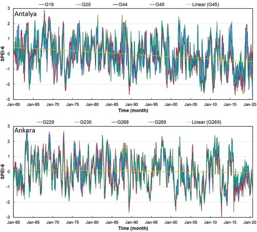
To obtain SPEI timeseries for Antalya and Ankara (see Fig. 1), the global SPEI database (https://spei.csic.es/index.html), which provides long-term SPEI series at a spatial resolution of 1.0° (~100 km), was used. This online database provides 1- to 48-month time scales of SPEI time series for the whole world. As shown in Fig. 1, the data from four grid points within the provinces (the closest points to the cities: G19, G20, G44, and G45 for Antalya and G229, G230, G268, and G269 for Ankara) were retrieved to accomplish the analysis. Figure 2 depicts the SPEI-6 time series of the grid points over the period 1960 to 2020. Overall, a decreasing trend is seen in both regions, with a steeper slope at Antalya. In the first two decades of the period, the SPEI values in Antalya plunged several times to a low of −2.0 or less; however, Ankara did not witness such extreme dry periods. Both regions experienced an exceptionally dry period in the late 1980s, and the number of dry events has dramatically risen over the most recent two decades.

Figure 1. Location of the selected grid points near the cities of Antalya and Ankara, Turkey

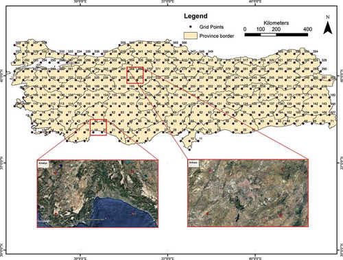
Figure 2. The SPEI-6 timeseries with an example trendline of the selected grid points near the cities of Antalya and Ankara, Turkey

The main statistical features of the series are tabulated in Table 1. The arithmetic mean of the SPEI-6 series of each province was used to represent the meteorological drought variation (target series) at each city. The target series are two vectors having 731 arrays (numerical value) that vary in the range [−2.3, 2.1] and [−2.45, 2.57] for Antalya and Ankara, respectively. Considering the SPEI thresholds suggested by Danandeh Mehr et al. (2020a), we converted the numerical SPEI series at each city to a vector of categorical values including extremely wet (EW; SPEI>1.4), wet (W; 0.5< SPEI<1.4), near normal (NN; −0.5< SPEI<0.5), dry (D; −1.4< SPEI<-0.5), and extremely dry (ED; SPEI<-1.4) arrays. Table 2 demonstrates the absolute count and fractions of the historical drought events at Antalya and Ankara. Naturally, NN is the majority class, and EW followed by ED are the minorities.

Table 1. Geographical and statistical characteristics of the implemented SPEI-6 time series

Station name	Grid point	Latitude (°N)	Longitude (°E)	Min	Mean	Max	Std. dev.	Skewness
Antalya	G18	36.25	29.75	−2.907	−0.065	2.22	1.03	0.026
	G19	36.75	31.75	−3.20	−0.15	2.56	1.08	−0.02
	G43	37.25	39.75	−2.710	−0.14	2.88	1.06	0.07
	G44	37.25	31.75	−3.013	−0.033	2.45	1.02	−0.04
Ankara	G229	39.75	32.75	−2.67	−0.010	2.77	1.029	0.049
	G230	39.75	33.25	−2.66	0.002	2.55	1.03	−0.0004
	G268	40.25	32.75	−2.96	0.022	2.65	1.01	0.034
	G269	40.25	33.25	−2.37	0.039	2.52	0.98	0.03

Table 2. The numbers and fractions of drought events at Antalya and Ankara, Turkey

Station name	Drought class	Absolute count	Fraction
Antalya	NN	261	0.36
	W	179	0.24
	D	191	0.26
	EW	36	0.05
	ED	64	0.09
Ankara	NN	272	0.37
	W	177	0.24
	D	184	0.25
	EW	48	0.07
	ED	50	0.07

3 Methodology

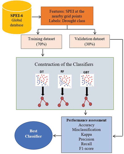
As illustrated in Fig. 3, the modelling process is started by extracting the required data from the global SPEI database. Then, the features are selected, and the label is created through the classification of average SPEI-6 in the study area. Features and the corresponding labels were split into training and holdout validation datasets. The first 70% of the data are used for training the models, and the remaining 30% were utilized as a validation dataset. Inasmuch as we applied DT, RF, and GBT algorithms in this study, different statistical measures, which are explained later in this section, are used to validate the overall and per-class performance of the utilized models.

Figure 3. Flowchart of the methodology used in the present study

3.1 Overview of decision tree

DT is a nonparametric hierarchical supervised data-mining model. Breiman et al. (1984) introduced two types of DT, classification and regression trees, based on the nature of the label data. Both perform in branching sequences consisting of decision nodes (root and leaves) and branches. It is a sort of if–else algorithm that employs recursive partitioning to solve classification and regression problems. In a regression practice, a tree-like classification tree is generated. In the prediction process, the input vectors (features) are split into different branches. Each subset exemplifies a class of available data in the related attribute (Tufaner and Özbeyaz 2020). Considering internal and leaf nodes, each decision node is applied on input variables, and the result is divided into branches. Finally, a leaf node is created where the predicted value is reached in view of a given level of confidence. A multibranch tree is the outcome of this process, which could be used to produce new outputs for new input variables. For more details about the theory and induction of DT, the reader is referred to Quinlan (1986).

3.2 Overview of random forest

In the construction of each DT (single DT), the model may be susceptible to overfitting. Also, input data may involve noise, and thus, a small change in training pattern may cause important impacts on the tree outcome. To overcome these disadvantages, an RF algorithm can be implemented. It is an ensemble DT, i.e. a set of multiple trees, like a forest, in which the outcome is created by averaging the results of its DTs. The RF algorithm consists of two steps: (i) including an arbitrary selection of samples and creating DTs (or estimators) from the bootstrapped dataset; and (ii) performing inference by aggregating predictions of the DTs (Breiman 2001). More information and details about the RF applications in environmental science and water engineering can be found in Tyralis et al. (2019).

3.3 Gradient boosted tree

GBT (Friedman 2001) is a nonlinear ML technique that improves the accuracy of prediction by averaging the weak variables instead of finding a single accurate variable. This method uses iterative techniques to reduce bias and gradually improve estimations. At each step, a new variable is added while the first variable tries to reduce the loss function optimally. The next input variables are fitted to the residuals and shape the DT series from the group of weak prediction classification tree models. Using $x_i$as the single input and $y_i$ as the label with m samples (i = 1, 2, …, m), Danandeh Mehr (2020) described the step-by-step method of GBT as outlined below (Fig. 4):

Figure 4. Step-by-step solution for GBT

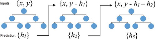
Step 1: A first DT model is used for the samples, which have $h_1$ as their output.

Step 2: The label of the error of the first tree (i.e. $y_i-h_1$) is considered the cost function, and the second DT model is generated.

Step 3: Step 2 is repeated considering the error of the previous tree as a target until the final error reaches the optimum range. Thus, each new tree is corrected based on the previous tree’s error. The final answer is the sum of the new trees which are generated from entire solution.

3.4 Performance evaluation metrics

The performance and accuracy of the new models were assessed using several statistics: overall accuracy (AC), kappa (KA), classification error (CE), class precision (CP), class recall (CR), and F1 score. The AC (Equation 1(1) $AC=\frac{\mathrm{T}\mathrm{P}+\mathrm{T}\mathrm{N}}{m}\times 100$(1) ) is the relative number of properly classified samples. The kappa (Equation 2(2) $KA=\frac{{\mathrm{O}}_{AG}+{\mathrm{E}}_{AG}}{1-{\mathrm{E}}_{AG}}$(2) ) is a chance-adjusted measure of agreement between two observers. The metric adjusts true classifications by removing those correctly classified by chance. The CE (Equation 3(3) $CE=100-\mathrm{A}\mathrm{C}$(3) ) is the overall rate of misclassification, with a value of 0.0 for a perfect model. The CP (Equation 4(4) $CR=\frac{TP}{Tp+FN}$(4) ), also called positive predictive value, is the fraction of relevant examples among the retrieved examples. The CR (Equation 5(5) $CP=\frac{\mathrm{T}\mathrm{P}}{Tp+FP}$(5) ), also called sensitivity, is the fraction of the true samples that were identified correctly. The F1 (Equation 6(6) $F1=\frac{TP}{TP+\frac{1}{2}\left(Fp+FN\right)}$(6) ) is the harmonic mean of precision and recall that conveys the balance between them.

(1) $AC=\frac{\mathrm{T}\mathrm{P}+\mathrm{T}\mathrm{N}}{m}\times 100$(1)

(2) $KA=\frac{{\mathrm{O}}_{AG}+{\mathrm{E}}_{AG}}{1-{\mathrm{E}}_{AG}}$(2)

(3) $CE=100-\mathrm{A}\mathrm{C}$(3)

(4) $CR=\frac{TP}{Tp+FN}$(4)

(5) $CP=\frac{\mathrm{T}\mathrm{P}}{Tp+FP}$(5)

(6) $F1=\frac{TP}{TP+\frac{1}{2}\left(Fp+FN\right)}$(6)

where TP (true positive) and TN (true negative) are the number of correctly labelled events, FN (false negative) and FP (false positive) are the events identified incorrectly, and m is the total sample number. The ${\mathrm{O}}_{AG}$ and ${\mathrm{E}}_{AG}$ are observed and expected agreements, respectively (see Byrt et al. 1993).

4 Results

In the present study, the SPEI-6 indices in Antalya and Ankara cities are classified and predicted over lead times of 1 and 3 months, which are beneficial for early drought warning and short-term decision making. The proposed GBT and benchmarks are tree-based classification-prediction models generated based on the spatiotemporal rules between the lagged SPEI-6 timeseries of the nearby grid points (four grid points) and the drought classes at each city. Akin to other ML techniques in the first step, the entire SPEI dataset for each scenario was separated into two subsets for training (the first 70%: January 1960 to July 2002) and validation (the last 30%: August 2002 to November 2020). Then, DT, RF, and GBT algorithms were trained and verified using RapidMiner, an enterprise ML platform (www.rapidminor.com). In all models, the maximum tree depth was set to 10. To classify and predict the holdout attributes using RF and GBT, their parameters were slightly changed to achieve their optimum values. The maximum number of trees was limited to 100 so that the models were not overfitted.

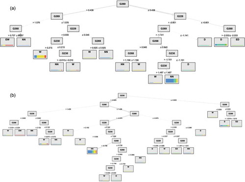
Figures 5 and 6 illustrate the DT models evolved for 1- and 3-month-ahead drought prediction in Antalya and Ankara, respectively. In Antalya, the essential variable to split on is G20. Because the trees are shaped through recursive partitioning, G20 followed by G19 (i.e. points in lower latitudes) are the dominant inputs that bubbled at the top of the tree. This implies sea breezes in the Mediterranean coastal area characterize the meteorological drought condition in Antalya. According to Fig. 5, drought events were fragmented regarding the threshold of −0.75 and +0.77 for 1- and 3-month-ahead prediction scenarios, respectively. In Ankara (see Fig. 6), the SPEI-6 values at the point G269 and G230 (eastern longitudes) are the most essential variables for 1- and 3-month-ahead drought prediction, respectively.

Figure 5. The DT model evolved for (a) 1-month-ahead and (b) 3-month-ahead drought prediction in Antalya, Turkey

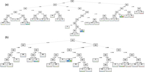
Figure 6. The DT model evolved for (a) 1-month-ahead and (b) 3-month-ahead drought prediction in Ankara, Turkey

The confusion matrices of the evolved DT, RF, and GBT models in the training period are presented in Tables 3 and Tables 4. The associated tables for the validation period are available online (see Supplementary material, Tables S1 and S2). The columns present the ground truth, whereas each row displays a predicted drought event. The number of events, m, given in the captions, helps the reader to recalculate all the performance criteria described in Section 3.4. The tables also include CR and CP measures for each class. In general, the models demonstrate higher class performance in the 1-month-ahead prediction scenario. This may be due to the higher cross-correlation value between the target SPEI series and the first lag of predictors compared to those of the third lag. The cross-correlogram plots (not given in this paper) between the predictors and the associated target series at each city support this conclusion. The class recall of NN events (majority classes) is significantly higher than the other classes, which is mainly due to the greater fraction of this class (see Table 2).

Table 3. Confusion matrix of the models developed for Antalya, Turkey, in the training period (m = 511)

Scenario	Model	True Predicted	NN	W	D	EW	ED	Class precision (%)
1 month ahead	DT	NN	162	34	34	1	0	70.13
		W	25	96	5	13	0	69.06
		D	20	3	69	0	10	67.65
		EW	1	5	0	20	0	76.92
		ED	0	0	2	0	11	84.62
		Class recall (%)	77.88	69.57	62.73	58.82	52.38
	RF	NN	169	34	33	1	0	71.31
		W	20	98	3	18	0	70.50
		D	18	4	73	0	9	70.19
		EW	1	2	0	15	0	83.33
		ED	0	0	1	0	12	92.31
		Class recall (%)	81.25	71.01	66.36	44.12	57.14
	GBT	NN	172	23	20	2	1	78.90
		W	19	103	3	13	0	74.64
		D	15	8	83	0	4	75.45
		EW	1	4	0	19	0	79.17
		ED	1	0	4	0	16	76.19
		Class recall (%)	82.69	74.64	75.45	55.88	76.19
3 months ahead	DT	NN	159	68	52	11	5	53.90
		W	34	66	8	13	2	53.66
		D	12	4	50	1	10	64.94
		EW	1	1	0	9	0	81.82
		ED	0	0	1	0	4	80.00
		Class Recall (%)	77.18	47.48	45.05	26.47	19.05
	RF	NN	32	26	35	2	13	29.63
		W	9	8	11	0	1	27.59
		D	11	5	28	0	26	40.00
		EW	0	0	0	0	0	0.00
		ED	1	0	6	0	3	30.00
		Class Recall (%)	60.38	20.51	35.00	0.00	6.98
	GBT	NN	172	27	18	11	5	73.82
		W	15	102	5	11	2	75.56
		D	17	9	81	0	5	72.32
		EW	1	1	2	12	0	75.00
		ED	1	0	5	0	9	60.00
		Class Recall (%)	83.50	73.38	72.97	35.29	42.86

Table 4. Confusion matrix of the models developed for Ankara, Turkey, in the training period (m = 511)

Scenario	Model	True Predicted	NN	W	D	EW	ED	Class precision (%)
1 month ahead	DT	NN	160	30	42	2	3	67.51
		W	30	101	3	18	0	66.45
		D	10	4	65	0	11	72.22
		EW	2	7	0	17	0	65.38
		ED	0	0	0	0	6	100.00
		Class recall (%)	79.21	71.13	59.09	45.95	30.00	–
	RF	NN	155	28	35	2	2	69.82
		W	29	106	2	17	0	68.83
		D	17	4	71	0	9	70.30
		EW	1	4	0	18	0	78.26
		ED	0	0	2	0	9	81.82
		Class recall (%)	76.73	74.65	64.55	48.65	45.00	–
	GBT	NN	182	18	15	1	4	82.73
		W	10	118	2	13	0	82.52
		D	9	4	91	0	4	84.26
		EW	1	2	0	23	0	88.46
		ED	0	0	2	0	12	85.71
		Class recall (%)	90.10	83.10	82.73	62.16	60.00	–
3 months ahead	DT	NN	171	89	52	21	7	53.90
		W	10	42	5	8	0	53.66
		D	20	12	52	3	9	64.94
		EW	0	0	0	5	0	81.82
		ED	0	0	1	0	4	80.00
		Class recall (%)	85.07	29.37	47.27	13.51	20.00	–
	RF	NN	179	80	54	17	10	52.65
		W	7	53	6	12	0	67.95
		D	15	10	50	3	8	58.14
		EW	0	0	1	5	0	100.00
		ED	0	0	0	0	2	100.00
		Class recall (%)	89.05	37.06	45.45	13.51	10.00	–
	GBT	NN	170	29	32	14	5	67.73
		W	16	106	11	3	2	76.81
		D	11	5	64	2	5	73.56
		EW	4	1	2	18	0	72.00
		ED	0	2	1	0	7	70.00
		Class recall (%)	84.58	74.13	58.18	48.65	42.86	–

The performance results of the evolved DT, RF, and GBT models are tabulated in Table 5. The table shows that the highest classification accuracy belongs to the GBT model, followed by RF. In both cities, the misclassification rate of GBT during the training period is less than 30%, approximately 2 times better than that of DT. According to KA statistics in the training period, which tolerates randomly classified events, the GBT outperforms DT significantly. It is also superior to RF, particularly in Ankara. Regarding the CE values in the validation period, DT was found to be an inappropriate model for generalization goal at 3-month-ahead prediction scenario (63% for Antalya and 61% for Ankara). Following Landis and Koch (1977) and Danandeh Mehr et al. (2020a), the evolved DT, RF, and GBT are respectively considered fair, moderate, and largely satisfactory models for both 1- and 3-month-ahead prediction scenarios in this study.

Table 5. Performance results of the DT, RF, and GBT models in the training and validation periods

Location	Model	Scenario	Training			Validation
			AC (%)	KA	CE (%)	AC (%)	KA	CE (%)
Antalya	DT	1 month ahead	70.1	0.57	29.9	65.7	0.52	34.3
		3 months ahead	56.3	0.35	43.7	36.9	0.14	63.1
	RF	1 month ahead	71.8	0.59	28.2	67.1	0.55	32.9
		3 months ahead	60.3	0.40	39.7	56.2	0.37	43.8
	GBT	1 month ahead	76.9	0.67	23.1	76.7	0.68	23.3
		3 months ahead	73.6	0.62	26.4	67.7	0.55	32.3
Ankara	DT	1 month ahead	68.3	0.542	31.7	50.7	0.32	49.3
		3 months ahead	53.6	0.30	46.4	38.7	0.12	61.3
	RF	1 month ahead	70.2	0.57	29.8	53.9	0.36	46.1
		3 months ahead	56.6	0.34	43.4	41.9	0.16	58.1
	GBT	1 month ahead	83.4	0.76	16.6	54.4	0.37	45.6
		3 months ahead	71.6	0.57	28.5	57.1	0.39	42.9

5 Discussion

The results obtained for Antalya and Ankara are discussed in this section in terms of the per-class performance of the models. Figure 7 presents the number of ground truth (observed) and predicted classes in the training period. It exposes the unbalanced distribution of events in each class that unsurprisingly reveals the complexity of the stochastic problem at hand. Naturally, more than half of the observed samples are categorized as NN. In both Antalya and Ankara, the number of wet events is significantly higher than the number of dry events. This finding agrees with the results of Hesami Afshar et al. (2016), who assessed the SPI series of Ankara province and reported a total of 256 (392) dry (wet) months over the period 1960–2014. Similarly, Bacanlı and Akşan (2019) analysed the SPEI-6 series of Antalya and showed that the relative frequency of EW and ED events stood at 7.19% and 1.15%, respectively, during the time period 1970–2018.

Figure 7. The observed and classified drought events in 1-month-ahead (top panels) and 3-month-ahead (bottom panels) prediction scenarios

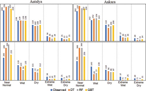
Our results also show that both provinces have the same dry events; however, Antalya experienced slightly more extreme dry/wet events than Ankara during the training period. In both scenarios and cities, the results showed that the NN condition has been overclassified by all the models, but GBT is still superior to its counterparts. Despite higher class precision of the GBT at Antalya, dry events were better classified by DT at Ankara in 3-month-ahead prediction scenario. All the models exhibited similar performance for the classification of the wet events at Antalya. They all underestimate extreme events. The GBT exhibited perfect precision in ED classification at Antalya and outperformed RF and DT in Ankara, which guarantees its superiority for drought classification in the present study. This could be attributed to less information loss in the GBT in comparison to its counterparts.

To further examine the overall performance of the proposed GBT model, Fig. 8 compares the per-class F1 score of this model at Antalya and Ankara in the training period. The associated CP and CR values together with the models’ F1 scores in both training and validation periods are available online (see Supplementary material, Table S3). The figure shows that the new classifier achieves F1 scores of 81% and 86% when predicting NN in Antalya and Ankara with the 1-month-ahead strategy, and 78% and 75% F1 score when predicting with the 3-month-ahead strategy.

Figure 8. F1 score of the GBT drought classification and prediction model at Antalya and Ankara, Turkey

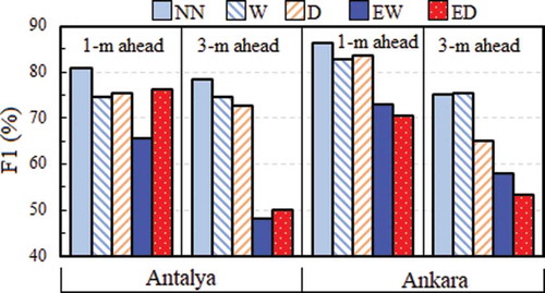
Considering the task of identifying extreme events, a significant drop is observed in the models’ performance, particularly in the 3-month-ahead prediction scenario. This is due to the high-class-imbalance nature of extreme drought events. Obtaining an F1 score of 48%, the most uncertainty is seen in the 3-month-ahead prediction of EW in Antalya, which is much lower than that of Ankara. Such a situation was also observed in the 1-month-ahead prediction scenarios but with F1 scores of 66% and 73% for Antalya and Ankara, respectively. Comparing to the associated values for ED events, one may conclude that EW prediction in Antalya is more challenging.

To support the novelty of the model proposed in the present study, we compared the GBT results with those of the state-of-the-art fuzzy decision tree (FDT) and fuzzy random forest (FRF) classification/forecasting models developed by Danandeh Mehr et al. (2020b) for 1-month-ahead forecasting of SPEI-6 in Antalya. The authors demonstrated FDT (FRF) was a moderately (substantially) satisfactory classifier, achieving a KA statistic of 0.49 (0.61) in the training period and 0.47 (0.65) in the validation period. In the present study, the GBT produced KA statistics of 0.67 and 0.68 in the training and validation periods, respectively. It is, therefore, interpreted as a substantially satisfactory classifier with almost 37% (10%) and 45% (4.6%) superiority over FDT (FRF) in the training and validation periods, respectively.

6 Conclusion

Drought event prediction using classification techniques is a difficult task due to the naturally uneven distribution of drought classes, typically with the majority being near normal and the minority being extreme wet/dry conditions. Many previous studies used station-based historical data to model drought indices from a temporal point of view. In this study, a new robust classifier, called GBT, was employed for spatiotemporal SPEI-6 classification–prediction in Antalya and Ankara using a global SPEI database. The database employs multiple satellite- and model-based meteorological datasets, which provides SPEI at multiple time scales for the entire world. The efficiency of the proposed model was evaluated in terms of AC, KA, CE, PC, RC, and F1 score statistics. Moreover, the GBT performance was compared with the benchmark DT and RF classifiers. The findings revealed that GBT can handle the unbalanced label vector with superiority over RF and DT specifically in the prediction of ED events. Regardless of the highly nonlinear pattern of SPEI-6, the overall training accuracy was about 77% (83%) and 74% (72%) in 1- and 3-month-ahead scenarios in Antalya (Ankara), respectively. The KA values of 0.67 and 0.76 indicated the GBT is a substantially acceptable classifier for 1-month-ahead SPEI-6 classification in the cities. The result measured in terms of F1 score indicated that flood (extreme wet spells) prediction in Antalya is more challenging task than in Ankara.

This study was restricted to 1- and 3-month-ahead classification of a single SPEI time scale (i.e. SPEI-6). Furthermore, parameters of the evolved models were handled using trial and error. Future work using this approach should employ a larger range of SPEI time scales and longer forecasting horizons. A more accurate prediction could be achieved by investigating the effect of parameter tuning using metaheuristic optimization algorithms. To consider the simplicity of the model, we limited this study to the use of only the first lag of the predictors. An investigation on the effect of simultaneous use of several lags of input vectors could also be considered in future. We are primarily interested in SPEI prediction in ungauged catchments. Therefore, the study was limited to the existing global SPEI database such that the accuracy of the results could vary with respect to the database resolution in different latitudes. The higher the resolution, the more truthful the predictions.

Using GBT and exogenous inputs, such as large-scale climate indices or local hydrometeorological variables, a new SPEI prediction/classification model could be developed. An exogenous model may provide additional information about drought, but it would be more complex than the model presented in this study. Moreover, the global SPEI database utilized here has a relatively coarse grid resolution, which may not be a perfect repository to represent drought conditions at a local scale.

Acknowledgements

The authors appreciate the two anonymous reviewers as well as Dr Hristos Tyralis (Associate Editor) for their constructive comments on the initial versions of this paper.

Disclosure statement

No potential conflict of interest was reported by the authors.

Supplementary material

Supplemental data for this article can be accessed here

References

- Bacanlı, Ü.G. and Akşan, G.N., 2019. Drought analysis in Mediterranean region. Pamukkale University Journal of Engineering Sciences, 25 (6), 665–671. doi:https://doi.org/10.5505/pajes.2019.64507
- Baronetti, A., et al., 2020. A weekly spatio-temporal distribution of drought events over the Po Plain (North Italy) in the last five decades. International Journal of Climatology, 40 (10), 4463–4476. doi:https://doi.org/10.1002/joc.6467
- Breiman, L., et al., 1984. Classification and regression trees. Belmont, CA: CRC press.
- Breiman, L., 2001. Random forests. Machine Learning, 45 (1), 5–32. doi:https://doi.org/10.1023/A:1010933404324
- Bulut, B. and Yılmaz, M.T., 2016. Analysis of the 2007 and 2013 droughts in Turkey by NOAH hydrological model. Teknik Dergi, 27 (4), 7619–7634.
- Byrt, T., Bishop, J., and Carlin, J.B., 1993. Bias, prevalence and kappa. Journal of Clinical Epidemiology, 46 (5), 423–429. doi:https://doi.org/10.1016/0895-4356(93)90018-V
- Crausbay, S.D., et al., 2017. Defining ecological drought for the twenty-first century. Bulletin of the American Meteorological Society, 98 (12), 2543–2550. doi:https://doi.org/10.1175/BAMS-D-16-0292.1
- Dabanlı, İ., Mishra, A.K., and Şen, Z., 2017. Long-term spatio-temporal drought variability in Turkey. Journal of Hydrology, 552, 779–792. doi:https://doi.org/10.1016/j.jhydrol.2017.07.038
- Danandeh Mehr, A., 2020. Seasonal rainfall hindcasting using ensemble multi-stage genetic programming. Theoretical and Applied Climatology, 143 (1–2), 461–472. doi:https://doi.org/10.1007/s00704-020-03438-3
- Danandeh Mehr, A., et al., 2020a. Climate change impacts on meteorological drought using SPI and SPEI: case study of Ankara, Turkey. Hydrological Sciences Journal, 65 (2), 254–268. doi:https://doi.org/10.1080/02626667.2019.1691218
- Danandeh Mehr, A., et al., 2020b. A novel fuzzy random forest model for meteorological drought classification and prediction in ungauged catchments. Pure and Applied Geophysics, 177 (12), 5993–6006. doi:https://doi.org/10.1007/s00024-020-02609-7
- Danandeh Mehr, A., 2021. Drought classification using gradient boosting decision tree. Acta Geophysica, 69, 909–918. doi:https://doi.org/10.1007/s11600-021-00584-8
- Danandeh Mehr, A. and Vaheddoost, B., 2020. Identification of the trends associated with the SPI and SPEI indices across Ankara, Turkey. Theoretical and Applied Climatology, 139(3), 1531–1542. doi:https://doi.org/10.1007/s00704-019-03071-9
- Dikshit, A., Pradhan, B., and Alamri, A.M., 2020. Short-term spatio-temporal drought forecasting using random forests model at New South Wales, Australia. Applied Sciences, 10 (12), 4254. doi:https://doi.org/10.3390/app10124254
- Dikshit, A., Pradhan, B., and Alamri, A.M., 2021. Long lead time drought forecasting using lagged climate variables and a stacked long short-term memory model. Science of the Total Environment, 755, 142638. Elsevier B.V. doi:https://doi.org/10.1016/j.scitotenv.2020.142638
- Friedman, J.H., 2001. Greedy function approximation: a gradient boosting machine. The Annals of Statistics, 29(5), 1189–1232. The Institute of Mathematical Statistics. doi:https://doi.org/10.1214/aos/1013203451
- Fung, K.F., et al., 2020. Drought forecasting: a review of modelling approaches 2007–2017. Journal of Water and Climate Change, 11 (3), 771–799. doi:https://doi.org/10.2166/wcc.2019.236
- Fung, K.F., Huang, Y.F., and Koo, C.H., 2019. Coupling fuzzy–SVR and boosting–SVR models with wavelet decomposition for meteorological drought prediction. Environmental Earth Sciences, 78 (24). Springer Berlin Heidelberg. doi:https://doi.org/10.1007/s12665-019-8700-7
- Hesami Afshar, M., Sorman, A.U., and Yilmaz, M.T., 2016. Conditional copula-based spatial–temporal drought characteristics analysis—a case study over Turkey. Water, 8 (10), 426. doi:https://doi.org/10.3390/w8100426
- Keyantash, J. and Dracup, J., 2002. The quantification of drought: an evaluation of drought indices. Bulletin of the American Meteorological Society, 83 (8), 1167–1180. doi:https://doi.org/10.1175/1520-0477-83.8.1167
- Khan, N., et al., 2020. Prediction of droughts over Pakistan using machine learning algorithms. Advances in Water Resources, 139, 103562. doi:https://doi.org/10.1016/j.advwatres.2020.103562
- Landis, J.R. and Koch, G.G., 1977. An application of hierarchical kappa-type statistics in the assessment of majority agreement among multiple observers. Biometrics, 33 (2), 363–374. doi:https://doi.org/10.2307/2529786
- Mckee, T.B., Doesken, N.J., and Kleist, J., 1993. The relationship of drought frequency and duration to time scales. In: Proceedings of the eighth Conference on Applied Climatology. American Meteorological Society. Boston, 179–184.
- Mehdizadeh, S., et al., 2020. Drought modeling using classic time series and hybrid wavelet-gene expression programming models. Journal of Hydrology, 587, 125017. doi:https://doi.org/10.1016/j.jhydrol.2020.125017
- Poornima, S. and Pushpalatha, M., 2019. Drought prediction based on SPI and SPEI with varying timescales using LSTM recurrent neural network. Soft Computing, 23 (18), 8399–8412. doi:https://doi.org/10.1007/s00500-019-04120-1
- Quinlan, J.R., 1986. Induction of decision trees. Machine Learning, 1 (1), 81–106. doi:https://doi.org/10.1007/BF00116251
- Tramblay, Y., et al., 2020. Challenges for drought assessment in the Mediterranean region under future climate scenarios. Earth-Science Reviews, 210 (September), 103348. Elsevier. doi:https://doi.org/10.1016/j.earscirev.2020.103348
- Tufaner, F. and Özbeyaz, A., 2020. Estimation and easy calculation of the palmer drought severity Index from the meteorological data by using the advanced machine learning algorithms. Environmental Monitoring and Assessment, 192 (9). Environmental Monitoring and Assessment. doi:https://doi.org/10.1007/s10661-020-08539-0
- Tyralis, H., Papacharalampous, G., and Langousis, A., 2019. A brief review of random forests for water scientists and practitioners and their recent history in water resources. Water, 11 (5), 910. doi:https://doi.org/10.3390/w11050910
- Van Loon, A.F., 2015. Hydrological drought explained. Wiley Interdisciplinary Reviews: Water, 2 (4), 359–392. doi:https://doi.org/10.1002/wat2.1085
- Vicente-Serrano, S.M., Beguería, S., and López-Moreno, J.I., 2010. A multiscalar drought index sensitive to global warming: the standardized precipitation evapotranspiration index. Journal of Climate, 23 (7), 1696–1718. doi:https://doi.org/10.1175/2009JCLI2909.1
- Yılmaz, E. and Çiçek, İ., 2018. Detailed Köppen-Geiger climate regions of Turkey Türkiye’nin detaylandırılmış Köppen-Geiger iklim bölgeleri. Journal of Human Sciences, 15 (1), 225–242. doi:https://doi.org/10.14687/jhs.v15i1.5040
- Zhang, Y., et al., 2020. Comparison of the ability of ARIMA, WNN and SVM models for drought forecasting in the Sanjiang Plain, China. Natural Resources Research, 29 (2), 1447–1464. doi:https://doi.org/10.1007/s11053-019-09512-6