A new method for assessing hydrologic alterations based on the discharge hydrograph

ABSTRACT

Ecosurplus (ES) and ecodeficit (ED) based on flow duration curves have been used to assess hydrological alterations in contemporary research, but there are associated limitations. In this study a new method based on the discharge hydrograph is presented. The 12 monthly ESs and 12 monthly EDs constitute a new suite of indicators. Two types of equations are presented to calculate the degree of change in the ESs and EDs. A framework is proposed for classifying the risk of monthly EDs into four levels. Results show that inconsistencies among the eco-flows on different time scales ceased to exist. The second equation type showed a stronger performance in measuring the changes of monthly eco-flows. The risk graph intuitively demonstrates the risk levels of each month over past decades. The 24 indicators did not have strong correlations. This study is useful for water resource management considering the variations resulting from reservoir regulations.

KEYWORDS:

• hydrological alterations
• ecosurplus
• ecodeficit
• discharge hydrograph
• risk assessment

Editor A. Fiori Associate editor S. Lyon

1 Introduction

Building reservoirs on rivers can provide electricity for economic development and water for irrigation; however, it can alter the hydrological regimes of rivers, especially downstream. The altered hydrological regimes may have adverse impacts on river ecosystems, as a natural flow regime before damming is considered to be the best condition to sustain aquatic ecosystems (Arthington et al. 2006). Multiple metrics have been proposed in previous studies, including the most popular indicators of hydrological alteration (IHA), which incorporate 33 indicators (Richter et al. 1996). However, statistical redundancy exists among these 33 indicators (Olden and Poff 2003). Therefore, research has committed to overcoming the redundant information, and developing new statistically independent metrics. Eco-flows, including ecosurplus (ES) and ecodeficit (ED) proposed by Vogel et al. (2007), are an example of these metrics. Gao et al. (2009) concluded that ES and ED provide a good overall representation of the degree of alteration of hydrological regimes.

Eco-flows are calculated based on the flow duration curve (FDC) (Vogel and Fennessey 1994, 1995, Ghotbi et al. 2020). An annual FDC is obtained by sorting the daily discharges in a year from largest to smallest. Using annual FDCs before damming, the 25^th percentile FDC and 75^th percentile FDC can be calculated and taken as the lower and upper limits of the protection target (Gao et al. 2012, Wang et al. 2017). For each annual FDC, the area above the 75^th percentile FDC represents the excess of runoff relative to the upper limit during that year. The annual ES equals the area divided by the annual mean discharge. The area below the 25^th percentile FDC represents the shortage of runoff relative to the lower limit during that year. The annual ED equals the area divided by the annual mean discharge (Wang et al. 2017). Similarly, the monthly and seasonal eco-flows are obtained by using the monthly and seasonal FDCs, respectively. Eco-flows have been used to assess hydrological alterations by an increasing number of studies (Gao et al. 2012, 2018, Gu et al. 2016, Zhang et al. 2015, 2018, Wang et al. 2017, Lu et al. 2018, Ali et al. 2019, Sharma et al. 2019, Zhou et al. 2019). However, this method is not as well studied as the most popular IHA (Richter et al. 1996) because four significant limitations currently impede its application.

The first limitation is the inconsistent conclusions that are reached depending on the time scales. Vogel et al. (2007) stated that annual, seasonal, and monthly FDCs were used to calculate the annual, seasonal, and monthly eco-flows, respectively. However, two problems arose with their results. First, the sum of eco-flows on a short time scale is not equal to those on a long time scale; that is, the sum of three monthly eco-flows does not equal the seasonal eco-flows, and the sum of four seasonal eco-flows does not equal the annual eco-flows. The inequality does not conform to the hydrological terminologies such as monthly, seasonal, and annual runoff. Second, monthly ED or ES may be non-zero while seasonal and/or annual ED or ES may be zero. The contradictory ES or ED on different time scales often confused river managers; therefore the results calculated by FDCs often make it challenging to correctly assess the health status of rivers.

Second, no previous studies have suggested a method for measuring the level of change of these eco-flows after they are impacted. Although many previous studies have reported annual and seasonal eco-flows, only qualitative analyses have been undertaken, and no quantitative equations have been presented to date (Gao et al. 2012, 2018, Zhang et al. 2015, 2018, Wang et al. 2017, Lu et al. 2018). However, in other methods such as IHA, the range of variability approach (RVA) (Richter et al. 1997) and other equations (Shiau and Wu 2007, Chen et al. 2010) have been used to calculate the degree of alteration, which may have contributed towards the wide use of IHA. The lack of equations available to quantitatively measure the degree of change of eco-flows hinders its application.

Third, there is no framework that describes the risk levels corresponding to different values of ES and ED. Such a framework, which could evaluate risk based on eco-flows, would help us better understand the health status of a river, and would significantly improve the usability of eco-flows. Using the IHA as an example, Black et al. (2005) determined the level of river flow regime alterations via the Dundee Hydrological Regime Alteration Method (DHRAM). They classified the regime alterations into five levels: unimpacted, low risk of impact, moderate risk of impact, high risk of impact, and severely impacted. This classification drove the application of IHA. However, no similar frameworks currently exist for assessing hydrological alterations by eco-flows.

Fourth, a lack of sufficient biological data also limits the applications of eco-flows. Developing the aforementioned framework for the eco-flows has two key issues. First, the relevance or direct link of eco-flows to biological health and stream function is currently unknown. More specifically, research on responses of biological health to the alterations of eco-flows is scarce. For example, using long-term monitoring data of the Illinois River fish population, Yang et al. (2008b) developed a quantitative function describing the relationships between some indicators of IHA and the Shannon diversity index. The function can be used to indirectly assess the rivers without requiring observed fish data. Second, the level of alteration expected in order to observe risk to stream biology is unclear; that is, the level of ED or ES that is acceptable/unacceptable is not confirmed. The solutions to these issues require sufficient biological data. However, it is not always easy for researchers to access these data.

These four limitations restrict the usability of eco-flows in assessing hydrological alterations. Therefore, the objectives of this study are as follows: (a) to define a new ES and ED that are not characterized by inconsistencies on different time scales, and develop a suite of eco-flow indicators; (b) to present a way of measuring the degree of changes in ES and ED; (c) to develop a risk assessment framework for the indicators; and (d) to develop a system for assessing hydrological alterations by eco-flows. The proposed method paves the way for future studies to assess the health of river ecosystems, and the results can aid policymakers and managers to design a sustainable ecological regulation strategy of reservoirs to mitigate the negative effects of dams on downstream river ecosystems.

2 Methods

2.1 Monthly eco-flow indicators

The discharge hydrograph (DH) represents a true daily discharge process with no re-ordering. Similar to the 25^th and 75^th percentile FDCs, which are taken as the lower and upper limits of the protection target (Gao et al. 2012, Wang et al. 2017), the two percentiles are also used in the present method. For example, if the daily discharge data span 46 years before damming, for 1 January, the 25^th percentile daily discharge on this day can be counted from the 46 values on this day in each year. The 25^th percentile daily discharges on other days in a year can be similarly obtained. All of the 25^th percentile daily discharges on each day constitute the 25^th percentile DH. Similarly, the 75^th percentile DH are constituted by the 75^th percentile daily discharges on each day. The area between the two DHs is considered to be the adaptive range (Fig. 1(a)).

Figure 1. Definitions of the eco-flows by DH. (a) River management targets (magenta area) are between the 25^th percentile DH (red dashed line) and the 75^th percentile DH (green dashed line). (b) The area (green area) below the 75^th percentile discharge hydrograph (DH) in a month is the maximum ecological water requirement of the month $Max{W}_m$. (c) The area (red area) below the 25^th percentile discharge hydrograph (DH) in a month is the minimum ecological water requirement of the month $Min{W}_m$.

DH is the abbreviations of discharge hydrograph;

MaxW is the abbreviations of maximum ecological water requirement;

MinW is the abbreviations of minimum ecological water requirement

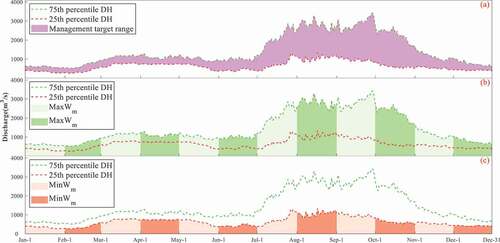
As the ES and ED denote the excess and shortage, respectively, of runoff relative to the protection target during a period, two important variables – the maximum ecological water requirement ($MaxW$) and the minimum ecological water requirement ($MinW$) – are first defined for each month. For example; the area below the 75^th percentile DH from 1 to 31 January, which is a product of daily discharge and time, is defined as January $MaxW$ (Fig. 1(b)), and the area below the 25^th percentile DH from 1 to 31 January is defined as January $MinW$ (Fig. 1(c)). $MaxW$ and $MinW$ of the other months can be calculated accordingly.

For a given annual DH (Fig. 2), the daily discharges exceeding the 75^th percentile DH from 1 to 30 June are shown in Fig. 2 (cyan area). The sum of the area is the surplus runoff in June. Daily discharges below the 25^th percentile DH from 1 to 31 August are also shown in Fig. 2 (yellow area). The sum of the yellow area during this period is the deficient runoff in August. The monthly ES and ED are defined as:

(1) $E{S}_m=\frac{D{\sum }_{i=1}^n\left(Q_i-Q_{i,75\mathrm{\%}}\right)}{Max{W}_m},if{Q}_i>Q_{i,75\mathrm{\%}}$(1)

(2) $E{D}_m=\frac{D{\sum }_{i=1}^n\left(Q_i-Q_{i,25\mathrm{\%}}\right)}{Min{W}_m},if{Q}_i<Q_{i,25\mathrm{\%}}$(2)

Figure 2. Definition of surplus runoff (cyan area) and deficient runoff (yellow area) by DH in a given year

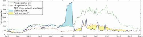
where m denotes the month, m = 1 for January etc.; D = 86,400 s; n is the number of days in each month, n = 31 for January etc.; $Q_{i,75\mathrm{\%}}$ and $Q_{i,25\mathrm{\%}}$ denote the 75^th percentile and 25^th percentile daily discharge, respectively; and $Max{W}_m$ and $Min{W}_m$ are the $MaxW$ and $MinW$ of the mth month, respectively. The numerator of Equation (1)(1) $E{S}_m=\frac{D{\sum }_{i=1}^n\left(Q_i-Q_{i,75\mathrm{\%}}\right)}{Max{W}_m},if{Q}_i>Q_{i,75\mathrm{\%}}$(1) indicates the surplus runoff in a month, and that of Equation (2)(2) $E{D}_m=\frac{D{\sum }_{i=1}^n\left(Q_i-Q_{i,25\mathrm{\%}}\right)}{Min{W}_m},if{Q}_i<Q_{i,25\mathrm{\%}}$(2) is the deficient runoff in a month (Fig. 2). After dividing by $MinW$ and $Min{W}_m$, respectively, $Min{W}_m$ quantifies how much higher the value is than $Max{W}_m$, and $Max{W}_m$ quantifies how much lower the value is compared to $Min{W}_m$. $Min{W}_m$ is non-negative, and $E{D}_m$ is non-positive. A negative value of $E{D}_m$ indicates a lack of water. These different signs aid the ability to distinguish ES from ED and are simple to apply.

In addition to the monthly eco-flows, seasonal eco-flows can be defined as the sum of three monthly values based on the local climate. Annual eco-flows are the sum of 12 monthly values. Therefore, there must be no inconsistencies among eco-flows at different time scales. In this study, the 24 monthly eco-flow indicators (24 MEIs) were adopted to assess hydrological alteration (Table 1). They were divided into two groups: Group 1 included 12 monthly ES values, and Group 2 included 12 monthly ED values.

Table 1. The 24 monthly eco-flow indicators proposed in this study

No.	Group 1	No.	Group 2
1	January ES	1	January ED
2	February ES	2	February ED
3	March ES	3	March ED
4	April ES	4	April ED
5	May ES	5	May ED
6	June ES	6	June ED
7	July ES	7	July ED
8	August ES	8	August ED
9	September ES	9	September ED
10	October ES	10	October ED
11	November ES	11	November ED
12	December ES	12	December ED

ES is the abbreviations of Ecosurplus;

ES is the abbreviations of Ecodeficit

2.2 Degree of change in monthly eco-flows

To investigate the degree of change of each indicator, two types of equations are proposed. The first type is similar to those used for calculating the hydrological alteration of IHA (Yang et al. 2008a; Wang et al. 2015, 2016, Zhang et al. 2015, 2018). Based on Equations (1)(1) $E{S}_m=\frac{D{\sum }_{i=1}^n\left(Q_i-Q_{i,75\mathrm{\%}}\right)}{Max{W}_m},if{Q}_i>Q_{i,75\mathrm{\%}}$(1) and (2(2) $E{D}_m=\frac{D{\sum }_{i=1}^n\left(Q_i-Q_{i,25\mathrm{\%}}\right)}{Min{W}_m},if{Q}_i<Q_{i,25\mathrm{\%}}$(2) ), the monthly ES and ED values are zero if the corresponding DH is in the target range. The first type of equation is as follows:

(3) $D_{ES}^m=\frac{N_{obs,ES}^m-N_{exp,ES}^m}{N_{exp,ES}^m}$(3)

(4) $N_{exp,ES}^m=\frac{N_{pre,ES}^m}{N_{pre}}{N}_{post}$(4)

(5) $D_{ED}^m=\frac{N_{obs,ED}^m-N_{exp,ED}^m}{N_{exp,ED}^m}$(5)

(6) $N_{exp,ED}^m=\frac{N_{pre,ED}^m}{N_{pre}}{N}_{post}$(6)

where $D_{ES}^m$ denotes the degree of change in the mth monthly ES; $N_{obs,ES}^m$ is the number of years in which the mth monthly ES is zero in the post-impact years; $N_{exp,ES}^m$is the number of years in which the mth monthly ES is expected to be zero in the post-impact years; $N_{pre}$ and $N_{post}$are the number of years in the pre- and post-impact time series, respectively; and $N_{pre,ES}^m$ is the number of years in which the mth monthly ES is zero in the pre-impact years. Equation (4)(4) $N_{exp,ES}^m=\frac{N_{pre,ES}^m}{N_{pre}}{N}_{post}$(4) indicates that $N_{exp,ES}^m$ is expected based on the frequency of zero monthly ES in the pre-impact years. $D_{ED}^m$, $N_{obs,ED}^m$, and $N_{exp,ED}^m$ have the same meaning as the equivalent notation for ES but represent ED instead. Further, the first type represents a change in the frequency at which the zero monthly eco-flows occurred.

In contrast, the second type of equations focuses on the years in which the monthly ES or ED is not zero. The second type is as follows:

(7) $D_{ES}^m=\hspace{0.17em}\frac{\sum _{i=1}^{N_{post}}E{S}_{obs,i}^m-TE{S}_{exp}^m}{TE{S}_{exp}^m}$(7)

(8) $TE{S}_{exp}^m=\frac{N_{post}}{N_{pre}}{\sum }_{i=1}^{N_{pre}}E{S}_{obs,i}^m$(8)

(9) $D_{ED}^m=\hspace{0.17em}\frac{\sum _{i=1}^{N_{post}}E{D}_{obs,i}^m-TE{D}_{exp}^m}{TE{D}_{exp}^m}\hspace{0.17em}$(9)

(10) $TE{D}_{exp}^m=\frac{N_{post}}{N_{pre}}{\sum }_{i=1}^{N_{pre}}E{D}_{obs,i}^m$(10)

where $E{S}_{obs,i}^m$ is the mth monthly ES of the ith year; ${\sum }_{i=1}^{N_{post}}E{S}_{obs,i}^m$ denotes the sum of the mth monthly ES in the post-impact years, that is, the sum of the non-zero mth monthly ES after being disturbed; $TE{S}_{exp}^m$ is the expected total of the mth monthly ES in the post-impact years, and it is expected based on that in the pre-impact years; $TE{S}_{exp}^m$ denotes the sum of the mth monthly ES in the pre-impact years, that is, the sum of the non-zero mth monthly ES before being disturbed; $E{D}_{obs,i}^m$ and $E{D}_{obs,i}^m$ have the same meaning as those of ES but represent ED instead.

As noted above, the second type considers only the non-zero monthly ES or ED. Equation (7)(7) $D_{ES}^m=\hspace{0.17em}\frac{\sum _{i=1}^{N_{post}}E{S}_{obs,i}^m-TE{S}_{exp}^m}{TE{S}_{exp}^m}$(7) indicates how much the cumulative mth monthly ES has changed. A positive $D_{ES}^m$ indicates the monthly runoff was more than what was expected, implying there was more monthly runoff exceeding the 75^th percentile DH. A negative $D_{ES}^m$ indicates that monthly runoff was less than expected, implying that less monthly runoff exceeding the 75^th percentile DH occurred. Conversely, a positive $D_{ED}^m$ indicates that the cumulative mth monthly ED was greater than expected, implying that more monthly runoff below the 25^th percentile DH occurred, which is an adverse situation for rivers. A negative $D_{ED}^m$ indicates that monthly runoff was less than expected, implying that less monthly runoff below the 25^th percentile DH occurred (which is a beneficial situation). The results from the two equation types were compared using the observed daily discharge time series, and the type capable of exhibiting optimal performance was determined.

2.3 Risk level of monthly ED

The degree of change provides information on how much the monthly eco-flows changed; however, individuals managing the river still had no intuitive understanding of the level of monthly ES and ED. Gao et al. (2009) highlighted that the ED and ES do not include the risk level and suggested establishing a system to classify what level of ED or ES is acceptable/unacceptable. Further, there has been no published progress on this topic since 2009.

In this study, a framework describing the risk level of monthly ED is proposed. In this framework, two monthly EDs of each month were first calculated by using the 10^th percentile DH and 20^th percentile DH based on Equation (2(2) $E{D}_m=\frac{D{\sum }_{i=1}^n\left(Q_i-Q_{i,25\mathrm{\%}}\right)}{Min{W}_m},if{Q}_i<Q_{i,25\mathrm{\%}}$(2) ), and taken as the respective threshold values (Table 2). The reasons for selecting the 10^th and 20^th percentiles are detailed in the Discussion section. The daily discharges used in Table 2 are from the following case study. Four risk levels are proposed: no risk, low risk, moderate risk, and high risk (Table 3). For instance, if the January ED in a given year is smaller than that calculated by the 10^th percentile DH (−0.269, Table 2), January has high risk. If it is larger than −0.269 but smaller than −0.070 (Table 2), January has moderate risk. If it is larger than −0.070 but smaller than 0, January has low risk. If it is 0, January has no risk. The corresponding relationships are shown in Table 3.

Table 2. Respective monthly ED values corresponding to the 10^th and 20^th percentile DH

Group 2	10^th DH	20^th DH	Group 2	10^th DH	20^th DH
January ED	−0.268	−0.070	July ED	−0.447	−0.112
February ED	−0.400	−0.083	August ED	−0.402	−0.164
March ED	−0.164	−0.056	September ED	−0.381	−0.105
April ED	−0.134	−0.037	October ED	−0.327	−0.120
May ED	−0.275	−0.063	November ED	−0.435	−0.122
June ED	−0.503	−0.177	December ED	−0.251	−0.064

Table 3. Risk levels according to the monthly ED

Group 2	Risk level
Monthly ED = 0	No risk
20^th percentile DH ≤ Monthly ED < 0	Low risk
10^th percentile DH ≤ Monthly ED < 20^th percentile DH	Moderate risk
Monthly ED < 10^th percentile DH	High risk

Here, the monthly ES is not adopted to describe the risk level. It is important to note that this study focused on the downstream impacts of dam operations. As the main functions of most dams are flood control, power generation and agricultural irrigation, the resultant flow depletion downstream of the dams is the primary concern. However, in other settings, such as highly urbanized or agricultural watersheds, if flow augmentation from urban drool or irrigation return flow is negatively impacting streams, ES and risk should be evaluated. The risk evaluation method in terms of monthly ES requires further study.

3 Case study

The Yellow River is the second longest river in China; it measures 5,464 km in length with a basin area of 752 000 km². Xiaolangdi reservoir has the largest capacity in the river and was completed in December 2001. The reservoir is mainly used to prevent floods and to generate electricity. It has a drainage area of 694 000 km², accounting for 92.3% of the entire basin. The reservoir is located 896 km from the Yellow River Estuary. As a key reservoir, it significantly alters the downstream flow regime.

The Xiaolangdi hydrological station is located 4 km downstream of the dam, and no tributary exists between the dam and the station. The available daily discharge time series at the station spans from 1956 to 2015. The whole time series is subdivided into two subseries: 1956 to 2001 and 2002 to 2015. The period from 1956 to 2001 was the natural status. The 25^th percentile and 75^th percentile DHs were obtained using daily discharge from 1956 to 2001.

4 Results and discussion

4.1 Variation tendency

Using the daily discharge time series from the Xiaolangdi hydrological station, the 24 monthly eco-flow indicators for each year could be obtained using Equations (1)(1) $E{S}_m=\frac{D{\sum }_{i=1}^n\left(Q_i-Q_{i,75\mathrm{\%}}\right)}{Max{W}_m},if{Q}_i>Q_{i,75\mathrm{\%}}$(1) and (2(2) $E{D}_m=\frac{D{\sum }_{i=1}^n\left(Q_i-Q_{i,25\mathrm{\%}}\right)}{Min{W}_m},if{Q}_i<Q_{i,25\mathrm{\%}}$(2) ). Previous studies have often plotted the annual or seasonal ES and ED in each year and attempted to examine their long-term changes (Gao et al. 2012, 2018, Zhang et al. 2015, Wang et al. 2017, Lu et al. 2018). However, it is impossible to determine the variation tendency clearly from such plots, because the eco-flows are sometimes zero. To justify the variation tendency directly, the cumulative monthly ES and ED were plotted in this study (Fig. 3).

Figure 3. Cumulative monthly ES (green lines) and cumulative monthly ED (red lines)

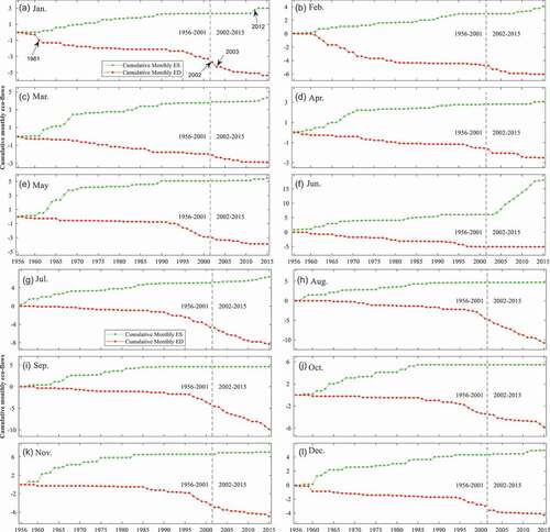
Figure 3 shows that the cumulative monthly ES (green dotted lines) and cumulative monthly ED (red dotted lines) increased at different rates. The endpoint (on the right) of a line segment with a steep gradient corresponds to a year in which the monthly eco-flows were significantly larger than the previous year. The endpoint (on the right) of a horizontal line segment corresponds to a zero monthly ES or ED. Taking January as an example (Fig. 3(a)), the red line segment between 1960 and 1961 is very steep, implying that the absolute January ED in 1961 (−0.681) was much larger than that in 1960 (−0.051). Similar scenarios include the red line segment between 2002 and 2003, and the green line segment between 2011 and 2012.

In addition, the overall gradient of the slope can qualitatively reveal the variation tendency. Using June as an example, the green line increased gradually in the pre-impact years and rapidly in the post-impact years, implying that the June ES became large. Then, the red line shifted from a descending gradient to a plateau, implying that the ED in June changed to zero. Therefore, the ideal situation for ensuring river health is when the red line remains mostly flat, descending occasionally. To investigate their degree of change more accurately, the equations provided in the second sub-section of the Methods were applied.

4.2 Difference between the two types of equations

The two types of equations were used to calculate the degree of change (Table 4). In the first type, a positive degree of change in monthly ES indicates that the number of years with zero monthly ES was greater than expected, which implies that the years with non-zero monthly ES occurred less frequently than before, thus an adverse change in the health of the river can be assumed, labelled “worse” (while opposite conditions are referred to as “better”). A positive degree of change in monthly ED indicates that the number of years with zero monthly ED is greater than expected, which means that the years with non-zero monthly ED occurred less frequently than before, and thus a beneficial change for the health of the river can be assumed, labelled “better” (the opposite conditions are referred to as “worse”). For the second type, the positive and negative degree of change and their corresponding implications are also explained (Table 4).

Table 4. Degree of change and corresponding description according to the two types of equations

24 MEIs	First equation type		Second equation type
	Degree of change (%)	Description	Degree of change (%)	Description
January ES	55.63	Worse	−5.48	Worse
February ES	−8.73	Better	29.48	Better
March ES	17.34	Worse	−48.54	Worse
April ES	87.75	Worse	−69.51	Worse
May ES	82.53	Worse	−74.13	Worse
June ES	−61.34	Better	544.19	Better
July ES	−45.23	Better	−14.29	Worse
August ES	158.16	Worse	−97.76	Worse
September ES	84.00	Worse	−100.00	Worse
October ES	70.85	Worse	−99.60	Worse
November ES	57.71	Worse	−76.97	Worse
December ES	75.23	Worse	−52.40	Worse
January ED	−42.01	Worse	109.41	Worse
February ED	2.67	Better	−8.36	Better
March ED	−17.85	Worse	48.72	Worse
April ED	−13.53	Worse	99.36	Worse
May ED	9.52	Better	10.55	Worse
June ED	131.93	Better	−97.71	Better
July ED	−100.00	Worse	161.26	Worse
August ED	−100.00	Worse	350.36	Worse
September ED	−100.00	Worse	377.25	Worse
October ED	−89.04	Worse	130.43	Worse
November ED	−34.28	Worse	84.73	Worse
December ED	9.52	Better	40.52	Worse

In Table 4, the two types have identical descriptions in most cases except for July ES, May ED, and December ED (the shaded area in Table 4). These three indicators have opposite qualitative descriptions. To investigate which is more accurate, the values of each indicator in the pre-impact years (1956–2001) and post-impact years (2002–2015) were averaged (Table 5). Using the July ES, for example (the shaded area in Table 5), its averaged value in the post-impact years (0.094) was smaller than in the pre-impact years (0.110), implying that the average sufficient runoff in July fell to less than before, an apparent adverse change to the river ecosystem. Therefore, the second type of equation is more accurate. Comparisons of the averaged May ED and December ED in the two periods also validated the reasonability of the second type. The failure of the first type proves that the change in frequency at which the normal monthly flow events occurred is limited in measuring the changes of 24 MEIs.

Table 5. Average monthly eco-flows in the pre-impact (1956–2001) and post-impact (2002–2015) periods

Group 1 (ES)	Pre-impact	Post-impact	Group 2 (ED)	Pre-impact	Post-impact
January	0.051	0.048	January	−0.071	−0.149
February	0.064	0.083	February	−0.103	−0.094
March	0.082	0.042	March	−0.043	−0.064
April	0.061	0.018	April	−0.034	−0.068
May	0.110	0.029	May	−0.063	−0.070
June	0.132	0.854	June	−0.110	−0.003
July	0.110	0.094	July	−0.101	−0.263
August	0.102	0.002	August	−0.099	−0.446
September	0.099	0	September	−0.087	−0.416
October	0.119	0.0004	October	−0.074	−0.171
November	0.143	0.033	November	−0.096	−0.178
December	0.094	0.045	December	−0.065	−0.091

Table 4 demonstrates that the June ES and June ED improved, validating the qualitative judgement discussed in the previous section. The February ES and February ED also improved. The remaining indicators worsened. Therefore, the second type can accurately measure the changes of monthly eco-flows, and is a good supplement to the cumulative monthly eco-flow curves (Fig. 3).

4.3 Risk evaluation

The risk levels of each monthly ED from 1956 to 2015 were evaluated and plotted in a risk graph (Fig. 4). Figure 4 clearly illustrates the risk levels for each month from 1956 to 2015. Overall, no risk instances were more frequently observed in the pre-impact period (1956–2001) compared with the post-impact period (2002–2015). There are three characteristic areas in Fig. 4. The first is the nearly continuous white rectangles of June from 2002 to 2015, which were at low risk previously. The second is the nearly continuous crimson rectangles of July, August, and September after 2001; however, no-risk and low-risk categories dominated prior to 2002. The third is the nearly continuous white rectangles of October and November from 1961 to 1985. Since 1995, they have often transitioned into the moderate risk category and occasionally into the high risk category.

Figure 4. Risk graph of monthly ED from 1956 to 2015

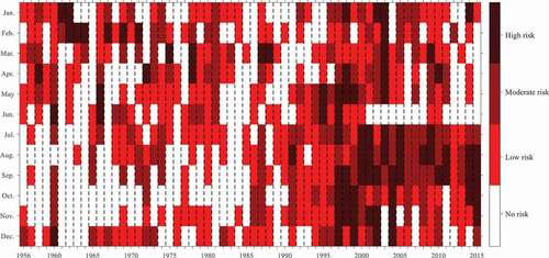
To quantitatively describe the risk graph, the percentages of years exhibiting high and moderate risk levels of monthly ED are shown in Table 6. During the pre-impact period, February and May demonstrated the maximum percentages of high risk levels. This implies that severe droughts occurred more frequently at the end of winter (from December to February) and spring (from March to May), as the dry season includes the winter and spring in the Yellow River Basin. Meanwhile, April and July demonstrated the maximum percentages of moderate risk levels. During the post-impact period, July and August exhibited the maximum percentages of high risk levels. This can be attributed to the function of preventing the flooding of the Xiaolangdi reservoir, as floods generally occur in these two months in the basin. The decrease of the daily discharge in these two months caused an apparent increase of their monthly EDs.

Table 6. The percentage of years for each monthly ED with moderate and high risk

Month	Pre-impact period (1956–2001)		Post-impact period (2002–2015)
	High (%)	Moderate (%)	High (%)	Moderate (%)
January	6.52	19.56	21.42	21.42
February	13.04	17.39	7.14	21.42
March	8.69	19.56	14.28	21.42
April	8.69	21.73	14.28	21.42
May	10.86	15.21	7.14	28.57
June	8.69	13.04	21.42	57.14
July	6.52	21.73	50.0	42.85
August	6.52	15.21	50.0	42.85
September	8.69	19.56	21.42	21.42
October	6.52	17.39	21.42	21.42
November	8.69	10.86	14.28	14.28
December	6.52	19.56	21.42	21.42

The overall risk levels in the pre-impact (1956–2001) and post-impact (2002–2015) periods were evaluated based on their averaged monthly ED (Table 7). In the pre-impact period (1956–2001), nine monthly EDs were categorized as low risk, and only three monthly EDs were moderate risk (January, February, and December). Therefore, low risk was the major risk level. In the post-impact period (2002–2015), one monthly ED was low risk, nine monthly EDs were moderate risk, and two monthly EDs were high risk. Therefore, moderate risk was the main risk level. The comparisons showed that eight monthly EDs rose while four monthly EDs remained unchanged. The August ED and September ED rose from low to high risk directly, which is also reflected by the degree of change (Table 4); they increased by 350.36% and 377.25%, respectively. Overall, the risk levels of 12 monthly EDs increased.

Table 7. Risk levels evaluated by average monthly ED in the pre-impact (1956–2001) and post-impact (2002–2015) periods

Group 2	Pre-impact	Post-impact	Tendency	Group 2	Pre-impact	Post-impact	Tendency
January ED	Moderate	Moderate	→	July ED	Low	Moderate	↑
February ED	Moderate	Moderate	→	August ED	Low	High	↑
March ED	Low	Moderate	↑	September ED	Low	High	↑
April ED	Low	Moderate	↑	October ED	Low	Moderate	↑
May ED	Low	Moderate	↑	November ED	Low	Moderate	↑
June ED	Low	Low	→	December ED	Moderate	Moderate	→

Note: ↑: increasing risk level, ↓: decreasing risk level, →: no change.

4.4 Intercorrelations

Gao et al. (2009) noted that the information redundancy existing in the IHA cannot help river managers make effective decisions. Therefore, developing a set of independent indicators is one of the goals of characterizing hydrological alterations caused by reservoirs. To explore the intercorrelations of the proposed 24 MEIs, Pearson’s r correlation coefficients between each MEI statistics and the remaining 23 MEI statistics were investigated and are shown in Tables 8, 9, and 10. Shading of numbers in these tables indicates that the correlation is significant at α = 0.001.

Table 8. Correlation coefficients among the 12 monthly ES statistics

	January	February	April	March	May	June	July	August	September	October	November
February	0.341
April	0.239	0.311
March	0.253	0.146	0.484
May	0.171	–0.006	0.363	0.718
June	0.103	0.100	–0.126	0.102	0.165
July	–0.051	–0.002	0.076	0.370	0.387	0.167
August	–0.012	–0.082	0.033	0.308	0.293	–0.049	0.628
September	0.071	–0.001	0.191	0.448	0.560	–0.024	0.419	0.619
October	0.004	–0.044	0.153	0.474	0.669	0.050	0.422	0.339	0.616
November	–0.033	0.020	0.018	0.428	0.504	0.104	0.518	0.341	0.318	0.763
December	0.108	–0.002	0.081	0.356	0.497	0.153	0.352	0.132	0.128	0.572	0.754

Table 9. Correlation coefficients among the 12 monthly ED statistics. Shading of numbers indicates that the correlation is significant at α = 0.001

	January	February	April	March	May	June	July	August	September	October	November
February	0.155
April	–0.157	0.261
March	0.034	–0.107	0.336
May	0.167	–0.259	–0.118	0.361
June	–0.037	–0.062	0.011	0.300	0.511
July	0.147	–0.148	–0.112	0.108	0.518	0.299
August	0.026	0.023	–0.024	0.035	0.158	–0.139	0.706
September	0.149	–0.039	–0.097	0.231	0.405	0.167	0.766	0.764
October	0.103	–0.249	–0.080	0.384	0.591	0.246	0.596	0.369	0.737
November	0.068	–0.195	–0.104	0.301	0.495	0.193	0.659	0.549	0.766	0.839
December	–0.017	–0.144	–0.082	0.234	0.297	0.428	0.299	0.146	0.462	0.477	0.492

Table 10. Correlation coefficients between the 12 monthly EDs (first column) and 12 monthly ESs (first row). Shading of numbers indicates that the correlation is significant at α = 0.001

	January	February	April	March	May	June	July	August	September	October	November	December
January	0.191	0.110	0.200	0.138	0.292	0.129	0.274	0.148	0.166	0.174	0.177	0.121
February	–0.140	–0.003	0.302	0.214	0.186	0.124	0.190	0.141	0.153	0.052	0.094	0.161
April	–0.055	–0.464	0.160	0.260	0.289	0.009	0.262	0.188	0.147	0.242	0.252	0.156
March	–0.137	–0.528	0.090	0.387	0.325	0.169	0.236	0.123	0.171	0.294	0.255	0.175
May	–0.105	–0.516	0.131	0.286	0.286	0.226	0.263	0.180	0.242	0.271	0.261	0.149
June	–0.258	–0.261	0.124	0.308	0.282	0.340	0.182	0.139	0.183	0.147	0.151	0.121
July	–0.183	–0.089	–0.093	–0.032	0.149	0.236	0.358	0.306	0.320	0.288	0.268	0.219
August	0.024	–0.068	–0.088	–0.049	0.083	0.166	0.291	0.282	0.309	0.297	0.262	0.176
September	0.007	–0.302	–0.072	–0.087	0.090	–0.032	0.267	0.258	0.301	0.298	0.267	0.169
October	–0.122	–0.361	–0.184	0.029	0.196	0.076	0.280	0.234	0.281	0.296	0.278	0.219
November	–0.474	–0.361	–0.190	0.016	0.163	0.196	0.232	0.168	0.222	0.249	0.235	0.184
December	–0.481	–0.193	0.109	0.204	0.203	0.117	0.244	0.223	0.253	0.232	0.236	0.229

Table 8 shows the correlation coefficient among the 12 monthly ES statistics. The absolute correlation coefficients ranged from 0.001 to 0.763, with a mean of 0.263. Table 9 shows the correlation coefficient among the 12 monthly ED statistics. The absolute correlation coefficients ranged from 0.011 to 0.839, with a mean of 0.281. Table 10 shows the correlation coefficient between the 12 monthly EDs and 12 monthly ESs. The absolute correlation coefficients ranged from 0.003 to 0.528, with a mean of 0.132. By calculating the correlation coefficients among the 33 IHA indicators, Gao et al. (2009) determined that these were between 0.002 and 1.00, and their mean value was 0.45, with many exceeding 0.95. A comparison with the above tables suggests the mean or maximum value correlation coefficients of the 24 MEIs were much lower than those of the IHA.

There is no shaded area in Table 8, implying that the correlation among the 12 monthly ES statistics is very weak. The only shaded area in Table 10 implies that the correlation between monthly ED and monthly ES is weak. Table 9 implies that the six monthly EDs from July to December have a significant correlation with each other at α = 0.001, as the shaded areas focused on those six months. Overall, the intercorrelations among the 24 MEIs were not strong.

4.5 Discussion

There are some key considerations when applying the present method to a river, including the required minimum number of pre-impact years and the two threshold values for classifying risk levels.

For a particular hydrological station, the number of pre-impact years is determined by its historical data and is not changeable. All of the available daily discharges are suggested to be used by the present method, regardless of the type of water year. However, using too few data is inappropriate. Here, different numbers of pre-impact years were tested (the first column in Table 11) to explore the required minimum number of pre-impact years. All of the time series end in 2001, after which the Xiaolangdi reservoir began operation. For example, 40 pre-impact years (the third row in Table 11) corresponded to a time series from 1962 to 2001, 35 years (the fourth row in Table 11) corresponded to a time series from 1967 to 2001, and so on. For each time series, the average monthly ED of each month during the period (1956–2001) was calculated and is shown in Table 11. For each month, the averaged monthly ED which is closest to the value calculated from the 46 years (the second row in Table 11) is in the shaded area. There are three shaded areas for both 40 years and 30 years, and other time series have fewer shaded areas. Therefore, 30 is suggested as the minimum required number of pre-impact years when applying the present method.

Table 11. The average monthly EDs calculated by different reference years. Shading of numbers indicates that it is closest to the value in the second row

No. of years	January	February	April	March	May	June	July	August	September	October	November	December
46	−0.071	−0.102	−0.042	−0.033	−0.063	−0.109	−0.100	−0.099	−0.087	−0.074	−0.096	−0.065
40	−0.090	−0.102	−0.045	−0.037	−0.071	−0.110	−0.107	−0.106	−0.100	−0.098	−0.106	−0.076
35	−0.088	−0.099	−0.039	−0.035	−0.074	−0.121	−0.119	−0.106	−0.112	−0.123	−0.111	−0.074
30	−0.078	−0.102	−0.041	−0.032	−0.071	−0.116	−0.121	−0.113	−0.121	−0.134	−0.117	−0.077
25	−0.075	−0.101	−0.047	−0.036	−0.064	−0.111	−0.112	−0.113	−0.109	−0.124	−0.110	−0.075
20	−0.073	−0.109	−0.051	−0.041	−0.062	−0.119	−0.119	−0.112	−0.102	−0.120	−0.124	−0.070
15	−0.064	−0.105	−0.055	−0.053	−0.054	−0.109	−0.126	−0.129	−0.110	−0.120	−0.119	−0.063
10	−0.058	−0.118	−0.053	−0.045	−0.047	−0.126	−0.148	−0.142	−0.099	−0.117	−0.111	−0.056

The 10^th and 20^th percentiles that classify the risk levels are not unchangeable. If we denote this pair of percentiles by p and q, respectively, Table 3 indicates that the high and low risk levels are determined only by p and q, respectively. Five typical p values (5^th, 7^th, 10^th, 13^rd, 15^th and 17^th) were selected to conduct a sensitivity analysis. Table 12 shows the percentages of years for each month that are classified as high risk during the pre-impact period, at different p values. For all 12 months, the percentage generally increases as p increases. The percentage of years with low risk decreases as q increases (Table 13). The percentage of years with moderate risk increases as the range between p and q increases (the details are not shown here as there are multiple combinations of p and q).

Table 12. The percentage of years for each month with high risk in the pre-impact period at different p values

p	January	February	April	March	May	June	July	August	September	October	November	December
5^th	2.17	0	0	0	2.17	2.17	2.17	4.34	2.17	2.17	4.34	2.17
7^th	2.17	2.17	2.17	2.17	2.17	2.17	2.17	4.34	4.34	4.34	8.69	4.34
10^th	6.52	13.04	8.69	8.69	10.86	8.69	6.52	6.52	8.69	6.52	8.69	6.52
13^th	15.21	15.21	13.04	15.21	15.21	8.69	10.86	6.52	13.04	10.86	13.04	10.86
15^th	21.73	17.39	17.39	21.73	17.39	13.04	15.21	8.69	13.04	17.39	15.21	13.04
17^th	23.91	21.73	19.56	23.91	21.73	15.21	15.21	19.56	17.39	21.73	17.39	17.39

Table 13. The percentage of years for each month with low risk in the pre-impact period at different q values

q	January	February	April	March	May	June	July	August	September	October	November	December
10^th	56.52	52.17	56.52	50.0	56.52	54.34	63.04	52.17	43.47	28.26	47.82	60.86
13^th	47.82	50.0	52.17	43.47	52.17	54.34	58.69	52.17	39.13	23.91	43.47	56.52
15^th	41.30	47.82	47.82	36.95	50.0	50.0	54.34	50.0	39.13	17.39	41.30	54.34
17^th	39.13	43.47	45.65	34.78	45.65	47.82	54.34	39.13	34.78	13.04	39.13	50.0
20^th	36.95	34.78	36.95	28.26	41.30	41.30	41.30	36.95	23.91	10.86	36.95	41.30
23^th	26.08	28.26	28.26	23.91	32.60	28.26	34.78	30.43	21.73	6.52	30.43	21.73

After analysing the sensitivities of p and q, selecting a suitable pair of p and q is a key issue. As the high risk level is of greatest concern in river management, we suggest one approach to select p here. First, from January to December, the 12 months with the lowest monthly runoff in the pre-impact period are determined. Second, a group of p values is used to evaluate the risk. A suitable p should be the value based on which all of the 12 lowest months are evaluated as high risk. In this study, the evaluation results at different p values are shown in Table 14. The second row in this table indicates the years when the lowest monthly runoff occurred. Results suggest that the 12 months become high risk when p increases from 9^th to 10^th. Therefore, the 10^th percentile was selected as a suitable p value in this research.

Table 14. The risk levels of each month at different p values

	January	February	April	March	May	June	July	August	September	October	November	December
Year	1961	1964	1978	1978	1995	1997	1997	2001	2000	1997	1997	1960
8^th	High	High	High	Moderate	High	High	High	High	High	High	High	High
9^th	High	High	High	Moderate	High	High	High	High	High	High	High	High
10^th	High	High	High	High	High	High	High	High	High	High	High	High

In terms of the q, the 12 months with the highest monthly runoff in the pre-impact period cannot be used to determine the threshold value as they are all at no risk. As q increases, there are fewer months at low risk. As a new method, a widely accepted q needs to be summarized from more rivers in the future. However, it is difficult to identify a sound scientific reason to make this selection. River managers can select this according to their own management objectives. Crucially, river managers are more concerned with high-risk months than with moderate- and low-risk months. Therefore, q is less important than p for evaluating the risk.

After selecting the above key parameters, the degree of changes in 24 MEIs and the risk graph can be calculated and plotted. Then, river managers can take purposeful ecological restoration measures based on the results. To use our results as an example, because the August ED and September ED rose from low to high risk directly and experienced the two greatest degrees of change, river managers could focus on these two months to identify purposeful measures and management actions to decrease their monthly EDs. One important measure is appropriately increasing the discharge from the upstream Xiaolangdi reservoir. River managers could first decrease the high risk of these two months to moderate risk, and then attempt to decrease them to low risk. After the measures are implemented, the framework could also be used as an effective tool for post-evaluation.

5 Conclusions

In this study, the main limitations that characterize the current assessments of hydrological alterations involving ES and ED are addressed. The newly defined ES and ED, based on DHs, have clear advantages: (1) The eco-flows on different time scales are consistent, because the annual eco-flows are the sum of 12 monthly eco-flows, and the seasonal eco-flows are the sum of four corresponding monthly eco-flows; (2) the new definitions of eco-flows on the three time scales imply that the non-zero monthly eco-flows and the zero seasonal and/or annual eco-flows will not occur; (3) the 24 MEIs based on DHs constitute a suite of indicators. Two equations to measure their changes were proposed and compared, implying that the changes of cumulative eco-flows provide a good approach to calculate the degree of change in the 24 MEIs; (4) a risk assessment framework was innovatively proposed and the resultant risk graph provides an intuitive and clear understanding of the monthly EDs; and (5) an easy approach to select the threshold value for high risk is suggested.

The suite of indicators presented herein could be considered as targets when formulating suitable reservoir regulation rules for the protection of river ecosystems. The degree of change obtained in the eco-flows can provide detailed information for understanding the past impact of reservoirs on the ecological flow regimes. The risk level assessment is helpful to optimize reservoir release, to utilize water resources effectively, and to develop a sound scientific strategy for ecosystem restoration. However, the proposed method has some limitations. Here, we preliminarily outline a method for categorizing the monthly ED into different risk levels. As the flow-ecology interactions are highly complex, the suitable percentile for evaluating the low risk is relatively simple. The suitability of the threshold value 20^th percentile needs to be further analysed using relevant data from a greater number of basins.

Acknowledgements

The authors appreciate the Yellow River Conservancy Commission, China (YRCC), for graciously providing the daily discharge time series. We also thank the anonymous reviewers for their valuable and helpful comments.

Disclosure statement

No potential conflict of interest was reported by the authors.

Additional information

Funding

This work was supported by National Natural Science Foundation of China [under grant numbers 51509099, 51609094, and 51879116].

References

- Ali, R., et al., 2019. Hydrologic alteration at the upper and middle part of the Yangtze River, China: towards sustainable water resource management under increasing water exploitation. Sustainability, 11, 5176–5191. doi:https://doi.org/10.3390/su11195176
- Arthington, A.H., et al., 2006. The challenge of providing environmental flow rules to sustain river ecosystems. Ecological Applications, 16 (4), 1311–1318. doi:https://doi.org/10.1890/1051-0761(2006)016[1311:TCOPEF]2.0.CO;2
- Black, A.R., et al., 2005. DHRAM: a method for classifying river flow regime alterations for the EC water framework directive. Marine Freshwater Ecosystems, 15 (5), 427–446. doi:https://doi.org/10.1002/aqc.707
- Chen, Y.D., et al., 2010. Hydrological alteration along the middle and upper east river (Dongjiang) basin, South China: a visually enhanced mining on the results of RVA method. Stochastic Environmental Research and Risk Assessment, 24 (1), 9–18. doi:https://doi.org/10.1007/s00477-008-0294-7
- Gao, B., Li, J., and Wang, X.S., 2018. Analyzing changes in the flow regime of the Yangtze River using the eco-flow metrics and IHA metrics. Water, 10 (11), 1552–1578. doi:https://doi.org/10.3390/w10111552
- Gao, B., et al., 2012. Changes in the eco-flow metrics of the upper Yangtze River from 1961 to 2008. Journal of Hydrology, 448–449, 30–38. doi:https://doi.org/10.1016/j.jhydrol.2012.03.045
- Gao, Y.X., et al., 2009. Development of representative indicators of hydrologic alteration. Journal of Hydrology, 374 (1–2), 136–147. doi:https://doi.org/10.1016/j.jhydrol.2009.06.009
- Ghotbi, S., et al., 2020. A new framework for exploring process controls of flow duration curves. Water Resources Research, 56 (1), e2019WR026083. doi:https://doi.org/10.1029/2019WR026083
- Gu, X.H., et al., 2016. Based on multiple hydrological alteration indicators evaluating the characteristics of flow regime with the impact on the diversity of hydrophily biology. Acta Ecologica Sinica, 36 (19), 6079–6090. doi:https://doi.org/10.5846/stxb201412122480
- Lu, X.R., et al., 2018. Assessment of streamflow change in middle-lower reaches of the Hanjiang River. Journal of Hydrologic Engineering, 23 (12), 1–12. doi:https://doi.org/10.1061/(ASCE)HE.1943-5584.0001727
- Olden, J.D. and Poff, N.L., 2003. Redundancy and the choice of hydrologic indices for characterizing streamflow regimes. River research and applications, 19 (2), 101–121. doi:https://doi.org/10.1002/rra.700
- Richter, B.D., et al., 1996. A method for assessing hydrologic alteration within ecosystems. Conservation biology, 10 (4), 1163–1174. doi:https://doi.org/10.1046/j.1523-1739.1996.10041163.x
- Richter, B.D., et al., 1997. How much water does a river need? Freshwater Biology, 37 (1), 231–249. doi:https://doi.org/10.1046/j.1365-2427.1997.00153.x
- Sharma, Y., Aggarwal, A., and Singh, J., 2019. Development of flow duration curves and eco-flow metrics for the Tawi River basin - (Jammu, India). International Journal of Advanced Remote Sensing and GIS, 8 (1), 3114–3125. doi:https://doi.org/10.23953/cloud.ijarsg.432
- Shiau, J.T. and Wu, F.C., 2007. Pareto-optimal solutions for environmental flow schemes incorporating the intra-annual and interannual variability of the natural flow regime. Water Resources Research, 43 (6), W06433. doi:https://doi.org/10.1029/2006WR005523
- Vogel, R.M. and Fennessey, N.M., 1994. Flow-duration curves. I: new interpretation and confidence intervals. Journal of Water Resources Planning and Management, 120 (4), 485–503. doi:https://doi.org/10.1061/(ASCE)0733-9496(1994)120:4(485)
- Vogel, R.M. and Fennessey, N.M., 1995. Flow-duration curves. II: a review of application in water resources planning. Water Resources Bulletin, 31 (6), 1029–1039. doi:https://doi.org/10.1111/j.1752-1688.1995.tb03419.x
- Vogel, R.M., et al., 2007. Relations among storage, yield, and instream flow. Water Resources Research, 43 (5), W05403. doi:https://doi.org/10.1029/2006WR005226
- Wang, Y.K., Rhoads, B.L., and Wang, D., 2016. Assessment of the flow regime alterations in the middle reach of the Yangtze River associated with dam construction: potential ecological implications. Hydrological Processes, 30 (21), 3949–3966. doi:https://doi.org/10.1002/hyp.10921
- Wang, Y.K., et al., 2017. A framework to assess the cumulative impacts of dams on hydrological regime: a case study of the Yangtze River. Hydrological Processes, 31 (17), 3045–3055. doi:https://doi.org/10.1002/hyp.11239
- Wang, Y.K., Wang, D., and Wu, J.C., 2015. Assessing the impact of danjiangkou reservoir on ecohydrological conditions in Hanjiang river, China. Ecological Engineering, 81, 41–52. doi:https://doi.org/10.1016/j.ecoleng.2015.04.006
- Yang, T., et al., 2008a. A spatial assessment of hydrologic alteration caused by dam construction in the middle and lower Yellow River, China. Hydrological Processes, 22 (18), 3829–3843. doi:https://doi.org/10.1002/hyp.6993
- Yang, Y.C., Cai, X., and Herricks, E.E., 2008b. Identification of hydrologic indicators related to fish diversity and abundance: a data mining approach for fish community analysis. Water Resources Research, 44 (4), W04412. doi:https://doi.org/10.1029/2006WR005764
- Zhang, Q., et al., 2015. Evaluation of ecological instream flow using multiple ecological indicators with consideration of hydrological alterations. Journal of Hydrology, 529, 711–722. doi:https://doi.org/10.1016/j.jhydrol.2015.08.066
- Zhang, Q., et al., 2018. Evaluation of ecological instream flow considering hydrological alterations in the Yellow River basin, China. Global and Planetary Change, 160, 61–74. doi:https://doi.org/10.1016/j.gloplacha.2017.11.012
- Zhou, T., et al., 2019. Study on multi-scale coupled ecological dispatching model based on the decomposition-coordination principle. Water, 11 (7), 1443–1462. doi:https://doi.org/10.3390/w11071443