Propagation of radar rainfall uncertainties into urban pluvial flood modeling during the North American monsoon

ABSTRACT

Pluvial flooding in urban regions is a natural hazard that has been rarely investigated. Here, we evaluate the utility of three radar (Stage IV, Multi-Radar Multi-Sensor or MRMS, and gauge-corrected MRMS or GCMRM) quantitative precipitation estimates (QPEs) and the Storm Water Management Model (SWMM) hydrologic–hydraulic model to simulate pluvial flooding during the North American monsoon in Phoenix. We focus on an urban catchment of 2.38 km² and, for four storms, we simulate a set of flooding metrics using the original QPEs and an ensemble of 100 QPEs characterizing radar uncertainty through a statistical error model. We find that Stage IV QPEs are the most accurate, while MRMS QPEs are positively biased and their utility to simulate flooding increases with the gauge correction done for GCMRMS. For all radar products, simulated flood metrics have lower uncertainty than QPEs as a result of rainfall–runoff transformation. By relying on extensive precipitation and basin datasets, this work provides useful insights for urban flood predictions.

KEYWORDS:

• radar precipitation
• urban flooding
• hydrologic–hydraulic modeling
• uncertainty

Editor A. Castellarin Associate Editor M. Batalini de Macedo

1 Introduction

Flooding is the most common natural hazard, causing large property losses and fatalities worldwide (Doocy et al. 2013). For example, in the United States (US), major flooding events caused an annual average of $9.1 billion in losses and 71 fatalities between 2004 and 2015 (The National Academies Press 2019). The impacts of flooding are particularly significant in urban regions, due to population growth concentrated in cities (Cohen 2006, Hossain et al. 2015), land-cover modifications increasing surface imperviousness (W. Zhang et al. 2018), and climate change potentially causing more severe precipitation extremes (Trenberth et al. 2003, Emanuel 2005, Prein et al. 2017). Urban areas may be impacted by pluvial, fluvial, and coastal flooding. Fluvial flooding results from a river overtopping its banks. Coastal flooding occurs when storm surge or extreme high tides inundate the shore and/or cause inland flooding through the drainage network. Pluvial flooding takes place when runoff exceeds the capacity of natural and built drainage systems to collect water and safely transport it to a receiving water body (Rosenzweig et al. 2018). Here, we focus on urban pluvial flooding, a process that has rarely been systematically measured and modeled despite being a significant driver of urban flooding (Rosenzweig et al. 2018, The National Academies Press 2019). While pluvial flooding is often considered “nuisance” flooding, it can result in building damage, traffic impacts, power outages, and weakened infrastructure (ten Veldhuis 2011).

A key resource to mitigate the impacts of urban flooding is the availability of accurate hydrometeorological forecasts with sufficient lead times. In the US, operational flood and flash food forecasts are provided by the National Weather Service (NWS), an agency of the National Oceanic and Atmospheric Administration (NOAA). These forecasts rely on quantitative precipitation estimates (QPEs) and forecasts (QPFs) generated through the integration of weather radar data, raingauge observations, and numerical weather prediction models. QPEs and QPFs are used as forcings for the Sacramento Soil Moisture Accounting (SAC-SMA) hydrologic model (Z. Zhang et al. 2012), which produces flood forecasts at ~3600 locations across the nation (Salas et al. 2018). Flash flood guidance values are also generated in certain regions of the country (D. Seo et al. 2013). NWS River Forecast Centers (RFCs) and Weather Forecast Offices (WFOs) use these different sources of hydrometeorological forecasts to issue flood and flash flood watches and warnings to inform the public on the potential occurrence and danger of these events (NOAA 2020). For urban regions where catchments have short response times and no streams, flood and flash flood watches and warnings are often based solely on QPEs, QPFs, and expert knowledge of the area.

Despite the low annual precipitation depths, urban pluvial flooding is of significant concern also in desert cities (Thakali et al. 2016, Saber et al. 2020). These include the Phoenix, Arizona, metropolitan region in the southwestern US, which experiences localized convective thunderstorms with high rain rates during the North American monsoon (NAM) summer season (Adams and Comrie 1997), resulting in floods and flash floods (Yang et al. 2017, 2019). Due to the combined effect of increasing urbanization and concentration of population, economic activities and infrastructure, pluvial flooding events in the Phoenix metropolitan area have been increasingly impacting transportation, electricity delivery, and properties (NOAA 2021). Unfortunately, operational forecasts of floods and flash floods driven by NAM convective storms are challenged by the limited ability to (i) predict the exact location, timing, and rain rates of convective storms with adequate lead time (Li et al. 2003, Rogers et al. 2017) and (ii) simulate rainfall–runoff processes in urban catchments with highly heterogeneous surface properties and presence of stormwater infrastructure (Leandro et al. 2016).

In this study, we contribute to improving the predictability and modeling of urban pluvial flooding caused by NAM convective thunderstorms through two main activities. First, we quantify the uncertainty of three radar-based QPE products in the Phoenix metropolitan area during the NAM season (July to October of years 2015–2019). This is a necessary preliminary step to validate and improve both QPEs and QPFs used for hydrologic predictions. The QPEs include the National Centers for Environmental Prediction (NCEP) Stage IV analysis product (Y. Lin 2020), and the Multi-Radar Multi-Sensor (MRMS) system product and its gauge-corrected version (GCMRMS) (J. Zhang et al. 2011, 2016). They all rely on observations of S-band weather radars of the Next Generation Weather Radar (NEXRAD) network that are merged with other data sources that depend on the product. Radar-derived rainfall estimates are affected by errors in (i) reflectivity measurements, (ii) relations converting reflectivity into rainfall rate, and (iii) geometry of the radar measurement field (Villarini and Krajewski 2010a). Although the integration of other data sources and gauge observations in radar QPEs limits these errors, their effect can still be significant, especially at hourly and sub-hourly resolutions (Nelson et al. 2016). Here, we characterize the uncertainty of these errors using the multiplicative error model proposed by Ciach et al. (2007). While error models of radar-derived QPEs have been applied in humid (Habib et al. 2008, Villarini and Krajewski 2009, 2010b) and mountainous regions (Germann et al. 2009, Kirstetter et al. 2010), their application has been limited in arid sites and, to our knowledge, they have never been tested in the desert southwestern US. Moreover, to calibrate the error model, we use observations of 168 raingauges in an area of 5930 km², resulting in one of the largest densities of ground observations used to apply these statistical models.

The second main activity of this study is to set up a hydrologic–hydraulic model in an urban catchment in Phoenix and use it to assess the propagation of uncertainty of the QPE products into urban flooding predictions. Simulating urban pluvial flooding in detail is a complex task that requires (i) identifying and collecting data on small-scale spatial heterogeneities of catchment features (e.g. roads and buildings) and stormwater infrastructure; and (ii) incorporating these features in a numerical model that simulates rainfall–runoff processes, surface overland flow, and pipe flow. Progress has been made during the last decade to address some of the major challenges of urban hydrologic modeling (e.g. Chen et al. 2009, S. Zhang and Pan 2014, Leandro et al. 2016, Cristiano et al. 2017, Grimley et al. 2020). However, current operational hydrologic forecasts by the NWS still rely on models that do not explicitly simulate urban hydrologic and hydraulic processes. Here, we take advantage of the availability of high-resolution (0.25 m) terrain from Light Detection and Ranging (LiDAR) and a detailed infrastructure database provided by the City of Phoenix to explore the utility of the Environmental Protection Agency (EPA) Storm Water Management Model (SWMM) model (Koustas 2000, Rossman 2010), which is widely adopted for engineering design. After setting up both the one- and two-dimensional (1D and 2D) versions of SWMM in a basin of 2.38 km², we select four storm events and conduct rainfall–runoff simulations using (i) gauge rainfall observations; (ii) Stage IV, MRMS, and GCMRMS QPEs; and (iii) an ensemble of rainfall fields generated with the error model that characterizes the uncertainty of radar-derived QPEs. In doing so, this study focuses on a source of uncertainty (precipitation) affecting urban flood modeling that has received less attention compared to other sources, such as topographic data and parameter specification (e.g. Deletic et al. 2012, Abily et al. 2016). This work provides valuable support for local flood management and forecasting agencies, and can be used to improve the recently launched NOAA National Water Model (NWM; NOAA 2016), which relies on MRMS QPEs and a distributed hydrologic model to simulate streamflow at ~2.7 million river locations over the continental US at different lead times.

2 Study area

The metropolitan area of Phoenix, Arizona (Fig. 1(a)) is one of the fastest growing urban regions in US, with a population that has risen from 1.86 million in 1985 to over 4.75 million in 2018 (Guan et al. 2020). It is located in the southwestern US in a region with a hot desert climate (BWh, according to the Köppen classification) where the mean annual rainfall and temperature are 204 mm and 24°C, respectively (Mascaro 2017). The rainfall regime is characterized by marked seasonality, including (i) a summer season from July to September, when the NAM leads to diurnally modulated convective thunderstorms with high rainfall intensities, very short durations (<1 h) and small spatial extents (Balling and Brazel 1987); and (ii) a dry period from late fall to early summer that is interrupted by occasional cold fronts leading to widespread storm systems with low-to-moderate rainfall intensity and relatively longer durations of up to a few days (Sheppard et al. 2002). The spatial variability of annual, seasonal, and extreme rainfall is moderately to significantly controlled by terrain, which varies from 220 to 2325 m above mean sea level (Mascaro 2017, 2018, 2020).

Figure 1. (a) Metropolitan area of Phoenix, AZ along with location of KIWA WSR-88D weather radar, study basin, and raingauges of the Flood Control District of the Maricopa County (FCDMC) network in Maricopa and Pinal counties, displayed with two different colors depending on the distance from the radar (labelled as cluster 1 and 2). (b) Boundaries of the study catchment and sub-catchments in downtown Phoenix (near the corner of W Roosevelt St and S 7th Ave), along with outlet, underground conduits of the stormwater infrastructure system, grids of Stage IV and Multi-Radar Multi-Sensor (MRMS) (same as gauge corrected MRMS (GCMRMS)) radar products, and raingauge of the FCDMC network

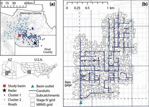
While floods and flash floods occur in both summer and winter in this urban area, pluvial flooding events caused by monsoonal thunderstorms occur more frequently than other types of flood events (Yang et al. 2017; their fig. 4) and are particularly impactful in small urban catchments with short response times. To investigate the predictability of these events, we simulate urban flooding with different radar rainfall products in an urban catchment of 2.38 km² in downtown Phoenix (Fig. 1(b)). The basin is largely (~80%) impervious and includes the dense downtown business district, the Phoenix City Hall, and entertainment venues such as the Citi Field Baseball stadium. As detailed in Fig. 1(b), the drainage infrastructure in the catchment includes 657 catch basins, 386 manholes and other junctions, and 1091 pipe segments totalling 24 km, all draining to one outlet that discharges to the Salt River south of downtown Phoenix. In addition to this surface discharge, there are 26 drywells that capture and infiltrate stormwater.

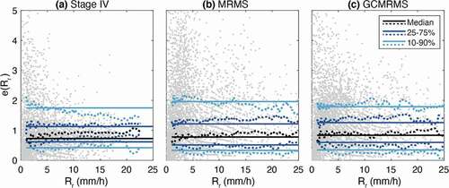
Figure 4. Relations between e(R_r) and R_r for the different radar products, along with quantiles of the empirical (dotted lines) and mixed gamma (solid lines) distributions for cluster 2

MRMS: Multi-Radar Multi-Sensor; GCMRMS: gauge corrected MRMS.

3 Datasets

3.1 Rainfall products

We use three radar-derived QPEs: Stage IV, MRMS, and GCMRMS. Stage IV QPEs are produced by processing and mosaicking reflectivity data from the NEXRAD network; rainfall rates are further adjusted with gauge and satellite observations and manually quality controlled (Y. Lin 2020). MRMS products are derived by integrating radar observations from the NEXRAD and Canadian networks, with atmospheric environmental data, satellite data, and lightning and raingauge observations (J. Zhang et al. 2016). We acquired Stage IV and MRMS QPEs for summers (July to October) of 2015–2019. For MRMS, we obtained version 11 of the radar-only and gauge-corrected (GCMRMS) products. Stage IV (MRMS; GCMRMS) QPEs are available in polar stereographic coordinates at 4-km, 1-h (1-km, 2-min; 1-km, 1-h) resolution. We project all radar products into Universal Transverse Mercator (UTM) Zone 12 N and aggregate MRMS at one-hour time resolution. To quantify errors in the QPEs and apply the multiplicative error model, we use rainfall records of 168 gauges of the Automated Local Evaluation in Real Time (ALERT) network managed by the Flood Control District of the Maricopa County (FCDMC; Fig. 1(a)). For these tipping-bucket gauges, we convert the tipping instants into rainfall intensities at one-hour resolution following the procedure described by Mascaro et al. (2013).

3.2 Geospatial datasets for hydrologic–hydraulic simulations

We set up the EPA SWMM hydrologic–hydraulic model in the study basin using several geospatial datasets. We use the terrain description from a LiDAR product at an equivalent resolution of 0.25 m that is publicly available (ASU 2018); soils data from the Natural Resources Conservation Service (NRCS) Web Soil Survey (NRCS 2019); and percent imperviousness from a 30-m map from the National Land Cover Database (MRLC 2016). We obtained information on drainage infrastructure components from the City of Phoenix, including location of pipes, dry wells, and manholes; pipe material, diameter, and slope; and elevations of pipe rim and invert.

4 Methods

In the following sections, we first describe the statistical error model used to characterize the uncertainty of radar errors, and then we illustrate the setup of the hydrologic–hydraulic model. Lastly, we detail the approach used to sample the radar rainfall error model to force the hydrologic–hydraulic model and describe the metrics adopted to quantify the associated uncertainty.

4.1 Radar rainfall error model

We use a multiplicative model to characterize the radar rainfall model uncertainty. This type of model has been shown to outperform additive models in terms of predictive skill and ability to separate systematic and random errors and capture the nonlinear relationship between the magnitude of errors and measurement (Tian et al. 2013, Tang et al. 2015). Specifically, we use the model proposed by Ciach et al. (2007) and recently improved by Villarini et al. (2014), who suggested the use of a mixture of gamma distributions instead of the Gaussian distribution to characterize positive multiplicative errors, along with techniques to account for the spatiotemporal structure of the errors. Since the errors of radar-derived products are affected by the distance from the radar, we divide the raingauges into two clusters, as shown in Fig. 1(a), and apply the model separately on each cluster. In the following, we provide a brief description of the model and refer the reader to Ciach et al. (2007) and Villarini et al. (2014) for a detailed description. We also point out that a recent study by Ciach and Gebremichael (2020) has proposed an alternative parameterization of the error model based on a three-parameter modified Laplace model.

The model assumes that the difference between area-averaged radar rainfall estimates and point gauge measurements is negligible. In a previous model application in Oklahoma by Ciach et al. (2007), this assumption was supported, referring to Ciach and Krajewski (2006), who calculated the spatial correlogram of one-hour rainfall time series observed at pairs of gauges with distances, d, of less than 4 km. These authors found the Pearson’s correlation coefficient, ρ, to be larger than 0.88, thus suggesting the rainfall spatial variability to be small within a radar pixel. We perform a similar analysis with our dataset by computing the Kendall’s τ correlation coefficient to better measure the correspondence between samples that are not well described by the Gaussian distribution (Serinaldi 2008, Villarini et al. 2014). We then derive ρ from τ using the equation $\rho =sin\left(\frac{\pi \tau }{2}\right)$ (Fang et al. 2002) and fit the power-law relation

(1) $\rho \left(d\right)={\rho }_0\mathrm{e}\mathrm{x}\mathrm{p}\left(-\frac{d}{d_0}\right)$(1)

with parameters ρ₀ and d₀, to capture the average behavior. We find ρ to be larger than 0.88 for d ≤ 1 km (the MRMS grid resolution), which is similar to the value of Ciach and Krajewski (2006) (see Fig. S1 in the Supplementary material). The minimum ρ decreases instead to 0.72 for d = 4 km, suggesting that a single raingauge may not fully capture the rainfall variability within a Stage IV pixel. Dai et al. (2018) showed that this can introduce uncertainty in the application of a different error model. Since a similar study has not been yet conducted for the model adopted here and is beyond the scope of this paper, we will continue to assume that raingauges provide a relatively accurate estimate of the area rainfall.

According to the multiplicative structure of the error model, the true rainfall value in a radar pixel, R_true, can be expressed as the product of a deterministic component, $h\left(R_r\right)$, and a random component, $e\left(R_r\right)$

(2) $R_{true}=h(R_r)\cdot e(R_r).$(2)

Both functions in Equation (2)(2) $R_{true}=h(R_r)\cdot e(R_r).$(2) depend on $R_r$, which is the radar rainfall value corrected for unconditional bias (if present), computed as:

(3) $\begin{array}{c}{R}_r=B_0\cdot {R_r}^{\ast }\end{array}.$(3)

B₀ is in turn calculated as:

(4) $\begin{array}{c}{B}_0=\frac{{\sum }_i{R}_{g,i}}{{\sum }_i{R}_{r,i}^{\ast }}\end{array},$(4)

where R_g,i is the raingauge measurement at the ith gauge, and $R_{r,i}^{\ast }$ is the biased radar rainfall in the co-located pixel (i.e. the original Stage IV, MRMS and GCMRMS values).

In Equation (2)(2) $R_{true}=h(R_r)\cdot e(R_r).$(2) , the function $h\left(R_r\right)$ provides an estimate of the bias conditioned on $R_r$, while $e\left(R_r\right)$ accounts for residual errors after removing unconditional and conditional biases. We obtain the two components as follows. We use raingauge observations, R_g, to approximate R_true; next, following Ciach et al. (2007), we compute $h\left(R_r\right)$ by (i) applying the Epanechnikov kernel with a minimum of 20 data points, and (ii) fitting the power relation:

(5) $\begin{array}{c}h\left(R_r\right)=a{R}_r^b\end{array}$(5)

with parameters a and b, to the line derived from the kernel. Equation (5)(5) $\begin{array}{c}h\left(R_r\right)=a{R}_r^b\end{array}$(5) allows obtaining the sample of errors as the ratio of R_g (approximating R_true) and $h\left(R_r\right)$. We use this sample to find the best parametric distribution to statistically model the random component $e\left(R_r\right)$, testing different mixtures of gamma distributions, as proposed by Villarini et al. (2014). For each distribution, we evaluate the possibility of using parameters that are constant or dependent on R_r and choose the most appropriate one with the Akaike information criterion (AIC; Akaike 1974).

We also test whether the random errors in our dataset exhibit significant spatial and temporal dependencies. For each cluster, we compute the spatial correlogram of the random errors using the Kendall’s τ correlation coefficient and the same power model of Equation (1)(1) $\rho \left(d\right)={\rho }_0\mathrm{e}\mathrm{x}\mathrm{p}\left(-\frac{d}{d_0}\right)$(1) , where ρ(d) and ρ₀ are now replaced by τ(d) and τ₀, respectively (Fig. S2 in the Supplementary material). We find the nugget parameter τ₀ to range from 0.23 to 0.37 depending on the radar product, thus indicating that the correspondence between errors at close pixels is rather low. To verify this assumption, we (i) generate 100 spatially correlated error fields, following Villarini et al. (2014), as well as 100 random error fields; and (ii) compute for each field the basin mean areal rainfall during four selected storms (see Section 4.3). We find the uncertainties of the basin mean areal rainfall derived from spatially correlated and uncorrelated fields to be very similar (not shown). To quantify the temporal dependencies, we compute the autocorrelation of the errors for N = 462 storms (detected in 85 individual pixels) with durations longer than four hours. We then compare the resulting median and 90% confidence interval with those of N time series of random white noise with the same duration as the observed events. We find that – apart from MRMS, which exhibits a certain degree of autocorrelation at lag 1 – observed and synthetic autocorrelations are similar (Fig. S3 in the Supplementary material). Based on these empirical outcomes, we consider the spatiotemporal dependencies among the random errors to be negligible for the purpose of applying the error model in our basin.

4.2 The coupled hydrologic–hydraulic model

4.2.1 Brief model description

SWMM is a semi-distributed rainfall–runoff model developed by the US EPA (Koustas 2000) for simulating runoff in urban catchments. The model includes a hydrologic component that transforms rainfall into surface runoff in sub-catchments, and a routing component that transports this runoff through stormwater infrastructure elements, including pipes, channels, and storages. As detailed in the user’s guide (W. James et al. 2010), different hydrologic processes can be simulated that allow applying the model in event-based or continuous fashion. The routing component includes several hydraulic modeling capabilities largely based on the application in 1D of the momentum and continuity equations. The model domain is generated by (i) discretizing the catchment into smaller sub-catchments corresponding to each inlet into the infrastructure drainage system; and (ii) introducing different types of model elements, such as conduits, junctions (e.g. catch basins and manholes), outfall nodes, and storage units (see Table 1 for a description of the main elements). Model inputs include rainfall data, provided through one or more raingauges (or radar pixels; see Table 1), while outputs include the flow rate and hydraulic grade lines throughout the drainage system, and surface flood volumes when surcharge occurs (i.e. water rises above the crown of the highest conduit) and the hydraulic grade line exceeds surface elevation of the junctions.

Table 1. Description of the main components of the Storm Water Management Model (SWMM) hydrologic–hydraulic model

Component	Description
Raingauges	Point measurements of rainfall over the duration of the modeling period from an actual raingauge or a radar pixel. Each sub-catchment is assigned rainfall from the closest gauge or radar pixel center.
Sub-catchments	Hydrologic units of land delineated based on the local topography.
Conduits	Pipes or channels through which water is transported. This includes culverts and underground storm pipes.
Junctions	Drainage nodes that connect conduits to each other. Culvert inlets and outlets, pipe inlets and outlets, and manholes are all modeled as junctions. Junction properties include rim (surface) and invert (conduit base) elevations.
Outfall nodes	Drainage nodes at the downstream boundary of the catchment.
Storage units	Drainage nodes with an associated storage volume available.

In addition to the standard components of SWMM, we also use the proprietary PCSWMM implementation to model overland routing of flood water and the resulting flood extent. This is accomplished through an integrated 1D–2D modeling approach where the fully dynamic 1D approach (i.e. SWMM) is extended to 2D free surface flow using a mesh that captures topography, geometry, and built structures. PCSWMM builds upon the SWMM 1D model and discretizes the domain into a square mesh where each 2D cell is represented with a 2D node or a junction, whose invert elevations are assigned as either the ground surface elevation or the rim elevation of adjacent coupled 1D junctions (Finney et al. 2012, R. James et al. 2013). In PCSWMM, rainfall–runoff processes and routing in the pipe system are simulated in 1D, as in SWMM. When flood conditions are simulated, water leaves the drainage system at catch basin junctions (and manholes, if not bolted) and is then routed on the 2D mesh cells. Flood water is routed across the land surface and, as the hydraulic grade line drops below the catch basin rim elevation, water can re-enter the drainage system.

4.2.2 Model setup

To set up SWMM in our basin, we extensively pre-process and quality control the LiDAR and infrastructure data through geographic information system (GIS) software and field visits. We use the LiDAR point cloud data with an average point spacing of 0.25 m and a total point count of over 37.8 million in the basin to generate a digital elevation model (DEM) at 0.6-m resolution for the catchment delineation. The elevations of the point cloud data range from 320 to 484 m, mainly constituting returns from the road surface and roofs of the buildings. Features such as buildings are initially retained as they can influence sub-catchment boundaries. Next, we use the high-resolution DEM to generate 2D computational square grid cells at a lower resolution of 4.57 m (15 ft) for overland routing of flood waters needed for PCSWMM. This lower resolution is selected due to the high computational demands of routing overland flow. We then exclude buildings through a mask of building footprints available from ASU (2018), as they would artificially raise the grid cell elevation and impact overland flow routing. Using aerial imagery, we visually identify DEM and 2D cells with abnormally low or high elevations caused by the presence of overpasses or sites that were under construction when the LiDAR was obtained. To prevent ponding at these artificial depressions, those sections are excluded from the 2D computational grid by creating bounding layers over them.

As a next step, we check the reliability of the GIS data of stormwater infrastructure components through field visits. During these, we verify surface structures (e.g. catch basins, manholes) in frequently flooded areas identified by project partners in the City of Phoenix and the FCDMC, as well as areas that deviated from standard design practice. In addition, we identify a few missing or moved surface components, including catch basins and manholes, as well as missing subsurface components where stormwater could not reach the outlet from a portion of the system as documented. These missing pipe segments are specified based on design standards. Additionally, some components have missing attribute data such as rim or invert elevations, slope, pipe diameter, and pipe material. Rim elevations are estimated from the DEM, while invert elevations, slope, pipe size, and material are estimated from adjacent components and design standards. Once data gaps are assessed and filled, the infrastructure shapefiles are imported into SWMM to create the drainage network in the model. Finally, pipe material (mostly concrete) is used to specify Manning’s roughness coefficient (on average, 0.011).

We apply the model for event-based simulations using rainfall data from (i) the only gauge of the FCDMC networks installed within the basin; and (ii) the radar grids (see Fig. 1(b)). For the hydrologic component, we specify the percent imperviousness of each sub-catchment using the NRCS dataset and we simulate infiltration with the Green-Ampt method, which is parameterized with soil properties from the Web Soil Survey database. Parameter values are reported in Tables 2 and 3. The sub-catchments draining to each of the 26 drywells present in the basin are modeled as disconnected from the rest of the drainage system unless flooding and overland flow cross sub-catchment boundaries (modeled only in the 2D PCSWMM). We use the 1D dynamic wave routing method to model routing in the pipes. PCSWMM simulates surface flooding by coupling the 1D model of the drainage network with a 2D overland flow model. When surcharge occurs, flow exiting catch basins (all manholes are bolted in our study basin) is routed on the 4.57 m × 4.57 m mesh surface using the St Venant flow equations.

Table 2. Parameter values of the Green-Ampt infiltration scheme adopted in Storm Water Management Model (SWMM)

Soil types	Percentage of basin area	Suction head (cm)	Conductivity (cm/h)	Initial deficit
Avondale clay loam	1.2	38.53	0.15	0.21
Estrella loam	0.3	38.02	0.43	0.14
Gilman loam, 1–3% slope	15.2	43.03	0.30	0.15
Glenbar clay loam	40.2	53.87	0.15	0.19
Laveen loam, 0–1% slope	34.4	36.50	0.61	0.11
Mohall clay loam	8.7	42.24	0.18	0.19

Table 3. Imperviousness and ground slope values assigned to the sub-catchments, summarized as a range of values for percentages of the basin area

Imperviousness (%)	Percentage of basin area
0–50	7.8
51–60	10.0
61–70	19.6
71–80	35.1
81–100	27.5
Ground slope (%)	Percentage of basin area
0–5	16.5
6–10	75.2
11–65	8.3

4.3 Hydrologic–hydraulic simulations

We identify four storm events from the 2015–2019 study period with significant areal coverage in Phoenix and relatively high average precipitation depth, and for which NOAA has reported impacts on traffic and properties (NOAA 2021). The storm characteristics are presented in Table 4. Two storms occurred in the middle of the NAM season and, as such, are of monsoonal origin; the other two were observed at the end of September and in October during the transition from NAM to winter weather conditions and, for one of them, the source of moisture came partially from a tropical storm (personal communication with Dr. Larry Hopper, at the NWS). Storm durations range from 6 to 30 hours and gauge total rainfall varies from 5 to 10 mm. The impacts of one of the storms (23 September 2019) on street-level flooding in the study basin are presented in the photograph (Fig. 2) that was taken with a camera installed to monitor flooding during the event. For each storm, we conduct simulations with SWMM using different rainfall inputs at one-hour resolution, including (i) raingauge observations (R_g); (ii) original (i.e. R_r*) QPEs from Stage IV, MRMS and GCMRMS; and (iii) an ensemble of N = 100 fields generated through the error model for each radar product. The rainfall inputs derived from the raingauge are spatially uniform, while those produced by the original radar products and the error model are spatially variable with a resolution of 4 km (1 km) for Stage IV (MRMS and GCMRMS), as also shown in Fig. 1(b). The procedure used to generate N = 100 fields with the error model is based on Monte Carlo simulations, consisting of the following steps:

1. For a given storm with T time steps, the unconditional bias is first removed from the original radar estimates using Equation (3)(3) $\begin{array}{c}{R}_r=B_0\cdot {R_r}^{\ast }\end{array}.$(3) , and the deterministic component $h\left(R_r\right)$ is calculated with Equation (5)(5) $\begin{array}{c}h\left(R_r\right)=a{R}_r^b\end{array}$(5) at all pixels and times.

2. Since the spatiotemporal dependencies of the errors are found to be negligible, for each pixel, a total of T random errors, $e\left(R_r\right)$, are randomly generated from the corresponding probability distribution.

3. The errors and the deterministic component $h\left(R_r\right)$ are then used to estimate the true rainfall using Equation (2)(2) $R_{true}=h(R_r)\cdot e(R_r).$(2) , resulting in T rainfall grids for each pixel. This spatiotemporal rainfall field represents a possible realization of the true rainfall for the analyzed event, given the original radar-derived QPEs. The spatiotemporal rainfall field is then used to force SWMM.

4. Steps 2 and 3 are repeated N times.

Table 4. Summary of storm characteristics, including start and end date and time in Coordinated Universal Time (UTC), identified as the times when (i) any of the gauge and radar products started measuring nonzero rainfall in the basin and (ii) all measured zero rainfall, respectively; type as defined by Dr. Larry Hopper from National Weather Service (NWS) (2020; personal communication); duration; rainfall totals observed by gauges (R_g); and original (R_r*) and bias corrected (in parentheses; R_r) mean areal rainfall totals of the radar-derived estimates

Start date	End date	Type	Duration (h)	Gauge (mm)	Stage IV (mm)	MRMS (mm)	GCMRMS (mm)
24 July 2017 02:00	24 July 2017 20:00	Monsoon	18	7.0	7.0 (8.9)	13.1 (8.6)	15.7 (11.4)
31 July 2018 03:00	31 July 2018 09:00	Monsoon	6	5.0	5.8 (7.4)	20.0 (13.1)	11.0 (8.3)
7 October 2018 08:00	7 October 2018 19:00	Transition	11	10.0	10.0 (12.6)	17.1 (11.2)	7.1 (5.3)
23 September 2019 10:00	24 September 2019 19:00	Tropical/ transition	33	6.0	6.8 (8.7)	15.8 (10.4)	8.6 (6.5)

Figure 2. Flooding in the study catchment at Central Ave and Washington St in Phoenix, AZ during the storm on 23 September 2019

Since the 2D simulations with PCSWMM are computationally intensive, running this model N = 100 times is not feasible. Therefore, we select three rainfall sequences generated from the previous Monte Carlo SWMM simulations for each storm. These sequences correspond to the 25th, 50th, and 75th percentiles of the distribution of the total flood volume, V_f (i.e. the volume of water that exits the drainage system through catch basins when the hydraulic grade line exceeds the rim elevation of catch basins) across the 100 Monte Carlo runs. We then apply PCSWMM for these three realizations for each storm to illustrate the influence of precipitation uncertainty on flood extent in a computationally efficient manner.

4.4 Uncertainty quantification

Let {x₁, …, x_N} be the values of a given variable x (rainfall or discharge at a given time step) returned by the ensemble runs with the radar rainfall or the hydrologic model. We quantify the uncertainty of these ensemble simulations of x through two simple metrics: (i) the skewness of the distribution of {x₁, …, x_N}; and (ii) the interquartile range relative to the median: RIQR = (q_0.75−q_0.25)/q_0.50 × 100, where q_p is the quantile of the empirical distribution of {x₁, …, x_N} associated with the non-exceedance probability p.

5 Results

5.1 Characterization of radar QPE uncertainty

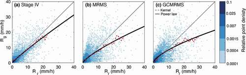
The first step to apply the error model is to calculate the unconditional bias, B₀, which is needed to compute R_r via Equation (3)(3) $\begin{array}{c}{R}_r=B_0\cdot {R_r}^{\ast }\end{array}.$(3) . We find B₀ to be 1.26, 0.66, 0.76 for Stage IV, MRMS, and GCMRMS, respectively, indicating that original Stage IV (MRMS and GCMRMS) QPEs underestimate (overestimate) the gauge observations. Figure 3 presents the scatterplots between R_r and R_g (estimating the true rainfall, R_true) along with the lines obtained through the Epanechnikov kernel and the power law of Equation (5)(5) $\begin{array}{c}h\left(R_r\right)=a{R}_r^b\end{array}$(5) for cluster 2 (results for cluster 1 are reported in Fig. S4 of the Supplementary material). All radar products exhibit a positive systematic bias that becomes larger as R_r increases, as found in previous work (e.g. Ciach et al. 2007, Villarini and Krajewski 2009, 2010b, Villarini et al. 2014). The conditional bias for Stage IV QPEs is much smaller than that found for the MRMS and GCMRMS products. The errors for GCMRMS are slightly smaller than those of MRMS for R_r ≤ 15 mm/h, where most data points lie; the opposite is true for R_r > 15 mm/h, although fewer points exist in this region.

Figure 3. Scatterplots of radar rainfall estimates, R_r, and true rainfall approximated by the gauge estimates, R_g, for cluster 2. A total of 8645, 8859, and 8605 nonzero pairs for (a) Stage IV, (b) Multi-Radar Multi-Sensor (MRMS), and (c) gauge corrected MRMS (GCMRMS) are shown using different colors based of their relative frequency. In each panel, the dashed red line is the systematic component estimated with the Epanechnikov kernel, and the solid black line is the power law of Equation (5)(5) $\begin{array}{c}h\left(R_r\right)=a{R}_r^b\end{array}$(5) . Parameters of the power law are a = 1.12, b = 0.90 for Stage IV; a = 1.37, b = 0.77 for MRMS; and a = 1.86, b = 0.66 for GCMRMS

As a next step, we use Equation (2)(2) $R_{true}=h(R_r)\cdot e(R_r).$(2) to compute the errors, e(R_r), quantifying the variability of radar rainfall estimates around the h(R_r) lines. Figure 4 shows the errors along with the empirical quantiles (dotted lines) derived with the Epanechnikov kernel for cluster 2 (results for cluster 1 are reported in Fig. S5 of the Supplementary material). For all products, the distribution of the errors is positively skewed and, importantly, does not vary with R_r. Based on this empirical outcome, we adopt a parametric distribution with constant parameters (i.e. a distribution that does not change with R_r), as in Villarini et al. (2014). We find the mixture of three gamma distributions to be the most appropriate parametric distribution, as suggested by the lowest AIC values (see Supplementary material, Table S1). The quantiles derived from the mixed gamma distribution are shown in Fig. 4 with solid lines, while the comparison between empirical and parametric distributions is reported in Fig. 5 (see Fig. S6 in the Supplementary material for cluster 1) and parameters of the gamma distribution for each radar product are summarized in Table 5. Figure 5 reveals that, for all products, the distribution of the errors is very well reproduced up to about e(R_r) = 5; larger values of e are underestimated, but they only account for less than 0.5% of the sample.

Table 5. Parameters of the mixture of three gamma distributions used to characterize the distribution of errors, $f\left(e;w_1,{\alpha }_1,{\beta }_1,w_2,{\alpha }_2,{\beta }_2,w_3,{\alpha }_3,{\beta }_3\right)=\sum _{j=1}^3{w}_j\cdot g\left(e;{\alpha }_j,{\beta }_j\right)$, where $g\left(e;{\alpha }_j,{\beta }_j\right)$ is the probability density function of the jth gamma distribution of the errors, e (for simplicity, we dropped the dependence on R_r). Parameter values are reported for clusters 1 (C1) and 2 (C2)

Parameter	Stage IV		Multi-Radar Multi-Sensor(MRMS)		gauge corrected MRMS(GCMRMS)
	C1	C2	C1	C2	C1	C2
α1	1.34	6.50	2.89	5.16	1.55	1.76
α2	55.34	1.26	13.58	1.09	11.75	19.93
α3	19.97	357.00	6.50	9.18	35.85	38.16
β1	0.95	0.14	0.29	0.14	0.72	0.60
β2	0.01	1.08	0.17	1.10	0.07	0.04
β3	0.05	0.002	0.55	0.21	0.04	0.04
w1	0.47	0.46	0.92	0.64	0.47	0.61
w2	0.37	0.33	0.05	0.23	0.43	0.31
w3	0.16	0.21	0.03	0.13	0.10	0.08

Figure 5. Comparison of survival functions of the empirical distribution and mixture of three gamma distributions for cluster 2

MRMS: Multi-Radar Multi-Sensor; GCMRMS: gauge corrected MRMS.

5.2 Propagation of uncertainty from rainfall to runoff

5.2.1 Rainfall uncertainty

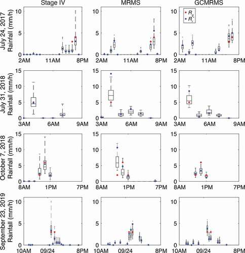
Figure 6 presents, for each storm, the time series of rainfall recorded at the gauge (R_g; red dots) along with the basin mean areal rainfall estimated by the three radar QPEs (R_r*; blue dots) and simulated by the corresponding error model (box plots displaying 50% and 90% confidence intervals of N = 100 values produced by the Monte Carlo runs). For all events, the radar products estimate nonzero rainfall in a larger number of time steps as compared to the gauge. For the gauge-corrected Stage IV, R_g is very close to both R_r* and the median of the Monte Carlo simulations. As discussed, MRMS QPEs are positively biased, so that R_r* is in most cases larger than R_g and median of the error model simulations. This bias is reduced when the gauge correction is applied in GCMRMS (see e.g. the event on 10 July 2018). For all three products, higher rainfall measurements yield a higher magnitude of uncertainty for the error model. Finally, Table 6 presents the mean skewness and RIQR of the ensemble hourly rainfall across each storm duration. Due to the positive skewness of the distribution of the residual error in the radar error model (see Fig. 4), the mean skewness of the simulated rainfall is also positive and included between 1.0 and 3.2, with higher values for Stage IV, followed by MRMS and GCMRMS. The relative variability across the ensemble members is quantified via the RIQR, whose average ranges from 56.1% to 74.6%, with the highest (lowest) values found again for Stage IV (GCMRMS).

Table 6. Quantification of uncertainty of simulated rainfall and runoff via skewness and RIQR of the ensemble rainfall and discharge at the basin outlet (in parentheses) averaged across each event duration (i.e. skewness and RIQR are computed for each time step and then averaged in time). Values are reported for each radar product

Storm start date	Stage IV	MRMS	GCMRMS		Stage IV	MRMS	GCMRMS
	Skewness (-)				RIQR (%)
	Rainfall (discharge at the outlet)
24 July 2017	3.2 (2.0)	1.7 (1.1)	1.4 (0.4)		71.0 (66.9)	68.4 (51.6)	59.5 (22.4)
31 July 2018	2.9 (0.8)	1.5 (1.0)	1.5 (0.9)		70.1 (45.0)	68.2 (43.7)	69.2 (41.1)
7 October 2018	2.1 (0.9)	1.7 (1.3)	1.0 (0.5)		59.7 (55.8)	67.9 (49.0)	41.5 (27.4)
23 September 2019	2.6 (2.5)	1.7 (0.9)	1.3 (0.5)		74.6 (47.0)	70.2 (78.0)	56.1 (50.3)

MRMS: Multi-Radar Multi-Sensor; GCMRMS: gauge corrected MRMS.

Figure 6. Time series of rainfall recorded at the gauge (R_g), basin mean areal rainfall estimated by the three radar products (R_r*), and box plots of the N = 100 Monte Carlo simulations of the radar rainfall error model for the four events in Table 2. Boxes and whiskers of the box plots show the 50% and 90% confidence intervals, respectively, while the horizontal line is the median. Times are in UTC.

MRMS: Multi-Radar Multi-Sensor; GCMRMS: gauge corrected MRMS

5.2.2 Uncertainty of basin-integrated runoff

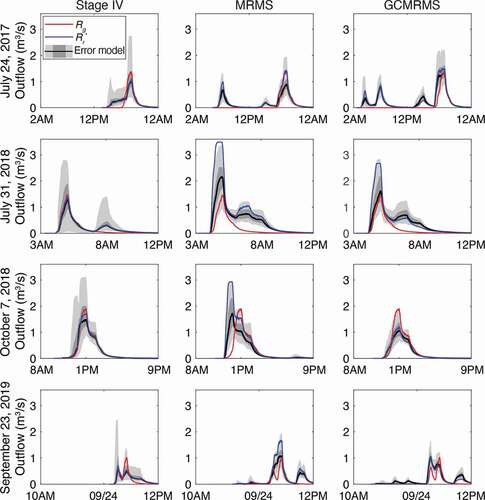
We start evaluating the propagation of rainfall uncertainty into runoff by first assessing the variations in the outlet hydrograph (i.e. outflow at the pipe that discharges to the Salt River) across radar products and storms. The hydrographs simulated by the SWMM model under the rainfall forcings of Fig. 6 are displayed in Fig. 7. The use of Stage IV QPEs and raingauge observations as inputs for SWMM leads to closely aligned hydrographs, which are also very similar to the median hydrograph of the corresponding ensemble simulations. In contrast, the outflow generated by the original MRMS QPEs is consistently biased high compared to the simulation under the gauge rainfall observations, with the median of ensemble runs falling between the two. As found in Fig. 6 for the rainfall values, the gauge correction of MRMS QPEs reduces the bias in the resulting flow, as shown in the hydrographs with GCMRMS forcings. The uncertainty of the ensemble hydrologic simulations is quantified in Table 6 via the time-averaged skewness and RIQR of the discharge at the outlet. The mean skewness is still positive, with values in the range 0.4–2.5, which are lower compared to those found for rainfall. This is also true for the mean RIQR that varies from 22.4% to 66.9%. Metric values are, again, the largest (smallest) for Stage IV (GCMRMS).

Figure 7. Hydrographs simulated by the SWMM model at the pipe located at the catchment outlet under rainfall recorded at the gauge (R_g), original radar QPEs (R_r*), and an ensemble of rainfall fields generated with the error model. The corresponding N = 100 outflow simulations are plotted with shaded areas showing the 50% (light gray) and 90% (dark gray) confidence intervals, while the black line is the median.

MRMS: Multi-Radar Multi-Sensor; GCMRMS: gauge corrected MRMS

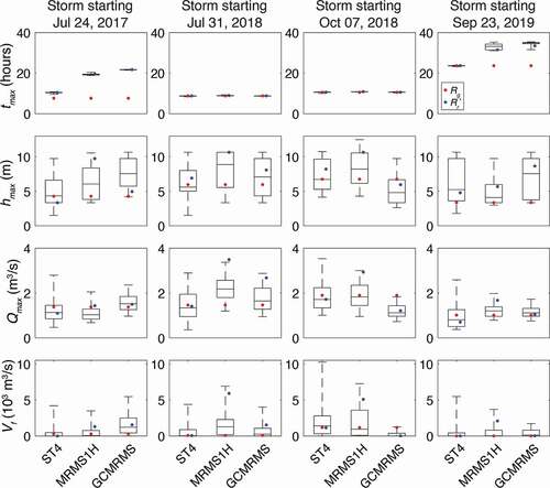
To complement the information provided by the hydrographs at the catchment outlet and better assess flood impacts and differences across precipitation inputs, we examine additional metrics simulated by SWMM. These include Q_max: peak flow of the hydrograph at the outlet; and V_f: stormwater volume that ponds on the surface of the catchment when the hydraulic grade line reaches the catch basin rim elevation at one or more locations. In addition, we consider two metrics that characterize the hydraulic response of the stormwater pipe system under surcharge conditions; these are t_max: maximum total duration of node surcharging across all nodes; and h_max: maximum height of the hydraulic grade line above the pipe invert level. Note that nonzero values for t_max and h_max do not necessarily imply surface flooding, as mentioned in Section 4.2.1. Figure 8 presents the simulated metric values for each storm and radar product. Simulations under gauge rainfall, R_g, could be used as reference to compare across storms. The lowest (highest) Q_max and V_f are obtained for the storm on 23 September 2019 (7 October 2018), which are characterized by the lowest (highest) rainfall intensity (see Table 4). h_max exhibits a certain relation with Q_max and V_f, which quantify actual surface flooding, while t_max is largely controlled by storm duration (reported in Table 4). Turning our attention now to the radar products, all metrics modeled with R_g are close to those simulated under Stage IV R_r* and in most cases (all cases except t_max for event 1) within the 50% (90%) confidence interval of the ensemble runs. When compared to the metrics simulated under R_g, simulations with MRMS rainfall products lead to longer t_max in two events and larger h_max,Q_max,V_f in most storms. The use of GCMRMS improves MRMS performance, apart from some metrics in individual storms (e.g. h_max on 23 September 2019; V_f on 24 July 2017). Finally, when considering the spread of the ensemble distributions, there is not a specific radar product that leads to wider or narrower distributions for a given metric across all events. These metrics are further discussed in Section 6.

Figure 8. Flood metrics simulated by one-dimensional SWMM for the selected storms with rainfall recorded at the gauge (R_g), original radar QPEs (R_r*), and ensemble of rainfall fields generated with the error model plotted through box plots (boxes and whiskers show the 50% and 90% confidence intervals, respectively). See the text for definitions of the flood metrics. t_max is measured in hours since the simulations started

MRMS: Multi-Radar Multi-Sensor; GCMRMS: gauge corrected MRMS; SWMM: storm water management model.

5.2.3 Uncertainty of spatial flooding

The metrics presented in Fig. 8 aid in comparing model output across simulations. However, information on location and extent of flooding over time is needed to alert residents to dangerous conditions, provide timely emergency response, and identify critical locations for infrastructure investment. Such information is obtained through the 2D simulations of flood routing with PCSWMM. Figures 9 and 10 illustrate the uncertainty in maximum flood extent (i.e. areas that are flooded for at least one time step) simulated under each radar product for the storms on 31 July 2018 and 7 October 2018, respectively (Figs S7 and S8 in the Supplementary material show results for the other two storms). Uncertainty is captured through the simulations under the rainfall fields of the error model associated with the 25th percentile (blue), median (green), and 75th percentile (red) of the distribution of V_f from the 1D SWMM simulations. Thus, if a pixel is blue, flooding has been simulated for all higher percentiles; when it is green, it has been simulated for the median and 75th percentile; and when the pixel color is red, flooding only occurred for the 75th percentile.

Figure 9. Uncertainty of flood extent maps for the storm on 31 July 2018, simulated by PCSWMM under (a–c) Stage IV, (d–f) MRMS, and (g–i) GCMRMS products

MRMS: Multi-Radar Multi-Sensor; GCMRMS: gauge corrected MRMS.

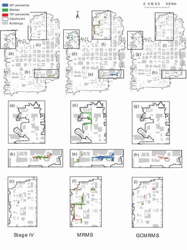
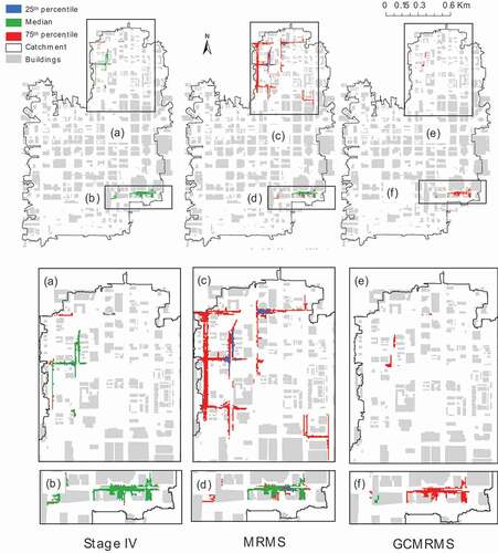
For the monsoonal storm on 31 July 2018, the use of rainfall fields generated by the error model with Stage IV QPEs (Fig. 9(a–c)) leads to simulation of street flooding in two distinct basin locations (Fig. 9(b,c)), with a total of 0.001, 0.03, and 0.05 km² of flooded areas for the 25th percentile, median and 75th percentile, respectively. If rainfall forcings are provided by MRMS (Fig. 9(d–f)), street flooding is also predicted in a location in the upper part of the basin (Fig. 9(d,f)). Given the positive bias of these QPEs, the simulated flooding extent is larger and equal to 0.07 (0.23) km² for the 25th (75th) percentile. Interestingly, the uncertainty across the percentiles is low in a relatively large region in the lower part of the catchment (blue area in Fig. 9(e)). The gauge correction of MRMS QPEs performed for GCMRMS leads to results that are substantially similar to those for Stage IV (Fig. 9(g–i)). Maps of flooded areas for the transition storm on 7 October 2018 are reported in Fig. 10. Flooding is predicted in two of the same basin regions displayed in Fig. 9. Flooded areas under Stage IV (Fig. 10(a,b)) are very similar for the median (0.16 km²) and 75th percentile (0.19 km²), while they decrease substantially for the 25th percentile (0.006 km²). As found for the monsoonal storm of Fig. 9, using MRMS QPEs (Fig. 10(c,d)) as model inputs increases the extent of street-level flooding as compared to Stage IV, which reaches 0.04 (0.4 km²) for the 25th (75th) percentiles. The adoption of GCMRMS (Fig. 10(e,f)) leads instead to lower flooded areas compared to Stage IV, ranging from no flooded areas for the 25th percentiles to 0.09 km² for the 75th percentile.

Figure 10. Uncertainty of flood extent maps for the storm on 7 October 2018, simulated by PCSWMM under (a–c) Stage IV, (d–f) MRMS, and (g–i) GCMRMS products

MRMS: Multi-Radar Multi-Sensor; GCMRMS: gauge corrected MRMS.

6 Discussion

While focused on an urban catchment in the Phoenix metropolitan area, the results of our modeling efforts are based on extensive precipitation, land surface, and infrastructure datasets, and, as such, they provide general insights on the utility of radar QPEs and hydrologic–hydraulic models for urban flood predictions in the NAM region and other areas, as discussed in the next subsections.

6.1 Comparison of radar products and their utility for urban flood modeling

When applying the error model using the network of 168 gauges, we find that, on average, Stage IV QPEs underestimate gauge rainfall by ~20%, while MRMRS and GCMRMS overestimate it by about 51% and 31%, respectively (see values of B₀ reported in Section 5.1). Qualitatively, this result is confirmed for the four simulated storm events. Our finding is consistent with the extensive comparison of six radar products, including Stage IV and earlier versions of MRMS and GCMRMS, performed by Seo et al. (2018) in Iowa, but opposite to two separate analyses, by Lin et al. (2018) and Gao et al. (2021), in Texas during a set of flood events. The existence of regional differences in performance of Stage IV and MRMRS have been recently highlighted in another comparison study in Louisiana by Sharif et al. (2020). Overall, our results and those of other studies suggest that radar-only QPEs are critically improved through gauge-based bias corrections, as done in Stage IV and GCMRMS.

Figure 6 shows that nonzero rainfall is observed by the radar QPEs in more time steps compared to the single point measurement of the gauge, indicating that, even in a very small basin, a single gauge may be unable to monitor localized monsoonal convective storms. Despite this, Figs 6 and 7 show that flood simulations under the more accurate Stage IV-derived rainfall products lead to very similar outcomes to those obtained with gauge rainfall, R_g. This suggests two considerations. First, while the basin area is small, the presence of stormwater infrastructure acts as an integrator of the rainfall spatiotemporal variability, so that, despite differences between R_g and Stage IV QPEs, the resulting flood simulations are substantially quite similar. Second, an important consequence of the first consideration is that, when gauge observations are not available, hydrologic simulations with Stage IV QPEs (available throughout the country) can provide a reliable reference for evaluating the impacts of urban flooding. On the other hand, in our study basin, the use of MRMS QPEs consistently results in the largest flood volumes and extents, while the flooding impacts simulated with GCMRMS QPEs are similar to those obtained with Stage IV (see Figs 8–10). Thus, our work demonstrates that the gauge correction applied to MRMS greatly improves the utility of this radar-only product for flood modeling.

6.2 Uncertainty of radar rainfall and corresponding urban flood simulations

Radar QPEs can provide key support for urban flood forecasting and management, complementing gauge observations that may only be available at sparse locations and not in real time. However, radar products are affected by different sources of errors, thus requiring models to characterize the associated uncertainty. Here, we use an error model with a multiplicative structure that leads to the largest uncertainties for the highest rainfall values (see Fig. 6), as also found in previous applications (Villarini et al. 2014). As a consequence, the uncertainty of urban flood predictions is expected to also be relatively high, as these higher precipitation observations are more likely to result in flooding. This is in general confirmed by our results, because the largest spread of the basin outflow confidence intervals occurs right after the highest rainfall events (see Figs 6 and 7). However, a closer look at the uncertainty metrics for rainfall and discharge reported in Table 6 suggests that the hydrologic processes governing the rainfall–runoff transformation have two effects: (i) they smooth the impact of the highest rainfall values simulated by the error model, so that the distribution of the ensemble outflows is more symmetric (i.e. less positively skewed) than the distribution of the rainfall inputs, as also found by Grimley et al. (2020); and (ii) they reduce the relative spread of the ensemble rainfall distribution, as shown by the mean RIQR decreasing from an average of 64.7% to 48.2% when considering all events and radar products. These conclusions should be refined in future work quantifying the effect of other sources of uncertainty for the hydrologic–hydraulic model.

We also highlight that the uncertainty of the basin outflow is greater in the rising than the falling limb of the hydrographs (Fig. 7). Specifically, across all storms and radar products, the 50% (90%) confidence interval range in the falling limb is, on average, just 8.8% (6.3%) of the range in the rising limb. This behavior can be explained considering that, in highly impervious areas and small watersheds, the rising limb and its associated uncertainty are strongly shaped by the rainfall rate. In contrast, during the falling limb of the hydrograph, catchment and drainage network properties exert a larger control that results in an uncertainty reduction. When considering the other flood metrics characterizing surface flooding and surcharge conditions in the stormwater infrastructure, we find that their uncertainty varies substantially (Fig. 8). As expected, the variability of Q_max is related to the QPE uncertainty, although the ensemble distributions for Q_max are more symmetric for the same reasons mentioned above. The distribution of V_f is highly skewed with several zero values, despite the fact that t_max and h_max are never zero. This implies that a fraction of QPEs with lower values lead to surcharge conditions but not to surface flooding. The uncertainty of t_max is practically negligible, indicating that all precipitation inputs lead to surcharge conditions over very similar maximum durations. In contrast, h_max, which quantifies the severity of surcharge conditions, exhibits a variability (mainly in the range of 5 m) due to the different QPE values simulated by the error model.

6.3 Utility for urban flood management

Urban pluvial flooding is characterized by localized damage to property and impacts to pedestrian and vehicle travel. Timely information on the location and severity of these hazards can enable response and limit travel delays and risks (NWS 2021). Our simulations with PCSWMM show that, despite uncertainties and biases across radar products, all of them robustly identify the same basin regions experiencing flooding conditions (Figs 9, 10, S7 and S8). This is a promising result supporting the operational use of QPFs derived from radar QPEs combined with hydrologic–hydraulic models, as also highlighted by Grimley et al. (2020) when discussing their simulation of pluvial flooding in an urban area in Iowa. However, the extent of flooding areas exhibits differences both for the same radar product and across radar products. The latter differences can be significant when the QPE bias is high, as found for MRMS. Therefore, flood response can confidently target the correct areas within a few blocks, though the precise flood extent remains uncertain. Improvements in QPEs accuracy are then expected to greatly benefit prioritization and response measures during floods. These findings are driven by both catchment topography and the design of the drainage network; therefore, the flood management implications of the residual uncertainty may vary by location.

It must also be noted that the SWMM model has its own structural and parametric uncertainties (Deletic et al. 2012, Abily et al. 2016). While fully assessing these is beyond the scope of the current analysis, it is important to consider that the uncertainty in flood estimates simulated in our study for an ensemble of QPEs incorporates other uncertainty sources in the SWMM model. The flood metrics and maps (Figs 8–10) also point to the need for flood extent and depth data in urban areas to properly validate the accuracy of these hydrologic and hydraulic simulations. New hydrological sensing approaches such as citizen science (Assumpção et al. 2018, Fava et al. 2019) and image-based sensing (Tauro et al. 2017, Hostache et al. 2018) offer opportunities to sense flooding as it occurs at the urban scale. These emerging approaches could enable error assessment of the urban hydrological model, providing further context to interpret the propagation of precipitation uncertainty into urban flooding.

7 Conclusions

The small size and heterogeneity of urban catchments, combined with the short, high-intensity precipitation events that drive pluvial flooding, make accurate and efficient urban pluvial flood modeling an ongoing research challenge (Blanc et al. 2012, van Dijk et al. 2014, Bermúdez et al. 2018). This is especially true in the NAM region, which is dominated by high-intensity convective thunderstorms. In this work, we provide insights on pluvial flooding by assessing the propagation of radar precipitation uncertainty into flood modeling in a 2.38-km² urban catchment in Phoenix, Arizona. Our results, based on simulations for four events during the NAM, can be summarized as follows:

1. While Stage IV QPEs slightly underestimate gauge rainfall (on average, by 20%), the resulting flood predictions are similar to those obtained with raingauge records, suggesting that Stage IV QPEs are reliable products for modeling urban flooding. MRMS QPEs are positively biased (+51%), and so are the flood peaks and extent of flooded areas simulated with these products. The gauge correction performed in GCMRMS leads to results similar to Stage IV.

2. The QPE uncertainty simulated by the error model increases with rainfall rate and is rather alike across the three radar products. This is also true for the resulting flood metrics.

3. As a result of the rainfall–runoff transformation processes and the presence of stormwater infrastructure, uncertainty of flood metrics is reduced and less positively skewed when compared with the QPE uncertainty. The uncertainty may vary significantly depending on the metrics that capture different flooding features (e.g. pipe flow, surface flooding, and pipe surcharge conditions).

4. All radar products lead to the identification of the same flooded areas within the extent of a few blocks in the basin. This is a promising result for the use of radar-derived QPEs and hydrologic–hydraulic models for urban pluvial flood modeling. However, the exact location and extent of flooded areas may vary significantly across products, suggesting that increasing QPE accuracy can greatly benefit flood management and forecasting agencies.

Acknowledgements

We thank two anonymous reviewers whose comments helped improve the quality of the manuscript. We also thank Dr. Larry Hopper and Mr. Paul Iñiguez from the NWS Phoenix Office for their insights on quality of radar QPEs and selection of storm events in the Phoenix metropolitan regions.

Disclosure statement

No potential conflict of interest was reported by the author(s).

Supplementary material

Supplemental data for this article can be accessed here.

Additional information

Funding

This work was supported by the National Science Foundation (NSF) Award “SCC: Community-Based Automated Information for Urban Flooding” (Award 1831475), and by the UCAR COMET Award “Assessing the Accuracy of Multi-Radar/Multi-Sensor (MRMS) Precipitation Estimates in the Phoenix Metropolitan Area to Support Flash Flood Warning Operations” (Award SUBAWD001574).

References

- Abily, M., et al., 2016. Spatial Global Sensitivity Analysis of High Resolution classified topographic data use in 2D urban flood modelling. Environmental Modelling & Software, 77, 183–195. doi:https://doi.org/10.1016/j.envsoft.2015.12.002.
- Adams, D.K. and Comrie, A.C., 1997. The North American Monsoon. Bulletin of the American Meteorological Society, 78 (10), 18. doi:https://doi.org/10.1175/1520-0477(1997)078<2197:TNAM>2.0.CO;2.
- Akaike, H., 1974. A new look at the statistical model identification. IEEE Transactions on Automatic Control, 19 (6), 716–723. doi:https://doi.org/10.1109/TAC.1974.1100705.
- Assumpção, T.H., et al., 2018. Citizen observations contributing to flood modelling: opportunities and challenges. Hydrology and Earth System Sciences, 22 (2), 1473–1489. doi:https://doi.org/10.5194/hess-22-1473-2018.
- ASU, 2018. Metro Phoenix USGS LiDAR data. Available from: https://asu.maps.arcgis.com/apps/webappviewer/index.html?id=0372792855514dd3bf9654c20bbe10e6.
- Balling, R. and Brazel, S., 1987. Diurnal variations in Arizona monsoon precipitation frequencies. Monthly Weather Review, 115, 342–346. doi:https://doi.org/10.1175/1520-0493(1987)115<0342:DVIAMP>2.0.CO;2.
- Bermúdez, M., et al., 2018. Development and comparison of two fast surrogate models for urban pluvial flood simulations. Water Resources Management, 32 (8), 2801–2815. doi:https://doi.org/10.1007/s11269-018-1959-8.
- Blanc, J., et al., 2012. Enhanced efficiency of pluvial flood risk estimation in urban areas using spatial–temporal rainfall simulations. Journal of Flood Risk Management, 5 (2), 143–152. doi:https://doi.org/10.1111/j.1753-318X.2012.01135.x.
- Chen, J., Hill, A.A., and Urbano, L.D., 2009. A GIS-based model for urban flood inundation. Journal of Hydrology, 373 (1–2), 184–192. doi:https://doi.org/10.1016/j.jhydrol.2009.04.021.
- Ciach, G.J. and Gebremichael, M., 2020. Empirical distribution of conditional errors in radar rainfall products. Geophysical Research Letters, 47 (22), e2020GL090237. doi:https://doi.org/10.1029/2020GL090237.
- Ciach, G.J. and Krajewski, W.F., 2006. Analysis and modeling of spatial correlation structure in small-scale rainfall in Central Oklahoma. Advances in Water Resources, 29 (10), 1450–1463. doi:https://doi.org/10.1016/j.advwatres.2005.11.003.
- Ciach, G.J., Krajewski, W.F., and Villarini, G., 2007. Product-error-driven uncertainty model for probabilistic quantitative precipitation estimation with NEXRAD data. Journal of Hydrometeorology, 8 (6), 1325–1347. doi:https://doi.org/10.1175/2007JHM814.1.
- Cohen, B., 2006. Urbanization in developing countries: current trends, future projections, and key challenges for sustainability. Technology in Society, 28 (1–2), 63–80. doi:https://doi.org/10.1016/j.techsoc.2005.10.005.
- Cristiano, E., ten Veldhuis, M.-C., and van de Giesen, N., 2017. Spatial and temporal variability of rainfall and their effects on hydrological response in urban areas – a review. Hydrology and Earth System Sciences, 21 (7), 3859–3878. doi:https://doi.org/10.5194/hess-21-3859-2017.
- Dai, Q., et al., 2018. Impact of gauge representative error on a radar rainfall uncertainty model. Journal of Applied Meteorology and Climatology, 57 (12), 2769–2787. doi:https://doi.org/10.1175/JAMC-D-17-0272.1.
- Deletic, A., et al., 2012. Assessing uncertainties in urban drainage models. Physics and Chemistry of the Earth, Parts A/B/C, 42–44, 3–10. doi:https://doi.org/10.1016/j.pce.2011.04.007.
- Doocy, S., et al., 2013. The human impact of floods: a historical review of events 1980–2009 and systematic literature review. PLoS Currents. doi:https://doi.org/10.1371/currents.dis.f4deb457904936b07c09daa98ee8171a.
- Emanuel, K., 2005. Increasing destructiveness of tropical cyclones over the past 30 years. Nature, 436 (7051), 686–688. doi:https://doi.org/10.1038/nature03906.
- Fang, H.-B., Fang, K.-T., and Kotz, S., 2002. The meta-elliptical distributions with given marginals. Journal of Multivariate Analysis, 82 (1), 1–16. doi:https://doi.org/10.1006/jmva.2001.2017.
- Fava, M.C., et al., 2019. Flood modelling using synthesised citizen science urban streamflow observations. Journal of Flood Risk Management, 12 (S2), e12498. doi:https://doi.org/10.1111/jfr3.12498.
- Finney, K., James, R., and Perera, N., 2012. Benchmarking SWMM5/PCSWMM 2D model performance. In: International Conference on Water Management Modeling. Kuah, Malaysia.
- Gao, S., et al., 2021. Evaluation of multiradar multisensor and stage IV quantitative precipitation estimates during Hurricane Harvey. Natural Hazards Review, 22 (1), 04020057. doi:https://doi.org/10.1061/(ASCE)NH.1527-6996.0000435.
- Germann, U., et al., 2009. REAL-Ensemble radar precipitation estimation for hydrology in a mountainous region. Quarterly Journal of the Royal Meteorological Society, 135 (639), 445–456. doi:https://doi.org/10.1002/qj.375.
- Grimley, L.E., Quintero, F., and Krajewski, W.F., 2020. Streamflow predictions in a small urban–rural watershed: the effects of radar rainfall resolution and urban rainfall–runoff dynamics. Atmosphere, 11 (8), 774. doi:https://doi.org/10.1175/1525-7541(2001)002<0621:EORIC>2.0.CO;2.
- Guan, X., et al., 2020. A metropolitan scale water management analysis of the food-energy-water nexus. Science of the Total Environment, 701, 134478. doi:https://doi.org/10.1016/j.scitotenv.2019.134478.
- Habib, E., Aduvala, A.V., and Meselhe, E.A., 2008. Analysis of radar-rainfall error characteristics and implications for streamflow simulation uncertainty. Hydrological Sciences Journal, 53 (3), 568–587. doi:https://doi.org/10.1623/hysj.53.3.568.
- Hossain, F., et al., 2015. Local-to-regional landscape drivers of extreme weather and climate: implications for water infrastructure resilience. Journal of Hydrologic Engineering, 20 (7), 02515002. doi:https://doi.org/10.1061/(ASCE)HE.1943-5584.0001210.
- Hostache, R., et al., 2018. Near-real-time assimilation of SAR-derived flood maps for improving flood forecasts. Water Resources Research, 54 (8), 5516–5535. doi:https://doi.org/10.1029/2017WR022205.
- James, R., et al., 2013. SWMM5/PCSWMM integrated 1D-2D modeling. In: U. E. (retired); M. B. Jr. A.S. Donigian, AQUA TERRA Consultants; Richard Field, ed. Fifty years of watershed modeling—past, present and future. ECI Symposium Series. Available from: http://dc.engconfintl.org/watershed/12.
- James, W., Rossman, L.E., and James, W.R.C., 2010. User’s guide to SWMM5. 13th ed. Guelph, Ontario, Canada: CHI.
- Kirstetter, P.-E., et al., 2010. Toward an error model for radar quantitative precipitation estimation in the Cévennes–Vivarais region, France. Journal of Hydrology, 394 (1–2), 28–41. doi:https://doi.org/10.1016/j.jhydrol.2010.01.009.
- Koustas, R., 2000. Update on EPA’S urban watershed management branch modeling activities. Journal of Water Management Modeling. doi:https://doi.org/10.14796/JWMM.R206-21.
- Leandro, J., Schumann, A., and Pfister, A., 2016. A step towards considering the spatial heterogeneity of urban key features in urban hydrology flood modelling. Journal of Hydrology, 535, 356–365. doi:https://doi.org/10.1016/j.jhydrol.2016.01.060.
- Li, J., et al., 2003. Summer weather simulation for the semiarid lower colorado river basin: case tests. Monthly Weather Review, 131, 21. doi:https://doi.org/10.1175/1520-0493(2003)131<0521:SWSFTS>2.0.CO;2.
- Lin, P., et al., 2018. Insights into hydrometeorological factors constraining flood prediction skill during the May and October 2015 Texas Hill Country flood events. Journal of Hydrometeorology, 19 (8), 1339–1361. doi:https://doi.org/10.1175/JHM-D-18-0038.1.
- Lin, Y., 2020. GCIP/EOP surface: precipitation NCEP/EMC 4KM Gridded Data (GRIB) Stage IV Data. Version 1.0 (1.0, p. 229482 data files, 2 ancillary/documentation files, 11 GiB) [GNU Zip Compressed (.gz) Gridded Binary (GRIB) Format (application/x-gzip),GNU Zip (.gz) Format (application/x-gzip)]. UCAR/NCAR - Earth Observing Laboratory. doi:https://doi.org/10.5065/D6PG1QDD.
- Mascaro, G., 2017. Multiscale spatial and temporal statistical properties of rainfall in Central Arizona. Journal of Hydrometeorology, 18 (1), 227–245. doi:https://doi.org/10.1175/JHM-D-16-0167.1.
- Mascaro, G., 2018. On the distributions of annual and seasonal daily rainfall extremes in central Arizona and their spatial variability. Journal of Hydrology, 559, 266–281. doi:https://doi.org/10.1016/j.jhydrol.2018.02.011.
- Mascaro, G., 2020. Comparison of local, regional, and scaling models for rainfall intensity-duration-frequency analysis. Journal of Applied Meteorology and Climatology, 59, 1519–1536. doi:https://doi.org/10.1175/JAMC-D-20-0094.1.
- Mascaro, G., Deidda, R., and Hellies, M., 2013. On the nature of rainfall intermittency as revealed by different metrics and sampling approaches. Hydrology and Earth System Sciences, 17 (1), 355–369. doi:https://doi.org/10.5194/hess-17-355-2013.
- MRLC, 2016. Multi-Resolution Land Characteristics (MRLC) Consortium | Multi-Resolution Land Characteristics (MRLC) Consortium. Available from: https://www.mrlc.gov/.
- Nelson, B.R., et al., 2016. Assessment and implications of NCEP stage IV quantitative precipitation estimates for product intercomparisons. Weather and Forecasting, 31 (2), 371–394. doi:https://doi.org/10.1175/WAF-D-14-00112.1.
- NOAA, 2016. National Water Model: improving NOAA’s water prediction services [ Water.noaa.gov]. Office of Water Prediction. Available from: https://water.noaa.gov/documents/wrn-national-water-model.pdf.
- NOAA, 2020. Flood related products. NOAA’s National Weather Service. Available from: https://www.weather.gov/safety/flood-products.
- NOAA, 2021. Storm data publication: IPS: National Climatic Data Center (NCDC). National Centers for Environmental Information. Available from: https://www.ncdc.noaa.gov/IPS/sd/sd.html.
- NRCS, 2019. Web soil survey—home. Available from: https://websoilsurvey.sc.egov.usda.gov/App/HomePage.htm.
- NWS, 2021. Flood safety rules. NOAA’s National Weather Service. Available from: https://www.weather.gov/mlb/flashflood_rules.
- Prein, A.F., et al., 2017. Increased rainfall volume from future convective storms in the US. Nature Climate Change, 7 (12), 880–884. doi:https://doi.org/10.1038/s41558-017-0007-7.
- Rogers, J.W., Cohen, A.E., and Carlaw, L.B., 2017. Convection during the North American Monsoon across Central and Southern Arizona: applications to operational meteorology. Weather and Forecasting, 32 (2), 377–390. doi:https://doi.org/10.1175/WAF-D-15-0097.1.
- Rosenzweig, B.R., et al., 2018. Pluvial flood risk and opportunities for resilience. WIREs Water, 5 (6). doi:https://doi.org/10.1002/wat2.1302.
- Rossman, L.A., 2010. Stormwater management model user’s manual, version 5.0. National Risk Management Research Laboratory, Office of Research and Development, US Environmental Protection Agency. Available from: https://cfpub.epa.gov/si/si_public_record_report.cfm?Lab=NRMRL&dirEntryId=114231.
- Saber, M., et al., 2020. Impacts of triple factors on flash flood vulnerability in Egypt: urban growth, extreme climate, and mismanagement. Geosciences, 10 (1), 24. doi:https://doi.org/10.3390/geosciences10010024.
- Salas, F.R., et al., 2018. Towards real-time continental scale streamflow simulation in continuous and discrete space. JAWRA Journal of the American Water Resources Association, 54 (1), 7–27. doi:https://doi.org/10.1111/1752-1688.12586.
- Seo, B.-C., et al., 2018. Comprehensive evaluation of the IFloodS radar rainfall products for hydrologic applications. Journal of Hydrometeorology, 19 (11), 1793–1813. doi:https://doi.org/10.1175/JHM-D-18-0080.1.
- Seo, D., et al., 2013. Evaluation of Operational National Weather Service Gridded Flash Flood Guidance over the Arkansas Red River Basin. JAWRA Journal of the American Water Resources Association, 49 (6), 1296–1307. doi:https://doi.org/10.1111/jawr.12087.
- Serinaldi, F., 2008. Analysis of inter-gauge dependence by Kendall’s τK, upper tail dependence coefficient, and 2-copulas with application to rainfall fields. Stochastic Environmental Research and Risk Assessment, 22 (6), 671–688. doi:https://doi.org/10.1007/s00477-007-0176-4.
- Sharif, R.B., Habib, E.H., and ElSaadani, M., 2020. Evaluation of Radar-Rainfall Products over Coastal Louisiana. Remote Sensing, 12 (9), 1477. doi:https://doi.org/10.3390/rs12091477.
- Sheppard, P., et al., 2002. The climate of the US Southwest. Climate Research, 21, 219–238. doi:https://doi.org/10.3354/cr021219.
- Tang, L., et al., 2015. An improved procedure for the validation of satellite-based precipitation estimates. Atmospheric Research, 163, 61–73. doi:https://doi.org/10.1016/j.atmosres.2014.12.016.
- Tauro, F., Piscopia, R., and Grimaldi, S., 2017. Streamflow observations from cameras: large-scale particle image velocimetry or particle tracking velocimetry? Water Resources Research, 53 (12), 10374–10394. doi:https://doi.org/10.1002/2017WR020848.
- ten Veldhuis, J.A.E., 2011. How the choice of flood damage metrics influences urban flood risk assessment: urban flood risk assessment. Journal of Flood Risk Management, 4 (4), 281–287. doi:https://doi.org/10.1111/j.1753-318X.2011.01112.x.
- Thakali, R., Kalra, A., and Ahmad, S., 2016. Understanding the effects of climate change on urban stormwater infrastructures in the Las Vegas Valley. Hydrology, 3 (4), 34. doi:https://doi.org/10.3390/hydrology3040034.
- The National Academies Press, 2019. Framing the challenge of urban flooding in the United States. The National Academies Press. doi:https://doi.org/10.17226/25381.
- Tian, Y., et al., 2013. Modeling errors in daily precipitation measurements: additive or multiplicative?: MODELING ERRORS IN PRECIPITATION DATA. Geophysical Research Letters, 40 (10), 2060–2065. doi:https://doi.org/10.1002/grl.50320.
- Trenberth, K.E., et al., 2003. The changing character of precipitation. Bulletin of the American Meteorological Society, 84 (9), 1205–1218. doi:https://doi.org/10.1175/BAMS-84-9-1205.
- van Dijk, E., et al., 2014. Comparing modelling techniques for analysing urban pluvial flooding. Water Science and Technology, 69 (2), 305–311. doi:https://doi.org/10.2166/wst.2013.699.
- Villarini, G., et al., 2014. Spatial and temporal modeling of radar rainfall uncertainties. Atmospheric Research, 135–136, 91–101. doi:https://doi.org/10.1016/j.atmosres.2013.09.007.
- Villarini, G. and Krajewski, W.F., 2009. Empirically based modelling of radar-rainfall uncertainties for a C-band radar at different time-scales: RADAR-RAINFALL UNCERTAINTIES FOR A C-BAND RADAR. Quarterly Journal of the Royal Meteorological Society, 135 (643), 1424–1438. doi:https://doi.org/10.1002/qj.454.
- Villarini, G. and Krajewski, W.F., 2010a. Review of the different sources of uncertainty in single polarization radar-based estimates of rainfall. Surveys in Geophysics, 31 (1), 107–129. doi:https://doi.org/10.1007/s10712-009-9079-x.
- Villarini, G. and Krajewski, W.F., 2010b. Sensitivity studies of the models of radar-rainfall uncertainties. Journal of Applied Meteorology and Climatology, 49 (2), 288–309. doi:https://doi.org/10.1175/2009JAMC2188.1.
- Yang, L., et al., 2017. Flash flooding in Arid/Semiarid Regions: dissecting the hydrometeorology and hydrology of the 19 August 2014 storm and flood hydroclimatology in Arizona. Journal of Hydrometeorology, 18 (12), 3103–3123. doi:https://doi.org/10.1175/JHM-D-17-0089.1.
- Yang, L., et al., 2019. Flash flooding in arid/semiarid regions: climatological analyses of flood-producing storms in central Arizona during the North American monsoon. Journal of Hydrometeorology, 20 (7), 1449–1471. doi:https://doi.org/10.1175/JHM-D-19-0016.1.
- Zhang, J., et al., 2011. National Mosaic and Multi-Sensor QPE (NMQ) system: Description, results, and future plans. Bulletin of the American Meteorological Society, 92.10(2011), 1321–1338. doi:https://doi.org/10.1175/2011BAMS-D-11-00047.1.
- Zhang, J., et al., 2016. Multi-Radar Multi-Sensor (MRMS) quantitative precipitation estimation: initial operating capabilities. Bulletin of the American Meteorological Society, 97 (4), 621–638. doi:https://doi.org/10.1175/BAMS-D-14-00174.1.
- Zhang, S. and Pan, B., 2014. An urban storm-inundation simulation method based on GIS. Journal of Hydrology, 517, 260–268. doi:https://doi.org/10.1016/j.jhydrol.2014.05.044.
- Zhang, W. et al., 2018. Urbanization exacerbated the rainfall and flooding caused by hurricane Harvey in Houston. Nature, 563(7731), 384–388.
- Zhang, Z., et al., 2012. SAC-SMA a priori parameter differences and their impact on distributed hydrologic model simulations. Journal of Hydrology, 420–421, 216–227. doi:https://doi.org/10.1016/j.jhydrol.2011.12.004.