Applicability of mixing modelling to determine the contributions to surface flow in high mountain catchments

ABSTRACT

We assessed the applicability of end-member mixing analysis (EMMA) in a high mountain catchment (Central Pyrenees) to quantify the contributions of snowpack, rainwater, lake water, and shallow and deep groundwater to surface flow. The sampling was conducted from March to November 2010, using an automated system that allowed stream water sampling with high temporal resolution (from 10 minutes in the rising limb to eight hours in the receding limb) to capture all discharge events in detail. We measured conductivity, alkalinity, pH, dissolved inorganic carbon and dissolved organic carbon (DOC), Na⁺, K⁺, Ca²⁺, Mg²⁺, Cl⁻, SO₄²⁻, NO₃⁻, NH₄⁺, NO₂⁻, and dissolved reactive silica (DRSi). Using a hydrological diagnostic tool set prior to the EMMA, we determined that only Na⁺, Ca⁺, DRSi, and DOC could be used as tracers. Three end members were defined (atmospheric water, shallow groundwater, and deep groundwater), and the EMMA results showed that groundwater (deep plus shallow) was an important (~50%) year-round contributor to the surface flow, with peaks reaching > 70% during rainfall episodes.

KEYWORDS:

• mixing models
• groundwater
• hydrological fluxes
• high mountain catchments

Editor A. Fiori Associate Editor G. Chiogna

Introduction

The hydrological processes in high mountain ecosystems are mainly dominated by the melting cycles of snow accumulated during the cold months of the year. In spring and summer, as the temperature increases melting occurs, releasing large amounts of water into the rivers and causing them to significantly increase their flows (De Jong et al. 2005). The available climate change scenarios predict changes that could severely affect these high mountain ecosystems (Huggel et al. 2010), which are highly sensitive to such changes due to their particular characteristics; they are pristine sites situated above the timber-line, and are exposed to harsh climatic conditions with forcing factors such as temperature, wind, rain, and snowfall, which have strong effects on them (Battarbee et al. 2002). Forecasts predict warmer temperatures and longer dry periods with more precipitation in the form of intense storms. A reduction in the accumulation and thickness of precipitated snow is also expected, as is a shortening of the snow season in these areas, especially at lower elevations, which will cause notable changes in the current dynamics of surface runoff (Huss et al. 2010). The increase in episodes of intense storms together with earlier and more intense melting due to increasing temperatures will cause the processes and episodes of runoff to become more intense and notorious, which will result in a more marked increase in flow fluctuations in surface discharge (López-Moreno et al. 2009). This could lead to perceptible changes in the flora and fauna present in this type of ecosystem over a relatively short period of time (Keller et al. 2005). In addition, there may be a negative impact on local life and the economy due to greater difficulties in capturing and managing surface water discharges. This could, therefore, affect the availability of surface water for possible domestic, agricultural, and livestock use, thus presenting a major challenge to be faced in the coming years (Viviroli et al. 2011).

A number of relatively recent studies have shown that groundwater is an important contributor to the generation of surface flow and its dynamics (Fleckenstein et al. 2010, Bates et al. 2011, Antolino 2019). The meteorization of the rock means that groundwater can contribute to high concentrations of dissolved inorganic carbon (DIC), nutrients, and salts in surface water. However, information about the influence of groundwater on the surface flow in high mountain headwater basins is scarce. A topic of particular interest is the so called “old water” paradox (Kircher 2003): in headwaters, streamflow responds to storms in a matter of minutes or hours, but tracer analysis (e.g. isotopes) has shown that the water of surface flow comes from a storage with a much longer retention time than that of surface runoff from rainwater, suggesting that groundwater can also play a role in floods and surface flow fluctuations in the event of a storm. To fully explain this mechanism and achieve a general and integrated vision of hydrology in high-altitude catchments, there is a need for studies focusing on the interactions and dynamics of water in various hydrologic compartments, with an emphasis on groundwater.

For the correct application of a mixing model, it is necessary to sample each hydrological compartment within a catchment, including groundwater (i.e. aquifers and water from the water table), which poses a series of technical difficulties in high mountain catchments (Engel et al. 2016, Rodriguez et al. 2016, Penna et al. 2017, Schmieder et al. 2018, Zuecco et al. 2019). Aquifers in high mountain catchments are subject to highly fluctuating recharge cycles as a result of the seasonal melting of snow, which makes it difficult to study them (Liu et al. 2004). Furthermore, other factors, such as the soil type and structure of a mountain ecosystem, and the vegetation type, geology, aspect, and slope angle of a catchment, have not yet been properly addressed (Hinckley et al. 2014). In particular, the main difficulty in understanding the role of aquifers in alpine headwaters is that groundwater flow is produced mainly via the filtration of surface water flow through various rock fissures and fractures. Therefore, the understanding of the interaction between surface and groundwater based on the classical approach of studying rock porosity is unsatisfactory (Hazen et al. 2002). This is aggravated during the thaw period, when the amount of available water increases. It is still often assumed that high-elevation catchments behave like “Teflon basins,” and that snowmelt flows directly into streams. However, this hypothesis has been refuted by a recent study that found that most snowmelt infiltrated the underlying soils and bedrock first, and that solutes were then transported from there to the surface (Williams et al. 2015). Finally, practical aspects must be considered. The complications of sampling groundwater at high altitudes, such as the transport of appropriate equipment for well drilling, make it even more difficult to obtain the information needed to understand various aspects of the role played by aquifers in high mountain basins (Hood and Hayashi 2015). Because of these difficulties, the great complexity of the hydrology, hydrological dynamics, and biogeochemical processes of high mountain basins are not yet fully understood (Ajami and Schreiner-McGraw 2019).

Related to these difficulties, Hooper (2003) proposed a set of diagnostic tools that could be particularly useful for applying hydrological mixing models, such as end-member mixing analysis (EMMA), in high mountain catchments. Such tools allow the inference of the number of contributors to streamflow, and the identification of the best solutes to act as tracers of the origin of water based only on the chemistry of a stream. Thus, diagnostic tools can help overcome the problem of having difficult, or limited, access to all hydrological compartments.

In this study, we aim to test Hooper’s diagnostic tools to carry out an EMMA in a high mountain catchment (> 2000 m a.s.l.) located in the Central Pyrenees, which is fundamentally dominated by the runoff from snowmelt (García-Ruiz et al. 2010). The key objectives of this study are: (1) to determine the feasibility of applying the hydrological mixing model based on EMMA (Hooper 2003, Liu et al. 2004, Williams et al. 2006) in high mountain basins, and to quantify (in both absolute and relative terms) the contributions of each compartment to the surface flow; (2) to determine the chemistry of the waters of each compartment involved in the generation of surface flow during the thaw and snow-free periods; and (3) to determine the variations in solute concentrations and their relationships to the fluctuations in discharge over time. In doing so, we aim to extend existing knowledge on the hydrological behaviour of high mountain catchments by applying mixing modelling. For the characterization of underground hydrological compartments, we employ direct sampling using deep wells, which has been rarely done in previous studies of alpine catchments. To our knowledge, this is the first application of the method in an alpine catchment in the Pyrenean region.

Study site

The study site was the Contraix Creek catchment, located in the central zone of the Pyrenees, near the border with France and within the territorial limits of Aigüestortes National Park (Fig. 1(a) and (b)). The catchment area is 446 ha, of which 6% is covered by pine forest (Pinus uncinata), 20% by alpine meadows (Festuca eskia, Festuca paniculata, and Nardus stricta), 71% by bare rock and scree (granitic lithology) with minor plant cover, and 3% by lakes and ponds (Fig. 1(c)). The altitude ranges between 1967 and 2958 m a.s.l.

Figure 1. (a) Location of Aigüestortes National Park in the central Pyrenees. (b) Location of the Contraix catchment within the boundaries of the Aigüestortes National Park. The stars indicate the locations of the two automatic weather stations, one within the catchment (2600 m a.s.l.), and the second outside the catchment at lower altitude (1600 m a.s.l.). (c) Locations of sampling points in the Contraix catchment. (d) Land cover map of the Contraix catchment

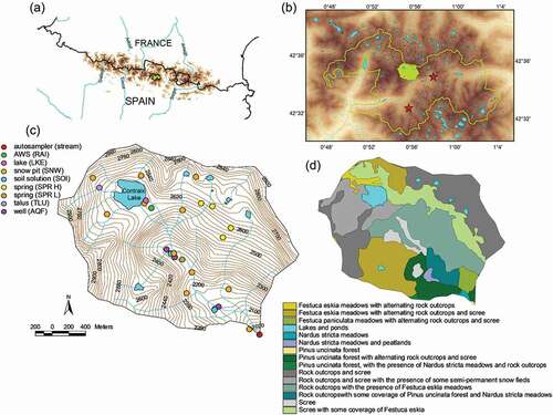
There are gradients in temperature and precipitation with elevation in the area, increasing from 7.7°C and 1241 mm/year at 1600 m a.s.l. to 1.6°C and 1515 mm/year at 2600 m a.s.l., respectively; therefore, the temperature and precipitation lapse rates are 0.62°C/100 m and 29.8/100 m, respectively. The year of study (2010) was 1.2°C colder than average, but precipitation was very similar to the average at both 1600 and 2600 m a.s.l. The temperature and precipitation data are the average values for 2010–2018 from our own automatic weather stations (AWSs).

Methodology

Sampling strategy

A sampling network was established across the Contraix catchment (Fig. 1(d)). An automatic sampling system was used to sample stream water, which was undertaken at a high frequency when storms and flow fluctuations occurred. The autosampler was placed near the outlet of the Contraix catchment and was used from March to November 2010, which covers the melting season (spring), when the flow is maximum, and summer and autumn, when the surface flow tends to stabilize and floods are caused by rainfall episodes.

To complete the information needed to carry out the mixing modelling, we determined the characteristic chemical compositions of potential end members (EMs): atmospheric waters (rainwater and snowpack), lake water (surface storage), and groundwater (water table, aquifers, talus, and springs). These characteristic values were not measured in all cases during the same year. The aim was not to obtain the values of the potential EMs at a specific time, but rather to obtain representative general values; thus, they are estimates of typical values for application in mixing modelling, rather than inputs for a step-by-step reconstruction of stream chemistry. The resulting variability of the potential EM estimates was high, but with little or no overlap between them, allowing us to infer a set of theoretical EMs that must be proposed to model the surface flow composition (see the “End member identification” section).

Rainwater and snowpack water were sampled fortnightly and monthly, respectively, from March to November 2010 (during the snowmelt and snow-free periods). Water from the water table was sampled monthly from August 2017 to June 2018. Aquifer water from deep wells was sampled monthly from September to November 2018. Talus water was sampled in July of 2013. The lake was sampled during the ice-free period from July to November 2013. Springs were sampled between July and December of 2017.

Rainwater was sampled from AWSs. Snowpack samples were taken from several snow pits distributed across the catchment at different altitudes. Six shallow wells were installed in the water table (three in the central part and three in the lower part of the catchment). For the aquifer samples, three deep wells were drilled at different altitudes next to the shallow wells. The talus water is represented by a single sample taken at the outlet of a micro-catchment in the somital area of Contraix Valley feeding Contraix Lake. Five lake water samples were collected from the lake surface during the ice-free period. Finally, several springs were also sampled, five in the highest area and another at a lower altitude.

Meteorological data

Meteorological data were obtained from two AWSs: one located in the highest area of the basin near Contraix Lake (altitude of 2593 m a.s.l.), and another located in a lower area outside the basin (altitude of 1674 m a.s.l.) near Llebreta Lake (Fig. 1(b)). Both are AWSs were equipped with sensors for air temperature and relative humidity (HMP45AC, Vaisala), global radiation (CMP6, Kipp & Zonen), net radiation (NR Lite, Kipp & Zonen), photosynthetically active radiation (PAR) (SKP215S, Skye), and wind speed and direction (Wind Monitor, Young). They also included a raingauge (T200B, Geonor) and a data acquisition/recording system (CR1000, Campbell Scientific).

Stream sampling

Stream water samples were collected at sub-hourly frequencies, proportional to the fluctuations of the stream level (from 10 minutes in the rising limb of the hydrograph to eight hours in the receding limb), which allowed us to capture in detail the chemical changes derived from abrupt hydrological events, such as melting episodes and storms. Thus, we were able to assess and quantify the effective relevance of these events in the hydrochemical balance. The automatic sampling system consisted of a precipitation gauge (SBS500, Campbell Scientific) and a stream water level sensor (PDCR1830, Druck) connected to a data recorder/processor (CR800, Campbell Scientific). The processor was programmed to anticipate and track the evolution of floods from precipitation and water level measurements, and to activate the water sampler (3700FS, ISCO) at the required times during the flood and subsequent water level recession. In total, 271 samples were collected. For collection and storage of all water samples, 1 L polyethylene (PE) bottles previously cleaned with deionized water (Milli-Q, Waters) were used. Caution was taken at all times to avoid contamination, and latex gloves were worn during sample handling. The autosampler was located at an altitude of 1969 m a.s.l.

The discharge was calculated from water level data. The discharge was previously calibrated by measuring the average water velocity with a current meter (GlobalWater) and multiplying it by the area of the section of the gauged stream at different water levels.

Atmospheric water sampling

Rainwater

To sample rainwater, two rain collectors were installed, one in each AWS. The rain collectors consisted of a 25 cm diameter PE funnel placed 1.5 m above the ground, which was connected to a 30 L sealed PE tank by means of a tube holding a 200 µm filter to prevent particles from entering the sample container. In total, 26 samples were collected.

Snowpack

Snowpack sampling was conducted following the methodology described by Bacardit and Camarero (2010). This involved digging a snow pit and sampling the shaded face of the pit. Subsamples from each snow layer were collected every 10 cm using a clean cube-shaped polyvinyl chloride (PVC) tool of 1 L volume. They were then mixed and stored in a clean PE bag to give an integrated snow profile sample. Snow samples were taken only after the first 20 cm of exposed snow from the sampled face was removed to avoid contamination. Sampling tools were carefully cleaned before use, and gloves were worn during sampling and handling to avoid sample contamination.

The samples were kept frozen until laboratory analysis. For analysis, they were allowed to melt completely at room temperature (~20°C) in their sampling bags. After melting, the samples were immediately filtered through glass fibre filters (Whatman, GF/F 47 mm diameter) and kept in a refrigerator until analysis.

A total of 16 samples (i.e. 16 snow profiles) were collected from the 10 points shown in Fig. 1(d). The sampling points were located at several altitudes between 2017 m and 2719 m a.s.l.

Groundwater sampling

Here, we distinguish between shallow groundwater, which encompasses water from the water table, talus water, and lower spring water, and deep groundwater, which encompasses aquifer water and high spring water.

Water table

For the sampling of the water table in the soil saturated zone, six shallow wells were installed, three in the middle part (2284 m a.s.l.) and another three in the lower part (2139 m a.s.l.) of the Contraix catchment. Those at higher altitudes had a depth of approximately 90 cm, while the three at lower altitudes had depths of 30–40 cm.

The wells had a diameter of 9 cm and were fitted with a sleeve consisting of a perforated PVC pipe to allow water to enter the well. This water was sampled with the help of a tube connected to a syringe with a three-way valve to alternate between suction from the well and drawing out to the sample bottle. A total of 46 samples were collected.

Talus water

Only one representative grab sample was collected at the outlet of a micro-catchment in the valley’s somital area where a small stream was forming. At the time of sampling, the area was composed exclusively of scree, with no vegetation.

Aquifer water

Three relatively deep wells were drilled in August 2018 (close to where the shallow wells were located) to extract water from different aquifers representative of the catchment’s deep groundwater (Fig. 1(d)). Previously, an electrical resistivity tomography (ERT) survey was conducted to locate aquifers. Two of the wells were located in the middle part of the catchment at depths of 14 m (well 1: 2296 m a.s.l.) and 10 m (well 2: 2284 m a.s.l.). The third well was located in the lower part of the catchment at a depth of 2 m (well 3: 2138 m a.s.l.).

The wells were lined with a ribbed screen PVC pipe that was capped at the top to prevent any material from entering. At the time of sampling, the pipe was uncovered, and a pump (2” Envirotecnics Super Twister submersible pump) connected to a narrow PVC tube was introduced. The pump was powered by conventional lead-acid batteries. Ten samples were obtained.

At higher altitudes (> 2600 m a.s.l.), the ERT survey did not provide any clear evidence of the presence of aquifers. Because of the uncertain results, and given the difficulties of drilling in this high-altitude terrain, a survey was conducted in search of springs as an alternative to sampling groundwater at these altitudes (Fig. 1(d)).

Spring water

A total of 13 grab samples were collected from four springs at high altitude in bare rock areas, where water emerged directly from the rock. This water was assumed to be representative of groundwater from the highest area of the catchment (i.e. > 2600 m a.s.l.). The altitudes of the four samples were 2650, 2625, 2604, and 2533 m a.s.l., respectively. Another spring was sampled at a lower altitude (2265 m a.s.l.), where soil was present. The two types of springs are hereafter referred to as “high” and “low” springs, respectively.

Lake water

Five grab samples of lake water were collected during the ice-free season from the shore of Lake Contraix and near the outlet, which is usually underground.

Laboratory analysis

Water samples for dissolved species analysis were filtered through pre-combusted (five hours at 450°C) glass fibre filters (GF/F, Whatman). Conductivity, alkalinity, and pH were measured upon arrival at the laboratory. Conductivity was measured using a WTW ProfiLine Cond 3310 instrument. Alkalinity was determined using automated Gran titration. For pH measurement, water samples were collected in bottles without air space and measured with an Orion Star A211 pH meter equipped with a fast response, low ionic strength electrode (Crison-Hach 5224 model) to avoid any gas exchange that could change the in situ pH value. Dissolved organic carbon (DOC) was measured by catalytic combustion and DIC was measured by acidification, and infrared spectrometry (Shimadzu TOC-5000 analyser) was then used to detect the produced CO₂. The major cations (Na⁺, K⁺, Ca²⁺, and Mg²⁺) and anions (Cl⁻, SO₄²⁻, and NO₃⁻) were measured by capillary electrophoresis using a Waters Quanta 4000 analyser. Ammonium (NH₄⁺), nitrite (NO₂⁻), and dissolved reactive silica (DRSi) were analysed using a segmented flow autoanalyser (AA3HR, Seal/Bran+Luebbe) and automated versions of the blue indophenol method (Berthelot reaction) (B + L G-171-96 method) for NH₄⁺, the Griess reaction (B + L G-173-96 method) for NO₂⁻, and the reduction of molybdosilicate to heteropoly blue (B + L G-171-96 method) for DRSi (Solozano 1969, Grasshoff 1983).

EMMA

Based on the concept that stream water can be defined as a mixture of different waters (i.e. EMs), EMMA can be used to identify and quantify the contributions of diverse hydrological compartments to surface flow. To quantify the contribution of each EM to the surface flow, the method relies on the use of conservative solutes that can serve as tracers for each EM (Christophersen et al. 1990, Christophersen and Hooper 1992). To apply this methodology, the number of EMs and their tracer solutes must be known.

In this study, prior to performing the EMMA, we applied a set of diagnostic tools (Hooper 2003) to determine the number of EMs involved in the model and their tracer solutes. First, a principal component analysis (PCA) was performed on the standardized results of the solute analysis of stream water samples. PCA is used to identify a small number of principal components (PCs) that substantially explain the chemical variability in a mixing space with fewer dimensions than those defined by the original variables. The variance explained by the subset of PCs must be highly significant (> 80% of the total variance) (Christophersen and Hooper 1992). For practical purposes, the number of PCs must be equal to or less than three; that is, the space defined by the PC subset has three dimensions at most.

In matricial terminology, PCA consists of finding an orthogonal matrix V containing PCs as rows such that

(1) $U=X^{\ast }\times V^T$(1)

where X* is the original standardized matrix of concentrations with dimensions n × s (n = number of samples; s = number of solutes), V^T is the transposed PC matrix with dimensions s × m (s = number of solutes; m = number of PCs), and U is the matrix of projected concentrations in the space defined by the PCs with dimensions n × m.

The concentrations of the solutes (X) were standardized using the mean (m) and standard deviation (SD) as follows:

(2) $X^{\ast }=\left(X-m\right)/sd$(2)

where X* is the standardized concentration.

In principle, PCA extracts as many PCs as solutes (i.e. m = s), but most of the variance in X* is captured by the first few PCs, and considering that only a few PCs are retained in the analysis (therefore m ≪ s), the resulting U is a subspace that has a much smaller dimension than X*.

Only conservative solutes can be used in EMMA as proper tracers of mixing. To check for conservativeness, a test is run on the residues (E), which are defined as the difference between the de-standardized solute concentration (X^{^}) for each sample as derived from its projection in the subspace U, and the original concentrations (X):

E = X^{^} – X(3)

De-standardized concentrations (X^) are calculated from their projection in U by computing the standardized concentrations (X*) using Equation (4):

(4) $X^{\ast }=U\times {\left(V\times V^T\right)}^{-1}\times V$(4)

and then de-standardized using Equation (5):

X^{^} = (X* × sd) + m(5)

For testing, the residues were plotted against the original concentrations. A lack of linear correlation (i.e. R² ≤ 0.1) between the residues and the observed solute concentrations indicates a random pattern in the residuals. A higher correlation suggests a deficiency in the mixing model that might arise from the violation of any of the assumptions in the mixing model, in particular from the non-conservative behaviour of solutes. Solutes that are found to be non-conservative must be removed from the analysis, and the PCA is performed again with the remaining solutes.

At the end of this iterative process, only the PCs that individually explain a proportion of the total variance greater than the value obtained by dividing 1 by the number of total components of the PCA is retained. The number of EMs needed is then equal to the number of retained PCs plus 1.

The next step was to build the mixing diagrams. Potential EMs were represented, together with all the stream samples, in a graph representing subspace U. To be truly possible EMs, the candidates should be a vertex of an envelope enclosing all stream samples.

Once EMs were identified, the contribution of each EM to the streamflow at each time (i.e. for each sample) was calculated using a system of equations. The number of equations depended on the number of unknowns (i.e. the number of EMs). For each stream sample j, a set of i equations (i = number of PCs) had to be solved in the form:

(6) $C_{i,j}=fE{M}_{k,j}\times E{M}_{k,i}+fE{M}_{k+1,j+1}\times E{M}_{k+1}{,}_{i+1}$(6)

where C_i,j is the PCA score of solute i for stream sample j; f EM_k,j is the fraction of EM_k in stream sample j; EM_k,i is the PCA score of solute i for EM_{k, i} = 1 to the number of PCs (m); j = 1 to the number of samples (n); k = 1 to the number of EMs (m + 1); and f EM_k,j is unknown, but its sum must be 1. This is the last equation required to complete the system:

(7) $1=fE{M}_{k,j}+fE{M}_{k+1}{,}_j$(7)

In matricial terminology, this system can be expressed as:

(8) ${U^T}^{,}=E\times F\hspace{0.17em}$(8)

where U^T’ is the transposed U matrix with an added row filled with 1s (and therefore dimension (m + 1) × n); E is the matrix with the PCA scores of each EM as columns plus a row filled with 1s (dimension (m + 1) × (m + 1)); and F is the unknown matrix ((m + 1) × n). This can be solved (with fractions converted to percentages) by computing:

(9) $F=E^{-1}\times {U^T}^{\prime }\hspace{0.17em}\times 100$(9)

These relative values were converted into absolute values (discharge in L s⁻¹) using the total discharge measurements.

Statistics

The PCA was conducted using the Rstudio software (version 1.1.463) with the command prcomp. The Excel Office (Microsoft) package (version 2016) was used for the EMMA calculations. Graphs were drawn using Sigmaplot (Insightful Inc.) software (version 14.0). The relationship between the stream water level (as a proxy of discharge) and the solute concentration was explored using the nonlinear regression command of the Sigmaplot software package. The level and concentration values were fitted to a power equation with two parameters (a and b):

(10) $Y=a{x}^b$(10)

where x is the stream level and Y is the solute concentration of interest. The adjusted R² value indicates goodness of fit, and significance was assessed on the basis of the p values of the individual parameter estimation.

Results

Chemical characteristics of each potential EM

The different types of water presented characteristic chemical features (Fig. 2). Compared with the other types of water analysed, snow water was the most dilute (low ion concentrations) and most acidic water. Rainwater was also relatively dilute. An outstanding feature of the rainwater samples was the high NH₄⁺ concentration. The level of DRSi was undetectable in both rainwater and snow water. The talus water sample was also relatively dilute, but with slightly higher concentrations of major cations (mostly Ca⁺, Na⁺, and Mg⁺) and DRSi. The lake water samples contained low cation concentrations, but presented relatively high concentrations of NO₂⁻ and DRSi.

Figure 2. Box-and-whisker plots of each of the solutes in the different water types. The first graph shows the number of samples for each water type

The similarity between stream water and the “high” spring water was remarkable. The only noticeable difference was the higher DIC concentration in the high spring water samples. Both were intermediate with respect to the concentrations of base cations and DRSi.

The “low” spring water was clearly different from the “high” spring water. Compared with the high spring samples, the low spring samples presented generally higher solute concentrations and considerably higher DIC and DOC concentrations. However, the NO₃⁻ concentration of the high spring samples was higher than that of the low spring samples.

The water table samples showed high concentrations of base cations and DIC but low NO₃⁻ concentrations. The aquifer samples had high concentrations of base cations, DRSi, and DIC. Compared with the water table samples, the aquifer samples had lower DOC concentrations and higher NO₃⁻ concentrations.

Stream water chemistry

The highest stream level was recorded during the thaw period (Fig. 3), from April to mid-June, although there were also significant increases in the streamflow after the snowmelt associated with intense rainfall, especially those events recorded in July.

Figure 3. Discharge and precipitation in the Contraix catchment during the study period

When comparing the concentration of each solute with the discharge level, a general dilution effect was observed when the river flow peaked. The plots of solute concentrations vs. discharge exhibited a negative exponential fit for most solutes, with an R² ranging from 0.55 (Mg²⁺) to 0.88 (for conductivity) (mean R² value of 0.75; Fig. 4). Only DOC, K⁺, and NH₄⁺ showed weak correlations, with R² values of 0.27, 0.21, and 0.39, respectively.

Figure 4. Streamflow vs. solute concentrations. The exponential curve fit and corresponding correlation value are shown. Thaw samples (26 March to 1 August) are shown in grey

EMMA results

Principal component analysis

The solute concentrations that were correlated with the residue (R² ≥ 0.1) were removed from the analysis. After the selection, only four solutes (Na⁺, Ca⁺, DOC, and DRSi) were used in the PCA. Two PCs were required to explain 95% of the total variance (Table 1), which was a sufficient fraction for our purposes (Christophersen and Hooper 1992). Therefore, at least three EMs were required to model the chemistry of the surface flow data. The results showed that PC1 was positively correlated with solutes derived from rock weathering (Ca²⁺, Na⁺, and DRSi), while PC2 was negatively correlated with DOC.

Table 1. Cumulative variance and loadings of the solutes in each PC based on PCA

	PC1	PC2
Ca	0.5755	−0.0101
Na	0.5723	0.1042
DRSi	0.5549	0.2224
DOC	0.1828	−0.9693
Accumulated variance	71%	95%

Mixing diagrams

Mixing diagrams were constructed in the space defined by the first two PCs (Fig. 5). Stream samples had to be within the two-dimensional envelope defined by at least three EMs to be a mixture of them. The potential EMs considered here were aquifer (AQF), snow (SNW), lake (LKE), rainwater (RAI), upper saturation zone (WTA), talus (TLU), high spring (SPR-H), and low spring (SPR-L) EMs.

Figure 5. Projection in the two-dimensional space presenting all stream samples, together with the average values of the a priori considered potential end members. Error bars are the standard deviations. Triangles represent the positions of the final proposed end members

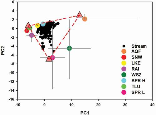
The SNW and RAI potential EMs were very similar. Both plotted on the left or negative side of PC1, and around zero on the axis defined by PC2 (Fig. 5). These EMs were characterized by very low solute concentrations, especially those originating from weathering. The SPR-H potential EM had a slightly positive value (but close to zero) on axes PC1 and PC2, and was characterized by intermediate solute concentrations, whereas the DOC concentration was near zero. The SPR-L potential EM was located on the slightly positive side of the PC1 axis, but with negative values on the PC2 axis, indicating moderately high Na⁺, Ca⁺, and DRSi concentrations and a high DOC concentration. The AQF potential EM plotted in the upper and right corners (Fig. 5, highest values of both PC1 and PC2), and was characterized by the highest concentrations of Na⁺, Ca⁺, and DRSi. The WTA potential EM plotted in an intermediate position between the SPR-L and AQF EMs, with positive values for PC1 and negative values for PC2 as a result of the high concentrations of Na⁺, Ca⁺, DRSi (although lower than those of the AQF EM), and DOC (similar to the SPR-L EM). The LKE and TLU potential EMs were chemically similar and plotted next to each other, slightly on the positive sides of the PC1 and PC2 axes. They were characteristically very dilute waters, with low concentrations of all solutes (although the LKE EM had somewhat higher concentrations). The TLU potential EM was most similar to the RAI potential EM.

End member identification

We inferred three empirical EMs that explained the chemical variability of the stream, as well as the composition of other a priori potential EMs: atmospheric water (ATM), deep groundwater (DGW), and shallow groundwater (SGW) EMs (Fig. 5). We situated them in the graph as the vertices of a triangle enclosing all stream samples, using the measured potential EMs as a guide. Therefore, the final EMs were as close as possible to the measured average of some potential EMs, and always within the uncertainty interval of one standard deviation (represented in Fig. 5 as error bars). The ATM EM included the RAI and SNW potential EMs, and plotted in the negative part of the PC1 axis (PC1 < 0) and around zero of PC2 (PC2 ≈ 0). The DGW EM plotted in the upper right-hand corner (PC1 > 0, PC2 ≈ 0), and was interpreted as the deep groundwater of the AQF potential EM. The SGW EM plotted in the lowest corner (PC1 ≈ 0, PC2 < 0), and included the WTA and SPR-L potential EMs. The variability of the WTA and SPR-L potential EMs was large (as shown by the error bars in the graph), with a substantial overlap. The SGW EM was parameterized to enclose the stream samples while still falling within the variability space of the shallow groundwater components.

The main features of the three inferred EMs were as follows (Table 2). The ATM EM was the most dilute water type, the DGW EM presented the highest concentrations of base cations derived from weathering, and the SGW EM had high concentrations of all solutes and a very high DOC concentration.

Table 2. Mean solute concentrations of each EM

Solute/water	ATM	DGW	SGW
Na (µeq L^−1)	0	68	22
Ca (µeq L^−1)	6	253	108
DOC (ppm)	0	1	5
DRSi (µeq L^−1)	14	132	42

Mixing model: contribution of each EM to streamflow

The ATM EM was the major contributor (average of 55%) to the surface flow during the entire time series (Fig. 6). The highest contribution (the maximum value for a single sample) was 70%, which occurred during the thaw period, and the lowest value (the minimum value for a single sample) was 5%, which occurred at the beginning of September.

Figure 6. Relative (upper panel) and absolute (lower panel) contributions of each end member to the streamflow over time

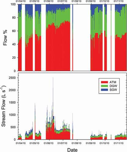
The average contribution of the DGW EM to the surface flow was 25%. The lowest values (5%) were observed during June and July, and the highest values (45%) were observed at the end of April and the beginning of September.

The average contribution of the SGW EM to the streamflow was 20%. The lowest values (4%) were observed in November. The contribution was uniform in other months, except for some episodes coinciding with rainfall events, when it reached 70%. These mostly occurred at the end of July and the beginning of September, although a couple of rainfall events were recorded in May and June.

Discussion

The rainwater samples were very dilute and had relatively high NH₄⁺ concentrations in comparison to the other water types. Although it is possible that the NH₄⁺ concentration in runoff water decreased as a result of nitrification in the catchment (Li et al. 1992), this would have involved an increase in the NO₃⁻ concentration, which was not observed. Thus, it is possible that there was also a consumption of NO₃⁻ in the catchment due to denitrification and plant assimilation (Bernal et al. 2006). A coupling of these two processes in space and time can be concluded in this type of catchment (Vila-Costa et al. 2014). As a result of these changes, the nitrogen forms were non-conservative and could not be used as tracers in the mixing model.

The water table and low spring samples presented relatively high DOC concentrations. This similarity occurred because the low spring is located in an area of significant soil coverage. The spring water likely received leachate/DOC from the soil it crossed. In addition, the DIC concentration was much higher than that expected based on its alkalinity, indicating the presence of CO₂, most likely due to microbial respiration in soil (Marx et al. 2017). High concentrations of base cations were also observed in the water table and deep well samples, thus agreeing with the results of Katz (1989) and indicating a relatively long retention time in the subsoil. Mineral weathering proceeds in the subsoil, and may be enhanced by the high availability of free acidity from CO₂. Relatively long residence times favour the accumulation of weathered solutes in underground water (Li et al. 2005). Despite its high concentration, DIC is not a good tracer of water from the water table because it is non-conservative; water in the upper saturation zone is oversaturated with respect to CO₂, and when it reaches the surface, most CO₂ is degassed. Although DOC can be biologically consumed (primarily as a source of carbon in heterotrophic respiration), the large amount present in the water from the water table is not exhausted. In addition, refractory forms of DOC may be present in high proportions. A high DOC concentration was an exclusive feature of the water table with respect to the other EMs, making DOC a good tracer of water from the water table (the upper saturation zone heavily influenced by soil) to be used in mixing modelling.

The stream level (used here as a proxy for discharge) showed a rapid, direct response to precipitation. The base cation concentration was expected to decrease under high precipitation due to the dilution effect (Broshears 1993). This was the case for Na⁺ and Ca²⁺, but not for K⁺ and Mg²⁺, which are usually found at low concentrations (K⁺ in particular is often close to the analytical detection level). Any significant dynamics of K⁺ and Mg²⁺ were probably masked or embedded within the analytical error.

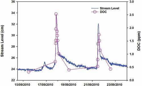
The concentrations of NH₄⁺ and DOC did not show a dilution effect at any stream level. The NH₄⁺ concentration was high in rainwater samples but was very low in the stream water samples. Considering that NH₄⁺ is rapidly oxidized by microbiota to obtain energy once it is deposited, it is possible to at least partially explain the non-dilutive behaviour by the precipitation contribution during high stream levels following storms. In the case of DOC, it is likely that water with a high DOC concentration stored in the water table was mobilized during storms and delivered to the stream (Hornberger et al. 1994, Boyer et al. 1997) (Fig. 7). The DRSi concentration of the water table samples was also relatively high; however, in contrast to DOC, it did not increase in the stream during floods. This apparent paradox can be explained by the fact that water samples from the water table had the highest DOC concentration, but the DRSi concentration was only slightly higher than that of the stream water samples. This could be explained by the effective dilution of aquifer water during storm floods (Buffam et al. 2001) under an increasing water table. The same was observed for Na⁺ and Ca²⁺.

Figure 7. Discharge and DOC concentration in the stream during two rainfall episodes, on 14 and 24 September 2010

Both EMMA and Hooper’s diagnostic tools were useful for carrying out mixing modelling in our catchment. This method has been applied here for the first time in the Pyrenees. Solutes such as K⁺, Mg²⁺, Cl⁻, and SO₄²⁻, that could be expected to behave conservatively, were found to be non-conservative; therefore, they could not be used for the mixing model (Gupta and Naik 1981). The non-conservative behaviour of K⁺, Mg²⁺, and Cl⁻ may relate to the fact that they were probably affected by ion exchange processes in the soil (Hendershot et al. 1993). This is especially significant because they were present at low concentrations. For SO₄²⁻, sulphate reduction probably played an important role. Similarly, N compounds may have been affected by biological reactions, such as nitrification, denitrification, and uptake. These biological processes cause changes in the concentrations of these solutes in a non-conservative manner (Postgate 1979).

Another important point is that EMMA could be applied without explicit knowledge of the EMs. In the absence of this knowledge, the methodology allowed us to infer the number of EMs and helped to identify them (Barthold et al. 2011). This last task was difficult because of the high variability (as reflected by the error bars in Fig. 5) with which EM candidates were presented. The requirement for an EM in EMMA is that it must be relatively constant over time. The use of PCA to construct a mixing space with a reduced dimension allowed us to clearly segregate (i.e. without overlapping of their respective variation) the candidate EMs and propose three functional EMs (ATM, SGW, and DGW) for modelling.

The catchment studied here is hydrologically dominated by meltwater along with the related processes and storms. Therefore, the contribution of atmospheric water throughout the year is expected to be dominant. However, the EMMA results indicated that, although large (55%), this contribution was quantitatively less than expected, especially outside the snowmelt period (although also within it at some particular moments).

It was remarkable how the volume of shallow groundwater increased, in both relative and absolute terms, during rainfall events that occurred during and after the late thaw period. This behaviour can be explained by the hydrological disconnection of soil (the unsaturated zone of soils in particular) during dry periods between precipitation (Torres et al. 1998). During these periods, soil probably accumulated solutes (e.g. DOC) that were then leached abruptly after a rainfall event (Fig. 7) by means of translational and lateral flow due to displacement caused by the entry of new water into the underground catchment (Cowie et al. 2017). This either did not occur or was less evident during the early thaw period because the continuous flow of water would have prevented the accumulation of solutes (Hoorman et al. 2011).

Another remarkable aspect was the continuous and almost regular contribution of the DGW EM over time, suggesting that deep groundwater in this type of mountain catchment could be an important factor contributing to the flow of headwater streams (Williams et al. 2006). This conclusion also has intrinsic implications for the future, considering that if climate change forecasts are met in these high mountain areas, the periods of snowfall and snow cover will decrease (Rangwala and Miller 2012), with changes in the timing of snowmelt as well. According to our results, this could have a deep impact on the chemistry of stream water, as snowmelt water is a key factor in aquifer recharge.

There is an extensive literature reporting studies that have used mixing models in many locations. However, studies in alpine catchments are much fewer in number. Cowie et al. (2017) provided in their table 1 a review of works that had applied EMMA in alpine, sub-alpine, and montane areas. Alpine areas included the Himalayas, the Rocky Mountains, and the Cordillera Blanca of Peru. Here we complete the review by including more recent studies conducted in alpine catchments. These studies have been conducted in Tibet, the Alps, and the Rocky Mountains. Our study adds the Pyrenees to the list of studied sites, for the first time. These new studies generally show more intensive data collection than the previous ones, with a sampling scheme more comparable to ours. Studies in Tibet (Jin-Kui et al. 2016) and the Alps (Rahman et al. 2015) have been carried out in catchments dominated by glacier hydrology. The EMs involved in these works were glacier meltwater, precipitation (or quick-routed surface runoff, as it was termed by Rahman et al. 2015), and groundwater (or slow-routed groundwater according to Rahman et al. 2015). These works have not considered soil water or shallow groundwater as a potential EM differentiated from groundwater. This is a contrasting result with respect to ours. We see a clear difference between deep and shallow groundwater. In any case, in these glacier-dominated catchments precipitation and groundwater had a minor weight compared to the glacier meltwater EM, which has a major effect all year round.

In the catchments studied in the Rocky Mountains (Cowie et al. 2017, Foks et al. 2018) there are no large glaciers, and they are therefore more similar to ours. Foks et al. (2018) defined four EMs – talus groundwater, soil water, rain and snow – whereas Cowie et al. (2017) identified only three Ems – groundwater, talus groundwater, and snow. The main discrepancies (including with our own results) are the number of EMs, the distinction between snow and rain made by Foks et al. (2018), and the absence of soil or shallow groundwater and rain as EMs in Cowie et al. (2017). Foks et al. (2018) differentiated rain and snow water by means of their ¹⁸O signature. We were not able to make such a distinction as we did not analyse ¹⁸O. Their EMs were otherwise comparable to our three EMs: deep groundwater (talus), shallow groundwater (soil), and atmospheric water (rain and snow).

The fact that soil water was not a significant EM in Cowie et al.’s (2017) study, in contrast to Foks et al.’s (2018) and ours, is more remarkable. This could be related to the sampling methods. In principle, our shallow groundwater should be more comparable to Cowie’s et al. (2017) soil water. In both cases it was water from the saturated zone of soil, sampled from either shallow wells (in our case) or zero-tension lysimeters, whereas Foks et al. (2018) used suction lysimeters able to also sample water from unsaturated soil. The opposite result in the two studies in the Rocky Mountains could be explained by a different chemistry of water from the saturated and unsaturated zones. On the other hand, a possible explanation for the disagreement between Cowie’s et al. (2017) study and ours is that, despite the fact that in both cases the samples are from the saturated zone, the sampling timing was different: Cowie et al. (2017) used a periodic, weekly sampling, whereas we used a more intensive and variable (and quite unique among the published alpine catchment studies so far) sampling design using an autosampler, intended to capture in detail short flood episodes following storms. Shallow groundwater was an specially important contributor to stream flow during these flashing episodes, and this could be the reason why it appears as one of the major EMs in our case. All three recent studies (including ours) presented two similar results: the atmospheric component is more important during the melting period, and groundwater is of importance in the EMMA, being a compartment that influences markedly the composition of the stream flow hydrographs during all seasons.

Our findings of a high percentage (45%) of underground water (both shallow and deep groundwater) maintained in streamflow, which increased during stormflow conditions, are consistent with the so-called “old water” paradox (Kircher 2003). This can be seen in the fact that streamflow responded promptly to rainfall inputs (1–3 days based on the hydrograph recession curve), but fluctuations in passive tracers indicated that storm flow was mostly old water (several months to a year in age; Camarero et al. 2018). Therefore, the discharge peaks were mainly composed of groundwater, not rainwater.

Main conclusions

The results showed that Na⁺, Ca⁺, DRSi, and DOC were conservative solutes; therefore, they were suitable tracers for mixing modelling. In our mixing model, three types of water were identified as EMs (ATM, DGW, and SGW) that could explain the chemistry of the stream water through mixing. These EMs were characterized as follows:

• ATM EM: low concentrations of all solutes included in the mixing model;

• DGW EM: high concentration of all solutes except DOC;

• SGW EM: very high DOC concentrations and intermediate concentrations of all other solutes.

The infiltration of a large volume of water through soil and rock fissures into the groundwater compartment during the melting season and storms displaced the existing groundwater via translational and lateral flow. This caused an important (45%) year-round contribution of groundwater to the surface flow, with peaks reaching > 70% during storm flow periods. Our results add to the evidence provided by other studies that the hydrology of high mountain catchments is more complex than that of a “Teflon basin.”

Hooper’s diagnostic tools were particularly useful for applying EMMA to estimate the different EM contributions to streamflow in the studied high mountain catchment. This study demonstrates the applicability of mixing modelling in high mountain catchments, which can help us better understand the hydrological dynamics of high mountain catchments by accounting for the role of groundwater to more accurately understand and predict changes (both in quantity and quality) in surface flow due to water discharges from different compartments. Furthermore, this work can serve as a basis for future studies in the Pyrenees region that aim to better understand and apply concepts that have entered hydrological research over the last decade, such as the so-called “old water” paradox.

Acknowledgements

The authors thank the directors and staff of the Aigüestortes i Estany de Sant Maurici National Park for their help during the field work.

Disclosure statement

No potential conflict of interest was reported by the author(s).

Additional information

Funding

This study was financed by the OAPN – Spanish Ministry of Environment [ACOPLA project, ref. 011/2008], and the Spanish Ministry of Science and Innovation [TRANSFER project, ref. CGL2016-80124-C2-2-P; pre-doctoral grant FPI to DM, ref. BES-2017-082740].

References

- Ajami, H., and Schreiner-McGraw, A., 2019. Characterizing mountain system recharge processes from headwaters to groundwaters. In: AGUFM, San Francisco, California. (Mascone Center), H52F–07.
- Antolino, D.J., 2019. Groundwater/surface-water interactions along Ellerbe Creek in Durham, North Carolina, 2016–18. US Geological Survey. (No. 2019-5097) Mascone Center, San Francisco, California.
- Bacardit, M. and Camarero, L., 2010. Atmospherically deposited major and trace elements in the winter snowpack along a gradient of altitude in the Central Pyrenees: the seasonal record of long-range fluxes over SW Europe. Atmospheric Environment, 44 (4), 582–595. doi:https://doi.org/10.1016/j.atmosenv.2009.06.022.
- Barthold, F.K., et al., 2011. How many tracers do we need for end member mixing analysis (EMMA)? A sensitivity analysis. Water Resources Research, 47 (8). doi:https://doi.org/10.1029/2011WR010604.
- Bates, B.L., et al., 2011. Influence of groundwater flowpaths, residence times and nutrients on the extent of microbial methanogenesis in coal beds: Powder River Basin, USA. Chemical Geology, 284 (1–2), 45–61. doi:https://doi.org/10.1016/j.chemgeo.2011.02.004.
- Battarbee, R.W., et al., 2002. Climate variability and ecosystem dynamics of remote alpine and Arctic lakes: the MOLAR project. Journal of Paleolimnology, 28 (1), 1–6. doi:https://doi.org/10.1023/A:1020342316326.
- Bernal, S., Butturini, A., and Sabater, F., 2006. Inferring nitrate sources through end member mixing analysis in an intermittent Mediterranean stream. Biogeochemistry, 81 (3), 269–289. doi:https://doi.org/10.1007/s10533-006-9041-7.
- Boyer, E.W., et al., 1997. Response characteristics of DOC flushing in an alpine catchment. Hydrological Processes, 11 (12), 1635–1647. doi:https://doi.org/10.1002/(SICI)1099-1085(19971015)11:12<1635::AID-HYP494>3.0.CO;2-H.
- Broshears, R.E., 1993. Tracer-dilution experiments and solute-transport simulations for a mountain stream. Saint Kevin Gulch, CO: US Department of the Interior: US Geological Survey.
- Buffam, I., et al., 2001. A stormflow/baseflow comparison of dissolved organic matter concentrations and bioavailability in an Appalachian stream. Biogeochemistry, 53 (3), 269–306. doi:https://doi.org/10.1023/A:1010643432253.
- Camarero, L., et al., 2018. Uso de isótopos estables y radiactivos en seguimiento e investigaciones a largo plazo (LTER) de los ecosistemas acuáticos de los Parques Nacionales: resultados del proyecto ISÓTOPOS. In: Madrid, Organismo Autónomo de Parques Nacionales, ed. Proyectos de investigación en Parques Nacionales: 2012–2015. Serie: investigación en la red. Colección: naturaleza y Parques Nacionales (pp. 267–285) .
- Christophersen, N., et al., 1990. Modelling streamwater chemistry as a mixture of soilwater end-members. A step towards second-generation acidification models. Journal of Hydrology, 116 (1), 307–320. doi:https://doi.org/10.1016/0022-1694(90)90130-P.
- Christophersen, N. and Hooper, R.P., 1992. Multivariate analysis of stream water chemical data: the use of principal components analysis for the end-member mixing problem. Water Resources Research, 28 (1), 99–107. doi:https://doi.org/10.1029/91WR02518.
- Cowie, R.M., et al., 2017. Sources of streamflow along a headwater catchment elevational gradient. Journal of Hydrology, 549, 163–178. doi:https://doi.org/10.1016/j.jhydrol.2017.03.044.
- De Jong, C., Collins, D.N., and Ranzi, R., 2005. Climate and hydrology of mountain areas. John Wiley & Sons ed.
- Engel, M., et al., 2016. Identifying run-off contributions during melt-induced run-off events in a glacierized alpine catchment. Hydrological Processes, 30 (3), 343–364. doi:https://doi.org/10.1002/hyp.10577.
- Fleckenstein, J.H., et al., 2010. Groundwater-surface water interactions: new methods and models to improve understanding of processes and dynamics. Advances in Water Resources, 33 (11), 1291–1295. doi:https://doi.org/10.1016/j.advwatres.2010.09.011.
- Foks, S.S., et al., 2018. Influence of climate on alpine stream chemistry and water sources. Hydrological Processes, 32 (13), 1993–2008. doi:https://doi.org/10.1002/hyp.13124.
- García-Ruiz, J.M., et al., 2010. From plot to regional scales: interactions of slope and catchment hydrological and geomorphic processes in the Spanish Pyrenees. Geomorphology, 120 (3–4), 248–257. doi:https://doi.org/10.1016/j.geomorph.2010.03.038.
- Grasshoff, P., 1983. Methods of seawater analysis. Verlag Chemie. FRG, 419, 61–72.
- Hazen, J.M., et al., 2002. Characterisation of acid mine drainage using a combination of hydrometric, chemical and isotopic analyses, Mary Murphy Mine, Colorado. Environmental Geochemistry and Health, 24 (1), 1–22. doi:https://doi.org/10.1023/A:1013956700322.
- Hendershot, W., et al., 1993. Ion exchange and exchangeable cations. Soil Sampling and Methods of Analysis, 19, 167–176.
- Hinckley, E.S., et al., 2014. Aspect control of water movement on hillslopes near the rain–snow transition of the Colorado Front Range. Hydrological Processes, 28 (1), 74–85. doi:https://doi.org/10.1002/hyp.9549.
- Hood, J.L. and Hayashi, M., 2015. Characterization of snowmelt flux and groundwater storage in an alpine headwater basin. Journal of Hydrology, 521, 482–497. doi:https://doi.org/10.1016/j.jhydrol.2014.12.041
- Hooper, R.P., 2003. Diagnostic tools for mixing models of stream water chemistry. Water Resources Research, 39 (3). doi:https://doi.org/10.1029/2002WR001528.
- Hoorman, J.J., et al., 2011. The biology of soil compaction. Soil Tillage Res, 68, 49–57.
- Hornberger, G., Bencala, K.E., and McKnight, D.M., 1994. Hydrological controls on dissolved organic carbon during snowmelt in the Snake River near Montezuma, Colorado. Biogeochemistry, 25 (3), 147–165. doi:https://doi.org/10.1007/BF00024390.
- Huggel C., et al., 2010. Recent and future warm extreme events and high-mountain slope stability. Philosophical Transactions of the Royal Society A: Mathematical, Physical and Engineering Sciences, 368 (1919), 2435–2459. doi:https://doi.org/10.1098/rsta.2010.0078.
- Huss, M., et al., 2010. Future high-mountain hydrology: a new parameterization of glacier retreat. Hydrology and Earth System Sciences, 14 (5), 815–829. doi:https://doi.org/10.5194/hess-14-815-2010.
- Jin-Kui, W., et al., 2016. Streamwater hydrograph separation in an alpine glacier area in the Qilian Mountains, northwestern China. Hydrological Sciences Journal, 61 (13), 2399–2410. doi:https://doi.org/10.1080/02626667.2015.1112393.
- Katz, B.G., 1989. Influence of mineral weathering reactions on the chemical composition of soil water, springs, and ground water, Catoctin Mountains, Maryland. Hydrological Processes, 3 (2), 185–202. doi:https://doi.org/10.1002/hyp.3360030207.
- Keller, F., Goyette, S., and Beniston, M., 2005. Sensitivity analysis of snow cover to climate change scenarios and their impact on plant habitats in alpine terrain. Climatic Change, 72 (3), 299–319. doi:https://doi.org/10.1007/s10584-005-5360-2.
- Kircher, J.W., 2003. A double paradox in catchment hydrology and geochemistry. Hydrological Processes, 17 (4), 871–874. doi:https://doi.org/10.1002/hyp.5108.
- Li, A.G., et al., 2005. Comparison of field and laboratory soil–water characteristic curves. Journal of Geotechnical and Geoenvironmental Engineering, 131 (9), 1176–1180. doi:https://doi.org/10.1061/(ASCE)1090-0241(2005)131:9(1176).
- Li, C., Frolking, S., and Frolking, T.A., 1992. A model of nitrous oxide evolution from soil driven by rainfall events: 1. Model structure and sensitivity. Journal of Geophysical Research: Atmospheres, 97 (D9), 9759–9776. doi:https://doi.org/10.1029/92JD00509.
- Liu, F., Williams, M.W., and Caine, N., 2004. Source waters and flow paths in an alpine catchment, Colorado Front Range, United States. Water Resources Research, 40 (9). doi:https://doi.org/10.1029/2004WR003076.
- López-Moreno, J., Goyette, S., and Beniston, M., 2009. Impact of climate change on snowpack in the Pyrenees: horizontal spatial variability and vertical gradients. Journal of Hydrology, 374 (3–4), 384–396. doi:https://doi.org/10.1016/j.jhydrol.2009.06.049.
- Marx, A., et al., 2017. A review of CO2 and associated carbon dynamics in headwater streams: a global perspective. Reviews of Geophysics, 55 (2), 560–585.
- Penna, D., et al., 2017. Response time and water origin in a steep nested catchment in the Italian Dolomites. Hydrological Processes, 31 (4), 768–782. doi:https://doi.org/10.1002/hyp.11050.
- Postgate, J.R., 1979. The sulphate-reducing bacteria. Cambridge: CUP Archive.
- Rahman, K., et al., 2015. Quantification of the daily dynamics of streamflow components in a small alpine watershed in Switzerland using end member mixing analysis. Environmental Earth Sciences, 74 (6), 4927–4937. doi:https://doi.org/10.1007/s12665-015-4505-5.
- Rangwala, I. and Miller, J.R., 2012. Climate change in mountains: a review of elevation-dependent warming and its possible causes. Climatic Change, 114 (3–4), 527–547. doi:https://doi.org/10.1007/s10584-012-0419-3.
- Rodriguez, M., et al., 2016. Estimating runoff from a glacierized catchment using natural tracers in the semi‐arid Andes Cordillera. Hydrological Processes, 30 (20), 3609–3626. doi:https://doi.org/10.1002/hyp.10973.
- Schmieder, J., et al., 2018. Spatio‐temporal tracer variability in the glacier melt end‐member—how does it affect hydrograph separation results? Hydrological Processes, 32 (12), 1828–1843. doi:https://doi.org/10.1002/hyp.11628.
- Solozano, L., 1969. DETERMINATION OF AMMONIA IN NATURAL WATERS BY THE PHENOLHYPOCHLORITE METHOD 1 1 This research was fully supported by US Atomic Energy Commission Contract No. ATS (11‐1) GEN 10, PA 20. Limnology and Oceanography, 14 (5), 799–801. doi:https://doi.org/10.4319/lo.1969.14.5.0799.
- Studies on calcium, magnesium & sulphate in the Mandovi & Zuari River systems (Goa). NISCAIR-CSIR, New Delhi, India.
- Torres, R., et al., 1998. Unsaturated zone processes and the hydrologic response of a steep, unchanneled catchment. Water Resources Research, 34 (8), 1865–1879. doi:https://doi.org/10.1029/98WR01140.
- Vila-Costa, M., et al., 2014. Nitrogen-cycling genes in epilithic biofilms of oligotrophic high-altitude lakes (Central Pyrenees, Spain). Microbial Ecology, 68 (1), 60–69. doi:https://doi.org/10.1007/s00248-014-0417-2.
- Viviroli, D., et al., 2011. Climate change and mountain water resources: overview and recommendations for research, management and policy. Hydrology and Earth System Sciences, 15 (2), 471–504. doi:https://doi.org/10.5194/hess-15-471-2011.
- Williams, M., et al., 2006. Geochemistry and source waters of rock glacier outflow, Colorado Front Range. Permafrost and Periglacial Processes, 17 (1), 13–33. doi:https://doi.org/10.1002/ppp.535.
- Williams, M.W., et al., 2015. The ‘teflon basin’myth: hydrology and hydrochemistry of a seasonally snow-covered catchment. Plant Ecology & Diversity, 8 (5–6), 639–661. doi:https://doi.org/10.1080/17550874.2015.1123318.
- Zuecco, G., et al., 2019. Understanding hydrological processes in glacierized catchments: evidence and implications of highly variable isotopic and electrical conductivity data. Hydrological Processes, 33 (5), 816–832.