Are moments of rainfall spatial variability useful for runoff modelling in operational hydrology?

ABSTRACT

Moments of rainfall spatial variability, which quantify how flood response time scales are affected when spatially variable rainfall is considered, compared to when rainfall is spatially uniform, have been suggested as a useful tool for forecasters to guide their choice between lumped or distributed rainfall information for runoff modelling. However, the approaches used to evaluate the validity of moments suffer from limitations. Hence, we adopt a novel approach for their evaluation by comparing moments to the relationship between observed hydrograph characteristics generated by spatially variable and by uniform rainfall events in the same catchment. We further investigate the usefulness of moments by testing whether the performance of a lumped hydrological model for events classified by moments as spatially variable is lower than for uniform events. Results confirmed that moments can identify spatially variable events and characterize differences in hydrograph features compared to uniform events, providing a useful tool for forecasters.

KEYWORDS:

• rainfall spatial variability
• spatial variability statistics
• localized events
• runoff modelling

Editor S. Archfield Associate Editor I. Prosdocimi

1 Introduction

The influence of rainfall spatial variability on the runoff response at the catchment scale has been widely studied in hydrology, especially with the growing availability of high-resolution rainfall products. However, runoff response is the result of complex interactions between hydrological inputs (e.g. rainfall), landscape properties (e.g. soil properties) and catchment properties and hence clear conclusions have not been reached yet. In fact, some studies have highlighted little or no improvement when spatially distributed rainfall information is taken into account compared to using catchment-averaged values (e.g. Obled et al. 1994, Bell and Moore 2000, Reed et al. 2004, Das et al. 2008). Others have shown improvements in streamflow estimates when the spatial rainfall information is considered (e.g. Singh 1997, Cole and Moore 2008, Bonnifait et al. 2009, Euser et al. 2015). The reasons for these contrasting conclusions remain unclear.

Exploring the influence of rainfall spatial variability on the runoff response is certainly useful for researchers, who can better understand the rainfall–runoff dynamics and develop model structures that account for the rainfall spatial variability. Nevertheless, the research question is also important for practitioners and forecasters, with providing answers for the latter being one of the primary goals of this work. By knowing under what conditions rainfall spatial variability matters for runoff response, forecasters can make a more informed choice on the use of lumped or distributed rainfall information, optimizing the computational times to produce hydrological forecasts (Emmanuel et al. 2017).

Due to the limited time to issue a forecast, practitioners generally look for simple and fast-running tools to spot “alarming” behaviour in the catchment response to rainfall. For example, in the context of flash floods they rely on products such as the European Precipitation Index (Alfieri and Thielen 2015), which is a rainfall-driven indicator to identify storms that can generate flash flooding, or on rainfall threshold approaches (Pilling et al. 2016, Sharpe and Cranston 2021). As suggested by Emmanuel et al. (2017), measures of rainfall spatial variability, which describe the storm pattern with respect to the catchment, could be similarly used by practitioners to identify a priori events for which rainfall spatial variability plays an important role in shaping the hydrograph. These measures, named spatial moments (Zoccatelli et al. 2011), quantify how time scales of flood response are affected when spatially variable rainfall is considered, compared to when rainfall is assumed to be spatially uniform.

Two approaches have previously been used to test whether the moments of rainfall spatial variability are successful in describing the storm pattern and hence the runoff response due to the rainfall spatial pattern: (1) checking for proportionality between the moments computed from “real-world” events and their mathematical expressions derived under specific hypotheses (see equations (11) and (13) and fig. 5 in Zoccatelli et al. 2011); and (2) checking for better modelling performance using distributed rainfall information compared to spatially lumped information for those events that are classified as spatially variable by the moments (e.g. Lobligeois et al. 2014). However, both approaches suffer from limitations, if moments are to be used in practical applications. In the first approach, the assumptions made to derive the analytical formulae (i.e. runoff coefficient uniform in space and time and negligible hillslope residence time) cannot always be verified and hence the validity of the relationship between moments and runoff response for real-world applications is unclear. The second approach relies on hydrological modelling, which requires many additional assumptions about model structure, parameter values and eventually other distributed forcing inputs for the case of distributed hydrological models. These assumptions can mask or enhance the role of rainfall spatial variability, generating uncertainty regarding the validity of the moments when using other hydrological model structures and inputs.

For this reason, in this work we will evaluate the moments of rainfall spatial variability using a direct comparison between measured characteristics of hydrographs generated by spatially variable events and by uniform events happening in the same catchment. In this work we will test whether it is possible to link the moments to simple characteristics of the hydrograph such as response time and runoff coefficient, reducing the number of assumptions needed. If we find the relationship between the moments and runoff response due to rainfall spatial pattern described in Zoccatelli et al. (2011), we can then assume that the moments are a reliable tool to identify events that show a runoff response longer/shorter or more/less peaked than the response for uniform events happening in the same catchments. In this way the spatial moments can help address the pragmatic question of when distributed rainfall information is more appropriate than lumped rainfall for reliable operational hydrological modelling.

The main novelty of this study lies in the approach presented in the paragraph above. To the best of our knowledge, this is the first study presenting the evaluation of moments through a direct comparison between measured characteristics of hydrographs generated by spatially variable events and by uniform events happening in the same catchment, reducing dramatically the number of a priori assumptions. The aim of this study is not necessarily to gain new hydrological insight, but to reduce uncertainty in existing knowledge using a more objective approach, which can confirm the appropriateness of moments for deciding between lumped or a distributed rainfall information for operational hydrological modelling.

The analysis is framed through three main questions: (1) How frequently and in what type of catchments do we observe spatially variable rainfall events in Great Britain? (2) Can moments of spatial rainfall variability predict a priori characteristics of the hydrographs caused by the spatially variable rainfall spatial pattern with respect to uniform events happening in the same catchment? (3) Do events classified as spatially variable by the spatial moments show a lower performance score compared to the ones classified as uniform, when simulated with a lumped hydrological model?

2 Methodology

2.1 Selection of hydrologically meaningful events

The focus of this work is to understand whether measures of rainfall spatial variability are able to provide a priori information about the corresponding hydrograph response. Hence, we first define the rainfall events and later associate the corresponding streamflow events, as the corresponding streamflow is assumed to be unknown when extracting information from the rainfall event. For rainfall event identification, we make use of the concept of minimum inter-event time (MIT), the duration of the minimum dry period to separate rainfall contribution into different events (Dunkerley 2008). Unlike examples found in the literature, here we suggest defining its value using a physically based approach. This allows a more hydrologically meaningful rainfall event selection. Since we want to delimit sections of the hyetograph that match the responses in the hydrograph, we set the MIT value equal to the catchment response time (Tr) (Giani et al. 2021). Although the response time can vary depending on different initial conditions and storm types, using a physical characteristic of the catchments would produce a more realistic selection of rainfall events compared to a constant duration of the minimum dry spell across different catchments (e.g. Asquith et al. 2005, Bracken et al. 2008). When setting the MIT equal to Tr we aim to mimic the fact that if the inter-event time is shorter than Tr, the rainfall contribution from two consecutive rainfall events will probably be part of the same hydrograph peak (Fig. 1, left); if, in contrast, we have two consecutive rainfall events where the inter-event time is longer than Tr, we will probably observe two different peaks in the hydrograph (Fig. 1, right).

Figure 1. Graphic representation of setting minimum inter-event time (MIT) equal to catchment response time.

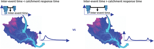
This methodology leads to a catchment-specific selection of rainfall events, longer in slower catchments and shorter in faster ones. The catchment is seen as an isolated system and therefore, for the same storm occurring over contiguous catchments, we can have a different event identification. In fact, the idea is to provide a methodology that groups rainfall contributions taking into account the response time of the catchment.

For the purpose of defining an appropriate value for the MIT, the Tr is estimated using the detrending moving-average cross-correlation analysis-based (DMCA) method applied to the entire rainfall and streamflow time series in each catchment (Giani et al. 2021). Unlike other methods available in the literature for estimating Tr (e.g. Grimaldi et al. 2012), the DMCA method is based on rainfall and streamflow hourly time series only and does not require event selection, hydrograph separation or parameter calibration (Giani et al. 2021). Hence, its estimate is more objective since it does not require any user decisions. In the case of flood forecasting, when the streamflow record is not yet available, the Tr estimate could be still retrieved with the DMCA method but using historical data.

The associated streamflow events are identified as follows: the beginning of the streamflow event is identified by the first point of increase in streamflow after the beginning of the rainfall event, and the end of the streamflow event is the last point before the streamflow starts rising again at the beginning of the following event. Moreover, two further conditions are applied when identifying events in order to guarantee a sensible selection of events: (1) peak discharge at least 1.5 times the pre-event discharge, as suggested by Norbiato et al. (2009) and by Graeff et al. (2012), to make sure there is a response in the streamflow record related to the identified rain event; (2) pre-event discharge lower than the 70^th percentile of the discharge distribution in each catchment, to reduce the influence of the antecedent event. The threshold for this last condition was arbitrarily chosen, but we checked that this value does not influence the overall findings of this work.

2.2 Describing rainfall spatial organization using moments of rainfall spatial variability

Rainfall spatial variability for each event is assessed by estimating first- and second-order rainfall moments (Zoccatelli et al. 2011, code available at https://github.com/giuliagiani/Moments_spatial_variability_of_rainfall). The moments are intended to quantify how time scales of flood response are affected when spatially variable rainfall is considered, compared to when rainfall is assumed to be spatially uniform. Moments of rainfall spatial variability can be computed either per time step or for the entire event by cumulating or averaging the rainfall over the duration of the rainfall event. In our case, we are interested in the impact of rainfall spatial variability at the event scale. However, to minimize the impact of the event duration on a moment’s value, we compute the moments using a time window equal to Tr of maximum rainfall for each of the identified events. In fact, longer rainfall events would tend to produce more uniform and centred distributions, as the rainfall has more chances to fall everywhere in the catchment. Note that we do not step back from the position of the runoff peak as suggested by Emmanuel et al. (2017) as we compute the spatial moments a priori, using the time window of maximum rainfall for each event.

According to the definition of Zoccatelli et al. (2011), the first moment D1 (see Equation A1 in the Appendix) “describes the distance of the centroid of the catchment rainfall with respect to the average value of flow distance (i.e. the catchment centroid) (p. 3769).” When D1 produces values larger than 1, the mean travel time with spatial rainfall is greater than the mean travel time with uniform rainfall (i.e. the centroid of the storm is located in the headwaters); when D1 produces values smaller than 1, the mean travel time with spatial rainfall is smaller than the mean travel time with uniform rainfall (i.e. the centroid of the storm is close to the catchment outlet); when D1 is equal to 1 the mean travel time with spatial rainfall is equal to the mean travel time with uniform rainfall (i.e. the centroid of the storm is located at the centroid of the catchment) (Fig. 2(a)).

Figure 2. Examples of rainfall distribution for (a) D1 and (b) D2 values greater than, equal to and lower than 1. Contour lines indicate distance to catchment outlet in metres. Colours represent the averaged rainfall over the window of maximum rainfall.

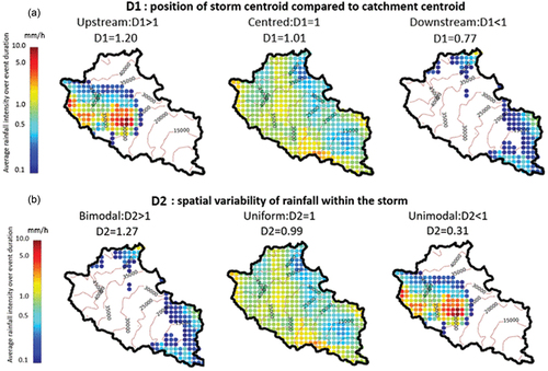
The second moment D2 (see Equation A2 in the Appendix) “describes the dispersion of the rainfall-weighted flow distances about their mean with the respect to the dispersion of flow distances” (Zoccatelli et al. 2011, p. 3769). When D2 assumes values larger than 1, the unit hydrograph is more spread out in time for spatially variable rain, compared to spatially uniform rain (i.e. flood hydrographs that are longer and less peaked or multi-peaked); when D2 assumes values smaller than 1, the unit hydrograph is more concentrated in time, compared to spatially uniform rain (i.e. rainfall is spatially concentrated somewhere in the basin); when D2 is equal to 1 the unit hydrograph is as concentrated in time as spatially uniform rain (Fig. 2(b)).

2.3 Benchmarking the performance of the moments of rainfall spatial variability with characteristics of the observed hydrograph

Firstly, the information content of the moments of rainfall spatial variability is investigated through a novel approach, a direct comparison between moment values and features of the observed hydrographs. The absence of hydrological modelling at this stage allows us to explore the influence of rainfall spatial variability without introducing any uncertainty related to the rainfall–runoff modelling process.

As mentioned in Section 2.2, the first moment, D1, describes the position of the storm centroid compared to the catchment centroid. According to Zoccatelli et al. (2011), D1 can be expressed as follows, under the hypothesis of a uniform runoff coefficient in space and time and negligible hillslope residence time (Equation 1(1) $D1=\frac{E\left(Tc\right)}{\frac{g1}{v}},$(1) ):

(1) $D1=\frac{E\left(Tc\right)}{\frac{g1}{v}},$(1)

where Tc is the time to route the rainfall excess from the geographical centroid of the rainfall spatial pattern to the catchment outlet, averaged by the operator E(*), and g1/v is the time to route the rainfall excess from the catchment centroid to the catchment outlet.

In this study we still use E(Tc), named here Tr_event, but we substitute the denominator g1/v, which corresponds to the response of centred events under the above hypothesis, with the response time of centred events in the same catchment, Tr_centred. For operational hydrologists it is more useful to have as a reference the “real-world” centred response time rather than a rigorously derived quantity under a more restrictive hypothesis.

As D1 describes the position of the storm centroid compared to the catchment centroid, we expect ratios (Tr_event/Tr_centred) larger than 1 when the centroid of the event is located upstream (D1 > 1), and ratios smaller than 1 when the centroid of the event is located downstream (D1 < 1).

The response of each event Tr_event is estimated using an adaption of the DMCA-based methodology on individual events (Giani et al. 2021, section 2.1.3). For the response time of centred events Tr_centred we should consider the Tr_events estimates for events with a D1 value close to 1 (i.e. centred events). Alternatively, if the majority of events show D1 values close 1, we can just compute Tr_centred as the median of the distribution of all the individual event response times for that catchment (we will show that this is indeed the case).

The second moment, D2, describes how uniform the storm is in space. According to Gaál et al. (2012, equation (13)), under the hypothesis of a uniform runoff coefficient in space and time and negligible hillslope residence time (Equation 2(2) $D2\sim Var\left(Tc\right),$(2) ):

(2) $D2\sim Var\left(Tc\right),$(2)

where Tc is the time to route the rainfall excess from the geographical centroid of the rainfall spatial pattern to the catchment outlet, and Var(*) is the variance operator. Var(Tc) is proportional to the square of the hydrograph duration. Hence, smaller values of Var(Tc) mean hydrographs with shorter durations and vice versa. For the same runoff depth, shorter duration will therefore generate higher peaks (Zoccatelli et al. 2011), which can be captured by the event peak runoff coefficient C_event as described by the rational formula (Kuichling 1889) (Equation 3):

(3) $C_{event=\frac{3.6Q_{peak}}{iA},}$(3)

where C_event is the dimensionless peak runoff coefficient of the event, Qpeak (m³/s) is the maximum streamflow for the event, i is the catchment average rainfall intensity (mm/h) for the window length equal to the time of concentration of maximum rainfall and A is the catchment area (km²).

Hence, in this work for each individual event we compare the D2 value against the ratio between the peak runoff coefficient of the individual event C_event and the peak runoff coefficient of uniformly distributed events in that catchment C_unif. We expect C_event/C_unif ratios higher than 1 when events are localized (D2 < 1 and potentially also D2 > 1 when also bimodal in time).

For the estimate of C_event, the use of time of concentration suggested by the rational formula (Kuichling 1889) is substituted with the Tr retrieved with the DMCA-based method (Giani et al. 2021), although we acknowledge this is conceptually slightly different (Beven 2020). For the peak runoff coefficient of uniformly distributed events C_unif we should consider in each catchment the C_event estimates of events with D2 value close to 1 (i.e. uniform events). Alternatively, if the majority of events in a catchment have mainly D2 values close to 1, C_unif can be computed as the median of all the individual event peak runoff coefficients for that catchment (we will show as this is indeed the case).

2.4 Benchmarking the skill of the moments of rainfall spatial variability using a lumped hydrological model

As a further test, the information content of the moments of rainfall spatial variability is investigated using a lumped hydrological model. The use of a distributed model was excluded a priori because the calibration process can be very complex and a poor calibration can mask the effect of spatial rainfall variability in shaping the hydrograph (Smith et al. 2004). When using a lumped model, in each catchment we expect to observe a lower model performance when the model is evaluated on events that have been classified by the moments as spatially variable. A higher performance score is expected for events that have been classified as uniform and centred, whereas applying a lumped model to spatial variable rainfall events will negatively impact the model performance, as by not capturing spatial variability the modelled streamflow will be altered. With this analysis, we aim to highlight for which events practitioners will need to improve their assessments by considering spatially distributed rainfall information, and that moments of rainfall spatial variability can help detecting those events.

The model structure used for this analysis is the probability distribution model (PDM; Moore 2007). It is a simple model with a probability-distributed soil moisture storage component, a surface storage component and a groundwater storage component. The model has been widely applied across the world for both design and operational purposes. It is also one of the most commonly used hydrological models in the UK, where our study catchments are located, and this guided our choice.

We perform a Monte Carlo simulation with 10 000 parameter sets to calibrate the PDM in each catchment using 50% of the available temporal record. The models are then used for continuous simulation on the other 50% of the data. Model evaluation is performed on all the identified events not involved in the calibration process, including both spatially variable and uniform events. We use the Kling-Gupta efficiency (KGE) score (Gupta et al. 2009) to evaluate the performance of the models in both calibration and evaluation. Among all the skill scores (Hall 2001, Dawson et al. 2007, Knoben et al. 2019), KGE was selected because it is widely used and accepted in the hydrological community. Furthermore, as the three components of the score can be assessed individually, this gives more insight into model performance (Equation 4(4) $KGE=1-\sqrt{{\left(r-1\right)}^2+{\left(\alpha -1\right)}^2+{\left(\beta -1\right)}^2},$(4) ):

(4) $KGE=1-\sqrt{{\left(r-1\right)}^2+{\left(\alpha -1\right)}^2+{\left(\beta -1\right)}^2},$(4)

where r is the linear correlation between observations and simulations; $\alpha$ is the ratio between σ_obs, the standard deviation in observations, and σ_sim, the standard deviation in simulations; and $\beta$ is the ratio between μ_sim, the simulation mean, and μ_obs, the observation mean. A perfect score for KGE is 1 (when r = 1, $\alpha$=1, $\beta$ =1), and any value larger than −0.41 can be interpreted as better than a simple average (Knoben et al. 2019).

3 Study catchments and data

The study catchments are part of the UK Benchmark Network 2 (UKBN2; Harrigan et al. 2018), a subset of catchments from the UK’s National River Flow Archive (NRFA) which have been classified as near-natural. The limited human disturbance in these catchments allows us to test the information content of moments of rainfall spatial variability without adding more complexity. The NRFA also provides a number of catchment descriptors, such as the baseflow index (BFI), which is used in the catchment selection to exclude those catchments which are highly baseflow dominated and show little response to rainfall.

It is usually accepted that a time step ranging between 20% and 50% of the Tr is suited to correctly represent the rising part of the hydrograph (Emmanuel et al. 2016). Hence, with hourly rainfall data, we only considered those catchments in the UKBN2 that have an average Tr greater than five hours. The Tr is estimated using the DMCA-based method on rainfall and streamflow time series (Giani et al. 2021). Moreover, the selected catchments have a BFI lower than 0.85, to guarantee a significant fast response in the hydrograph.

Continuous hourly rainfall on a 1 km grid with coverage over the whole of Great Britain for the time period 1990–2014 is provided by the Centre for Ecology and Hydrology gridded estimates of hourly areal rainfall for Great Britain (CEH-GEAR1hr) data product (Lewis et al. 2019). This product comes from the interpolation of over 1900 quality-controlled rainfall raingauges, providing an average coverage of one gauge in every grid cell of 10 × 10 km. To assess the spatial organization of rainfall, we also need flow distances to the catchment outlet of each point on the 1 km grid falling in the catchment area. Using the TopoToolbox 2 in Matlab (Schwanghart and Scherler 2014), flow distances have been computed starting from a digital elevation model at 50 m resolution, the UK NETMAP 50 m gridded Digital Elevation Model (Intermap Technologies 2009).

Streamflow data at a 15-min time step were provided for the same period, 1990–2014, or for a sub-period within this time interval, by the Environmental Agency (EA), Natural Resources Wales (NWR) and Scottish Environmental Protection Agency (SEPA) and then processed to obtain hourly streamflow time series. The dataset is visually checked for any anomalous records. The percentage of missing values in the available streamflow records can vary from 0 to 60% with a median value of 0.008%. We did not discard any of the catchments with higher percentages of missing values as we could still select events from the continuous parts of the records.

Potential evapotranspiration (PET) data based on the Penman-Monteith equation (Monteith 1965) are provided by the Centre of Ecology and Hydrology (CEH) at a daily scale (Robinson et al. 2016). We disaggregate this dataset at hourly resolution by first defining the length of the day according to the calendar year and the latitude of the catchment. Given that PET can be non-null only between sunrise and sunset, we use a probability density function scaled to the length of the considered day, and which preserves the total daily PET (Kumar et al. 2019). This procedure is repeated for each day in the original dataset.

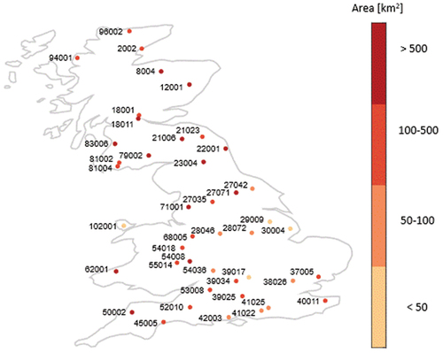
Considering the data availability and our own data requirements, the catchment study set consists of 43 out of 137 catchments that are part of UKBN2 (Fig. 3). We excluded catchments located in Northern Ireland because the considered rainfall product does not cover that area. Further sites were excluded if hourly streamflow data were not available or if Tr was less than five hours of BFI values above 0.85. The areas of the selected catchments range from 16 to 1508 km², with a median value of 285 km², and their lengths of record range between 17 and 24 years. The study catchments are nearly natural and hence mostly rural (permeable soils). The majority have a mean elevation between 50 and 150 m.a.s.l., with some reaching a mean elevation between 400 and 600 m.a.s.l. in the northern part of Great Britain. The study catchments are dominated by a wet climate with mainly stratiform events in winter and some thunderstorms in summer.

Figure 3. Catchment study set. The numbers indicate the catchment’s ID according to the UK Benchmark Network 2 (UKBN2) (Harrigan et al. 2018).

4 Results

4.1 How frequently and in what type of catchments do we observe spatially variable rainfall events in Great Britain?

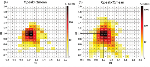
With our first question we would like to understand how frequently moments of rainfall spatial variability have values that indicate spatial patterns in storms. In Fig. 4 we present the distribution of the moment values, dividing the events into two groups. Figure 4(a) shows moment values for events that have a runoff peak larger than the mean streamflow value in the same catchment (calculated using the entire time series), while Fig. 4(b) shows moment values for events smaller than the mean streamflow values. Both figures show a bell shape slightly shifted towards upstream events. Bimodal events seem rarer than unimodal events and are usually characterized by a storm centroid located close to the catchment centroid. However, the majority of events are concentrated around D1 = 1 and D2 = 1, meaning they are centred and uniform. Larger events Fig. 4(a) show even less spatial variability, meaning that when larger events occur the storm is uniformly covering the catchment area.

Figure 4. Moments of rainfall spatial variability values and density for events (a) larger and (b) smaller than the mean streamflow value.

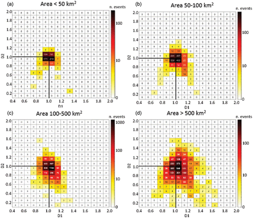
When organizing the moment values by catchment size (Fig. 5), we can see, as expected, that the majority of spatially variable events occur in larger catchments. In particular we can see how in moving from smaller to larger areas the number of more variable events increases, with the largest variability in catchments larger than 500 km² (Fig. 5(d)).

Figure 5. Moments of rainfall spatial variability values and density by catchment size: (a) < 50 km², (b) 50–100 km², (c) 100–500 km², (d) > 500 km².

4.2 Is there any relationship between moments of rainfall spatial variability and characteristics of observed hydrographs?

A comparison of D1 values versus event response time is presented in Fig. 6(a) (all events), 6(b) (events larger than the mean flow) and 6(c) (events smaller than the mean flow), while a comparison of D2 values versus runoff coefficient is presented in Fig. 6(d) (all events), 6(e) (events larger than the mean flow) and 6(f) (events smaller than the mean flow). The grey horizontal line in Fig. 6(a–c) represents Tr_event equal to Tr_centred (computed as the median of events of all magnitudes in each catchment), while in Fig. 6(d–f) it represents C_event equal to C_unif (computed as the median of events of all magnitudes in each catchment).

Figure 6. Comparison between D1 and response time, and D2 and runoff coefficient considering all events (a, d), events larger than the mean flow (b, e), and events smaller than the mean flow (c, f). The grey horizontal line represents the Tr_centred computed on events of all magnitudes for (a–c), and the C_unif computed on events of all magnitudes for (d–f). At the top of each box plot we show the sample size for each bin.

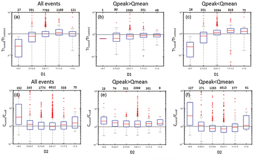
The relationship between D1 and response time seems weak in Fig. 6(a), but it appears much stronger when we divide the events into two groups with respect to their magnitude (Fig. 6b and 6c). In fact, in Fig. 6(b) and (c), downstream events (D1 < 1) often show shorter response times compared to the response attributed to centred events in the same catchment (Tr_event/Tr_centred < 1). Upstream events (D1 > 1), in contrast, show longer response times compared to centred events (Tr_event/Tr_centred > 1). It is important to point out that the increase in response time for upstream events is less evident than the decrease for downstream ones, but this has also to do with the way we represent results, as it is expressed as fraction of the response time of uniform events (e.g. if the ratio is 2 the absolute difference in response is bigger than when the ratio is ½). Nevertheless, it is interesting to see how the position of the storm centroid seems to have a larger impact for smaller events Fig. 6(c) than for larger events Fig. 6(b), where we observe a pattern but the difference between medians of each group is minimal. Comparing by group (Fig. 6(b) and (c)), we can also see that larger events respond generally faster, with lower ratios of Tr_event/Tr_centred. The only exception is when D1 is below 0.7, which can be explained by the sample of smaller events showing lower values of D1 than the larger events for the group D1 < 0.7 (Fig. 4).

The spatial concentration of the rainfall, represented by D2, seems to be linked to the peakedness of the hydrograph, which is described in this study by the runoff coefficient (Fig. 6(d–f)). When events are localized (D2 < 1), the ratio of the runoff coefficient of the individual event to the runoff coefficient of the uniform event (C_event/C_unif) becomes larger than 1. For bimodal events (D2 > 1) it seems that runoff coefficients are generally larger than those of uniform events as the ratio C_event/C_unif is again larger than 1. This likely means that most of the events bimodal in space are also bimodal in time. Again, the rainfall spatial organization seems to have a larger impact on runoff response of smaller events than for larger events, as for larger events the variability between individual groups is smaller (Fig. 6(e)). As expected, by comparing each group in Fig. 6(e) and (f) we can see how the runoff coefficients of larger events are generally larger than those of smaller events. Again, there is an exception for the group with D2 < 0.5 due to the smaller D2 values assumed by the small events sample for this group, which therefore generate larger runoff coefficients.

We observe the expected relationships between moments values and characteristics of the observed hydrographs generated by spatially variable events with respect to uniform ones, suggesting that the novel approach confirms the previous findings and supports the usefulness of the moments of rainfall spatial variability as a tool for practitioners.

4.3 When rainfall events are classified as spatially variable, is the lumped model performance worse than for uniform ones?

Although our modelling analysis included events of all magnitudes, here we present only results for those events with streamflows larger the mean streamflow value, as this is of greater interest for forecasters. Smaller events generally show a lower skill score when simulated with a lumped hydrological model, whatever their spatial pattern, but this is of less concern as their potential for generating flooding is much lower. In Fig. 7 we present the KGE performance score (Fig. 7(a)) and its components (Fig. 7(b–d)) when the models are evaluated on events larger than the mean flow. Results are presented with respect to the D1 and D2 values, and to assist visualization, we present median performance values across a grid, as many data points overlap.

Figure 7. KGE and its components r, α and β (see Equation 4)(4) $KGE=1-\sqrt{{\left(r-1\right)}^2+{\left(\alpha -1\right)}^2+{\left(\beta -1\right)}^2},$(4) for model evaluation on events larger than the mean streamflow value. NaN values mean there is no data point in that cell.

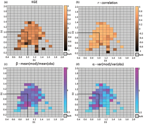
In Fig. 7(a) we can see how moving away from the centred and uniform position, the KGE score tends to show smaller values. Figure 7(b) does not seem particularly informative as most of the plot areas show a similar correlation value. Figure 7(c) shows how for localized events (D2 < 1 and in particular D2 < 0.5) the mean modelled value tends to generally be lower than the observed ones. This is expected as the model does not consider the spatial rainfall pattern of the event and therefore effectively distributes rainfall equally over the entire catchment area, resulting in higher infiltration. A stronger pattern is shown by Fig. 7(d), where the KGE variance of the modelled events is lower than that of the observed events for localized events, and in particular upstream. This also seems to reflect the expected behaviour, as the lumped model considers the rainfall to be uniform and therefore generates less peaked hydrographs which therefore show a low value of KGE variance.

Despite some grids of the D1–D2 plot (Fig. 7) showing unexpected results, which are further discussed in Section 5.3, the modelling investigation mostly confirms the expected behaviour. This strengthens the evidence for using moments of rainfall spatial variability not only to predict the differences in runoff response between spatially variable and uniform events, but also to help understanding when lumped rainfall information would affect the performance of hydrological forecasts and therefore a distributed rainfall information would be preferred. In this way practitioners will be guided to the most appropriate approach, rather than using the approach with which they are more experienced (Addor and Melsen 2019). Nevertheless, it is important to note that the modelling experiment here provides less strong links between rainfall spatial variability and the shape of the hydrograph compared to the direct comparison in Section 4.2. This demonstrates how the modelling approach, which involves multiple variables and processes, can contribute to the contradictory findings about the importance of rainfall spatial variability in shaping the hydrograph and how the novel approach can provide meaningful insight.

5 Discussion

As mentioned in Section 1, the importance of rainfall of spatial variability for runoff modelling is a debated topic (e.g. Obled et al. 1994 vs Cole and Moore 2008). The contradictory results and conclusions on the usefulness of the rainfall spatial pattern might be caused also by the small number of events for which this information matters. In our analysis the vast majority of the rainfall events occurring within the catchments analysed in Great Britain appear to be uniform, and hence the rainfall spatial pattern does not provide more information than catchment averages. However, especially when the majority of events show a uniform pattern, it is useful for practitioners to identify a priori events for which the rainfall pattern plays an important role in the runoff response. In this study we showed that moments of rainfall spatial variability are able to identify rainfall events that will generate longer/shorter or peaked/less peaked responses compared to uniform events happening in the same catchment. The novel approach allows researchers to confirm the appropriateness of moments for deciding between a lumped or a distributed rainfall information for operational hydrological modelling, reducing the number of a priori assumptions. The lumped hydrological analysis has shown how events that have been classified as spatially variable by moments are attributed to streamflow responses with lower performance scores than those attributed to uniform events. However, the link between moments values and model performance score is less clear than that between moments values and features of the observed hydrograph, indicating that there are certainly other sources of variability that play a role in shaping the runoff response and highlighting the importance of using the novel approach to reduce uncertainty in existing knowledge.

We discuss the above results along with any limitations in the following subsections.

5.1 Uniform rainfall events are much more frequent than spatially variable events

Rainfall events are spatially variable when rainfall itself is highly variable (e.g. thunderstorms) or when the extent of the storm is smaller than the catchment area (Zoccatelli et al. 2011, Lobligeois et al. 2014). Because in the UK the dominant mechanism for flood generation is excess rainfall (Stein et al. 2019) and thunderstorms are not as frequent as stratiform storms, we therefore mainly observe spatially variable rainfall events when the storm extent (during the time window equal to Tr of maximum rainfall) is smaller than the catchment area. However, in this work the study catchments areas are not very large, ranging from 16 to 1508 km², with a median value of 285 km². As the catchment areas are relatively small, it is more likely that the storm is fully covering the catchment extent compared to when catchment areas are larger. As a result, the rainfall spatial patterns will be mainly uniform and catchment centred. Moreover, the South East of England is where climatically we observe more short-duration intense rainfall events (Hand et al. 2004), but due to the criteria adopted for catchment selection, the study catchment set includes only three catchment in this area.

Another possible reason for the majority of events being uniform is the time scale at which moments were estimated. As the ultimate aim is to characterize the runoff peak, we computed the moments on the time window equal to Tr of maximum rainfall for each event. Certainly, if we calculated moments of rainfall spatial variability for the same events but on a shorter temporal scale than Tr (e.g. per hour), we would observe more variability and less uniform patterns. However, this would not necessarily be meaningful to describe the runoff peak. Nevertheless, in other studies we can see that different temporal scales have been taken into account for estimating moments of rainfall spatial variability (Zoccatelli et al. 2011; Lobligeois et al. 2014, Emmanuel et al. 2016), and the majority of events still appear uniform, especially when large numbers of events are examined (Lobligeois et al. 2014).

Another potential reason for such a frequent occurrence of uniform events could be related to the methodology used to build the CEH-GEAR1hr rainfall dataset. The interpolation of raingauge data may tend to smooth the rainfall field, consequently showing more uniform spatial patterns compared to the original gauge values (Cole and Moore 2009). The interpolation itself can impose a spatial correlation in the precipitation field which is strongly dependent on the number of raingauges within each catchment. However, we performed a similar analysis (see Supplementary material, Fig. S1) using a radar rainfall dataset provided by the UK Met Office ground-based weather radar network (Harrison et al. 2009) and the distribution of the spatial moments show a very similar pattern, meaning that the results are robust and do not depend on the rainfall dataset used.

In Figs 4 and 5, we also observe that the distribution of D1 and D2 values are slightly shifted towards upstream events. Hence, it seems that localized upstream events are slightly more frequent than localized downstream ones. The reason for this result might be that topography tends to enhance the cooling of water vapour, generating more precipitation in the headwaters (e.g. Hill et al. 1981, Hill 1983). In addition, we find that unimodal events are much more frequent than bimodal events (D2 < 1 more frequent than D2 > 1): this result could be related again to catchments’ size and temporal scale at which moments are estimated, but we suggest also that a bimodal distribution is quite a rare pattern because of the structure itself – two hotspots in the catchment but with their centroids at different distances from the catchment outlet. This distribution might also be more typical of thunderstorms, which are less frequent than stratiform events in the UK. Overall, it appears the majority of events could be simply treated using lumped rainfall information; hence, being able to identify a priori the events for which this would not be appropriate seems very useful for practitioners.

5.2 Moments of rainfall spatial variability show a relationship with timing and peakedness of the observed hydrograph

The first moment of rainfall spatial variability is able to identify when the position of the storm will produce slower or faster responses than centred events, while the second moment can indicate when the spatial variability will produce more peaked or flatter hydrographs than uniform events occurring in the same catchment. As expected, larger events show shorter response times (Dooge 1973) and higher runoff coefficients, but, interestingly, the effect of the rainfall spatial pattern is larger on smaller events than on larger events. This finding could help explain the contradictory results on the importance of spatial variability of rainfall for runoff response, as for different groups of events the rainfall spatial pattern appears more/less influential. The comparison between moments values and characteristics of the observed hydrograph generated by spatially variable events and by uniform events has confirmed the potential of the moments of rainfall spatial variability as a useful tool for operational hydrologists.

However, there are outliers (Fig. 6), meaning that, as we would expect, rainfall spatial variability is not the only factor influencing the shape of the hydrograph and spatial moments are not able to explain the entire hydrograph but just the response due to rainfall spatial variability. For example, moments of rainfall spatial variability can tell us when an event is localized downstream and hence will show a fast and sharply peaked hydrograph, but a similar response could also be caused by other factors (e.g. evapo-transpiration, soil moisture to full capacity, or a strong temporal pattern in the rainfall), causing some events to be represented in Fig. 6 as outliers.

In fact, among the factors playing a role there are certainly the antecedent conditions (e.g. soil moisture capacity, fast and slow component storage) but also spatial organization of other variables (e.g. potential evapotranspiration or soil moisture) and geology. According to the framework proposed by Woods and Sivapalan (1999) and revised by Viglione et al. (2010), and its extension by Mei et al. (2017) that includes faster and slower response components, there are many spatial and temporal interactions that we are neglecting in this study. However, for practical applications it is required to convert such complexity of interactions into simple tools which can be easily applied by practitioners to identify “unusual” behaviour. An attempt to integrate this complexity of interaction in a simple tool has been made in the context of flash flooding where a dynamic runoff coefficient (Raynaud et al. 2015), based on antecedent soil moisture conditions, has been developed to weight the rainfall-driven European Precipitation Index (Alfieri and Thielen 2015).

A simple way to start expanding our work to the multiple sources of variability would be to test the potential of moments of rainfall temporal variability on “real-world” events. Rainfall has been recognized for many years as having a primary role in shaping the hydrograph (Singh 1997, Winchell et al. 1998), hence its spatial pattern as much as its temporal one has a great impact on shaping the hydrograph. For example, Gaál et al. (2012) showed how the type of storm, which can be associated with a specific temporal rainfall distribution, can influence the flood duration. Developing simple tools such as the moments that enclose some of the variability of the processes affecting runoff response requires a number of assumptions. However, if the efficacy of these tools can be proven though a direct comparison with hydrograph characteristics, this could potentially be of substantial help to forecasters.

5.3 Rainfall events classified as spatially variable show a lower skill score when simulated by a lumped model

The information provided by moments of rainfall spatial variability can be considered meaningful as the performance of the lumped hydrological model for spatially variable events is generally lower than for uniform events (Fig. 7a). Although for larger events the impact of the rainfall spatial pattern seemed to be small (Fig. 6b), we can still observe the expected pattern in the lumped modelling performance (Fig. 7). In particular, when the rainfall is localized we can see how the KGE variance of the simulated event is underestimated compared to the observed one (Fig. 7d).

However, looking in detail at the different components, we observe for some of the localized events (D2 < 1) mean and variance of the model flow larger than the observed ones. If this seems counter-intuitive, we need to remember that the KGE and its components are evaluated on the entire event, while we computed the moments of rainfall spatial variability taking into account only the peak time. Especially for larger events, where we observed a less marked influence of the spatial pattern on runoff response (Fig. 6b), it is possible that other sources of variability not taken into account by the lumped hydrological model are playing a more important role.

Another reason for the lower or unexpected performance with a localized event could be related to the calibration process. In fact, in this study the models are calibrated using 50% of the whole record. As we saw in Section 4.1, the majority of the events show a uniform and centred spatial pattern, hence the models are trained mainly with this type of event. This could potentially affect the performance of the model when evaluated on spatially variable events, but a calibration for specific classes of events in each catchment would not be possible due to the small number of events falling in some groups. If using a distributed model would help in taking into account the rainfall spatial pattern, the problem of training a model on mainly uniform events would remain. In this context, the moments of rainfall spatial variability could be useful to identify when the simulation does not reflect the structure of the rainfall spatial pattern.

6 Conclusions

This work tests the usefulness of moments of rainfall spatial variability (Zoccatelli et al. 2011) for practical applications, using a direct comparison between moments values and characteristics of observed hydrographs generated by spatially variable events and by uniform ones in the same catchment. The reduced number of a priori assumptions used by the proposed approach allows us to confirm previous results with more confidence and to support the usefulness of moments in the choice between lumped and distributed rainfall information. Moreover, using a lumped model we further test the moments by checking whether the modelling performance of events classified as spatially variable is actually lower than that of uniform ones. Although uniform events make up the majority in the examined catchments in Great Britain, results show that the moments are able to identify the spatially variable events and tell us if their responses are going to be shorter/longer and more/less peaked than the uniform events in the same catchments, due to rainfall spatial pattern. The lumped modelling test has shown generally lower performance scores for spatially variable events compared to uniform ones. However, the pattern seems less clear than through the comparison with characteristics of the observed hydrograph, meaning that on the overall event simulation performance there are other sources of variability playing an equally important, or perhaps even more important, role and suggesting that the comparison with characteristics of the observed hydrograph actually provides useful insight for a better understanding of the role of spatial variability of rainfall.

The framework by Viglione et al. (2010) and its extension by Mei et al. (2017) highlight many other sources of variability playing a role in shaping the hydrograph. We believe that it would be useful to convert their mathematical formulations into simple tools by making some assumptions, as in Zoccatelli et al. (2011), and to test their usefulness for practical applications. As a result, practitioners could benefit more from the research studies and make use of this knowledge to identify unusual behaviour or check their hydrological forecasts. A first step in extending this work could be to consider the potential of moments of rainfall temporal variability and test them for practical applications. Moreover, further investigation will be required to assess whether the conclusions drawn in this study will still be valid for catchments affected by human impacts (including water management) and hence whether the information content of the moments could be used for flood forecasting in urbanized catchments.

Data availability

Information about the UK Benchmark Network can be obtained from the website https://nrfa.ceh.ac.uk/benchmark-network. Information about the digital elevation model can be obtained from the website http://catalogue.ceda.ac.uk/uuid/f5d41db1170f41819497d15dd8052ad2. Hourly streamflow time series are available on request from the Environmental Agency (EA), Natural Resources Wales (NWR) and Scottish Environmental Protection Agency (SEPA). CEH-GEAR1hr precipitation data are available from the website https://doi.org/10.5285/d4ddc781-25f3-423a-bba0-747cc82dc6fa. Information about the potential evapotranspiration (PET) dataset can be obtained from the website https://catalogue.ceh.ac.uk/documents/8baf805d-39ce-4dac-b224-c926ada353b7, and the code used to disaggregate daily to hourly PET estimates can be found at the website https://github.com/pamelaiskra/To_hourly/tree/master/PET.

Acknowledgements

Our thanks go to Gemma Coxon for help in data preparation.

Disclosure statement

No potential conflict of interest was reported by the authors.

Supplementary material

Supplemental data for this article can be accessed online at https://doi.org/10.1080/02626667.2022.2092405

Additional information

Funding

This work is funded as part of the Water Informatics Science and Engineering Centre for Doctoral Training (WISE CDT) under a grant from the Engineering and Physical Sciences Research Council (EPSRC) [grant number EP/L016214/1].

Appendix

In this appendix we present the equations used to analytically estimate the first moment (D1) and the second moment (D2) of rainfall spatial variability rainfall over a certain rainfall period T_s according to Zoccatelli et al. (2011). The code to compute the first and second moments is available at https://github.com/giuliagiani/Moments_spatial_variability_of_rainfall.

(A1) $D1=\frac{P_1}{P_0{g}_1},$(A1)

(A2) $D2=\frac{1}{g_2-g_1^2}\left[\frac{P_2}{P_0}-{\left(\frac{P_1}{P_0}\right)}^2\right],$(A2)

where

(A3) $P_n={\left|A\right|}^{-1}\underset{0}{\overset{A}{\int }}{r}_t\left(x,y\right)d{\left(x,y\right)}^{n}dA,$(A3)

(A4) $g_n={\left|A\right|}^{-1}\underset{0}{\overset{A}{\int }}d{\left(x,y\right)}^{n}dA,$(A4)

where A is the catchment area, $P_n$ is the nth integrated spatial moment of catchment rainfall over the time period T_s and $g_n$ the nth moment of flow distance. In the two equations $r_t(x,y$) is the mean value of time-integrated rainfall at location (x,y) and $d\left(x,y\right)$ is the distance between the position (x,y) and the catchment outlet measured along the flowpath.

For the calculation of the moments per time step the equations are the same, but we consider the value of rainfall at each individual time step at location (x,y), $r_t\left(x,y,t\right)$, instead of the mean value of time-integrated rainfall at location (x,y), $r_t(x,y$).

References

- Addor, N. and Melsen, L.A., 2019. Legacy, rather than adequacy, drives the selection of hydrological models. Water Resources Research, 55 (1), 378–390. doi:10.1029/2018WR022958
- Alfieri, L. and Thielen, J., 2015. A European precipitation index for extreme rain-storm and flash flood early warning. Meteorological Applications, 22 (1), 3–13. doi:10.1002/met.1328
- Asquith, W.H., et al. (2005). Summary of dimensionless Texas hyetographs and distribution of storm depth developed for Texas department of transportation research project 0-4914. Austin, Texas: U.S. Geological Survey. Report 0-4194-4.
- Bell, V.A. and Moore, R.J., 2000. The sensitivity of catchment runoff models to rainfall data at different spatial scales. Hydrology and Earth System Sciences, 4 (4), 653–667. doi:10.5194/hess-4-653-2000
- Beven, K.J., 2020. A history of the concept of time of concentration. Hydrology and Earth System Sciences, 24 (5), 2655–2670. doi:10.5194/hess-24-2655-2020
- Bonnifait, L., et al., 2009. Distributed hydrologic and hydraulic modelling with radar rainfall input: reconstruction of the 8–9 September 2002 catastrophic flood event in the Gard region (France). Advances in Water Resoures, 32 (7), 1077–1089. doi:10.1016/j.advwatres.2009.03.007
- Bracken, L.J., Cox, N.J., and Shannon, J., 2008. The relationship between rainfall inputs and flood generation in south-east Spain. Hydrological Processes, 22 (5), 683–696. doi:10.1002/hyp.6641
- Cole, S.J. and Moore, R.J., 2008. Hydrological modelling using raingauge- and radar-based estimators of areal rainfall. Journal of Hydrology, 358 (3–4), 159–181. doi:10.1016/j.jhydrol.2008.05.025
- Cole, S.J. and Moore, R.J., 2009. Distributed hydrological modelling using weather radar in gauged and ungauged basins. Advances in Water Resources, 32 (7), 1107–1120. doi:10.1016/j.advwatres.2009.01.006
- Das, T., et al., 2008. Comparison of conceptual model performance using different representations of spatial variability. Journal of Hydrology, 356 (1–2), 106–118. doi:10.1016/j.jhydrol.2008.04.008
- Dawson, C.W., Abrahart, R.J., and See, L.M., 2007. HydroTest: a web-based toolbox of evaluation metrics for the standardised assessment of hydrological forecasts. Environmental Modelling and Software, 22 (7), 1034–1052. doi:10.1016/j.envsoft.2006.06.008
- Dooge, J.C.I., 1973. Linear theory of hydrologic systems. Technical Bulletin 1468. US Department of Agriculture.
- Dunkerley, D., 2008. Identifying individual rain events from pluviograph records: a review with analysis of data from an Australian dryland site. Hydrolocigal Processes, 22, 5024–5036. doi:10.1002/hyp.7122
- Emmanuel, I., et al., 2016. Influence of the spatial variability of rainfall on hydrograph modelling at catchment outlet: a case study in the Cevennes region, France. FLOODRisk 2016, 3rd European conference on flood risk management, Oct 2016: LYON, France
- Emmanuel, I., et al., 2017. A method for assessing the influence of rainfall spatial variability on hydrograph modeling. First case study in the cevennes region, southern France. Journal of Hydrology, Elsevier, 555, 314–322. doi:10.1016/j.jhydrol.2017.10.011
- Euser, T., et al., 2015. The effect of forcing and landscape distribution on performance and consistency of model structures. Hydrological Processes, 29 (17), 3727–3743. doi:10.1002/hyp.10445
- Gaál, L., et al., 2012. Flood timescales: understanding the interplay of climate and catchment processes through comparative hydrology. Water Resources Research, 48 (4), W04511. doi:10.1029/2011WR011509
- Giani, G., Rico-Ramirez, M.A., and Woods, R.A., 2021. A practical, objective and robust technique to directly estimate catchment response time. Water Resources Research, 57 (2), e2020WR028201. doi:10.1029/2020WR028201
- Graeff, T., et al., 2012. Predicting event response in a nested catchment with generalized linear models and a distributed watershed model. Hydrological Processes, 26 (24), 3749–3769. doi:10.1002/hyp.8463
- Grimaldi, S., et al., 2012. Time of concentration: a paradox in modern hydrology. Hydrological Sciences Journal, 57 (2), 217–228. doi:10.1080/02626667.2011.644244
- Gupta, H.V., et al., 2009. Decomposition of the mean squared error and NSE performance criteria: implications for improving hydrological modelling. Journal of Hydrology, 377 (1–2), 80–91. doi:10.1016/j.jhydrol.2009.08.003
- Hall, M.J., 2001. How well does your model fit the data?. Journal of Hydroinformatics, 3 (1), 49–55. doi:10.2166/hydro.2001.0006
- Hand, W., Fox, N., and Collier, C., 2004. A study of the 20th-century extreme rainfall events in the United Kingdom with implications for forecasting. Meteorological Applications, 11 (1), 15–31. doi:10.1017/S1350482703001117
- Harrigan, S., et al., 2018. Designation and trend analysis of the updated UK Benchmark Network of river flow stations: the UKBN2 dataset. Hydrological Resources, 49 (2), 552–567.
- Harrison, D.L., Scovell, R.W., and Kitchen, M. (2009). High-resolution precipitation estimates for hydrological uses. Proceedings of the institution of civil engineers-water management, Vol. 162, No. 2, pp. 125–135, Thomas Telford Ltd.
- Hill, F.F., Browning, K.A., and Bader, M.J., 1981. Radar and raingauge observations of orographic rain over south Wales. Quarterly Journal of the Royal Meteorological Society, 107 (453), 643–670. doi:10.1002/qj.49710745312
- Hill, F.F., 1983. The use of average annual rainfall to derive estimates of orographic enhancement of frontal rain over England and Wales for different wind directions. Journal of Climatology, 3 (2), 113–129. doi:10.1002/joc.3370030202
- Intermap Technologies, 2009. NEXTMap British digital terrain 50m resolution (DTM10) model data by intermap. NERC Earth Observation Data Centre, 27 September 2020. http://catalogue.ceda.ac.uk/uuid/f5d41db1170f41819497d15dd8052ad2
- Knoben, W.J.M., Freer, J.E., and Woods, R.A., 2019. Technical note: inherent benchmark or not? Comparing Nash–Sutcliffe and Kling–Gupta efficiency scores. Hydrology and Earth System Sciences, 23 (10), 4323–4331. doi:10.5194/hess-23-4323-2019
- Kuichling, E., 1889. The relation between the rainfall and the discharge of sewers in populous districts. Transactions of the American Society of Civil Engineers, 20 (1), 1–56. doi:10.1061/TACEAT.0000694
- Kumar, M.R., Meenambal, T., and Kumar, V., 2019. Abstraction, ensemble, and disaggregation approaches to estimate evapotranspiration for use in hydrologic models. SIMULATION, 95, 116–199.
- Lewis, E., et al., 2019. Gridded estimates of hourly areal rainfall for Great Britain (1990-2014) [CEH-GEAR1hr]. NERC Environmental Information Data Centre.
- Lobligeois, F., et al., 2014. When does higher spatial resolution rainfall information improve streamflow simulation? An evaluation using 3620 flood events. Hydrology and Earth System Sciences, 18 (2), 575–594. doi:10.5194/hess-18-575-2014
- Mei, Y., Shen, X., and Anagnostou, E.N., 2017. A synthesis of space–time variability in multicomponent flood response. Hydrology and Earth System Sciences, 21 (5), 2277–2299. doi:10.5194/hess-21-2277-2017
- Monteith, J.L., 1965. Evaporation and the Environment. 19th symposia of the Society for Experimental Biology, 19, 205–234.
- Moore, R.J., 2007. The PDM rainfall-runoff model. Hydrology and Earth System Sciences, 11 (1), 483–499. doi:10.5194/hess-11-483-2007
- Norbiato, D., et al., 2009. Controls on event runoff coefficients in the eastern Italian Alps. Journal of Hydrology, 375 (3–4), 312–325. doi:10.1016/j.jhydrol.2009.06.044
- Obled, C., Wendling, J., and Beven, K., 1994. Sensitivity of hydrological models to spatial rainfall patterns: an evaluation using observed data. Journal of Hydrology, 159 (1–4), 305–333. doi:10.1016/0022-1694(94)90263-1
- Pilling, C., et al., 2016. Chapter 9- flood forecasting — a National overview for Great Britain. In: T.E. Adams and T.C. Pagano, eds. Flood forecasting. Academic Press, 201–247.
- Raynaud, D., et al., 2015. A dynamic runoff co-efficient to improve flash flood early warning in Europe: evaluation on the 2013 central European floods in Germany. Meteorological Applications, 22 (3), 410–418. doi:10.1002/met.1469
- Reed, S., et al., 2004. Overall distributed model intercomparison project results. Journal of Hydrology, 298 (1–4), 27–60. doi:10.1016/j.jhydrol.2004.03.031
- Robinson, E.L., et al., 2016. Climate hydrology and ecology research support system meteorological dataset (1961-2015). [CHESS-met] . NERC-Environmental Information Data Centre.
- Schwanghart, W. and Scherler, D., 2014. Short communication: topoToolbox 2 – MATLAB-based software for topographic analysis and modeling in earth surface sciences. Earth Surface Dynamics, 2 (1), 1–7. Copernicus GmbH. doi:10.5194/esurf-2-1-2014
- Sharpe, M. and Cranston, M., 2021. Extreme rainfall in Scotland on 11 and 12 August 2020: evaluation of impact-based rainfall forecasts. Weather, 76 (8), 254–260. doi:10.1002/wea.3981
- Singh, V.P., 1997. Effect of spatial and temporal variability in rainfall and watershed characteristics on stream flow hydrograph. Hydrological Processes, 11 (12), 1649–1669. doi:10.1002/(SICI)1099-1085(19971015)11:12<1649::AID-HYP495>3.0.CO;2-1
- Smith, M., et al., 2004. Runoff response to spatial variability in precipitation: an analysis of observed data. Journal of Hydrology, 298 (1–4), 267–286. doi:10.1016/j.jhydrol.2004.03.039
- Stein, L., Pianosi, F., and Woods, R., 2019. Event-based classification for global study of river flood generating processes. Hydrological Processes, 34 (7), 1514–1529. doi:10.1002/hyp.13678
- Viglione, A., et al., 2010. Generalised synthesis of space-time variability in flood response: an analytical framework. Journal of Hydrology, 394 (1–2), 198–212. doi:10.1016/j.jhydrol.2010.05.047
- Winchell, M., Gupta, V.H., and Sorooshian, S., 1998. On the simulation of infiltration and saturation excess runoff using radar-based rainfall estimates: effects of algorithm uncertainty and pixel aggregation. Water Resources Research, 34 (10), 2655–2670. doi:10.1029/98WR02009
- Woods, R. and Sivapalan, M., 1999. A synthesis of space-time variability in storm response: rainfall, runoff generation, and routing. Water Resources Research, 35 (8), 2469–2485. doi:10.1029/1999WR900014
- Zoccatelli, D. et al., 2011. Spatial moments of catchment rainfall: rainfall spatial organisation, basin morphology, and flood response. Hydrology and Earth System and Sciences, 15, 3767–3783. doi:10.5194/hess-15-3767-2011