Advancing traditional strategies for testing hydrological model fitness in a changing climate

ABSTRACT

Mitigation of adverse effects of global warming relies on accurate flow projections under climate change. These projections usually focus on changes in hydrological signatures, such as 100-year floods, which are estimated through statistical analyses of simulated flows under baseline and future conditions. However, models used for these simulations are traditionally calibrated to reproduce entire flow series, rather than statistics of hydrological signatures. Here, we consider this dichotomy by testing whether performance indicators (e.g. Nash-Sutcliffe coefficient) are informative about model ability to reproduce distributions and trends in the signatures. Results of streamflow simulations in 50 high-latitude catchments with the 3DNet-Catch model show that high model performances according to traditional indicators do not provide assurance that distributions or trends in hydrological signatures are well reproduced. We therefore suggest that performance in reproducing distributions and trends in hydrological signatures should be included in the process of model selection for climate change impact studies.

KEYWORDS:

• climate change
• hydrological signatures
• model evaluation
• runoff timing
• precipitation-runoff models
• trends

Editor S. Archfield Associate Editor R. Singh

1 Introduction

Global warming and changes in climate conditions can have adverse effects on water resources. They can affect water supply, irrigation or hydropower production (Xu 1999a), and, consequently, economy, safety and ecosystem sustainability (Olsson et al. 2016). In many regions around the world, global warming is expected to increase the frequency of hazardous events, such as floods (Dankers and Feyen 2009, Dankers et al. 2014) or droughts (Wasko et al. 2021), both of which cause substantial economic losses (Roudier et al. 2016). Global warming acts together with rapid urbanization and population growth in some regions, thereby increasing pressure on water resources and potentially leading to water scarcity (Schewe et al. 2014). Therefore, adequate strategic planning and implementation of optimal climate-change adaptation measures are of vital socio-economic importance (Gangrade et al. 2020), especially with regard to the realization of the Agenda 2030 Sustainable Development Goals that highlights the importance of water as an integral part of human development (United Nations Water 2015, WWAP (United Nations World Water Assessment Programme) 2015). However, the identification of relevant adaptation measures largely depends on reliable assessment of climate change impacts on water resources (Feng and Beighley 2020).

Climate change impacts on water resources are typically assessed by comparing simulated hydrological variables over a future period to those simulated in the baseline (i.e. historical/present) period (Hakala et al. 2019). Climate change impact studies (CCISs) are focused primarily on flows, since they represent an integrated catchment response to alterations in hydroclimatic processes (Beck et al. 2017). In particular, CCISs are concerned with changes in flow statistics (Olsson et al. 2016), such as mean, high or low flows (Lehner et al. 2006, Ludwig et al. 2009, Gosling et al. 2017, Mishra et al. 2020). Analyses of high flows (e.g. Booij 2005, Kay et al. 2009, Dams et al. 2015, Chen and Yu 2016) and low flows (e.g. Parajka et al. 2016, Pokhrel et al. 2021) are important because these types of events can have adverse and far-reaching consequences for societies and ecosystems (Pechlivanidis et al. 2016). Therefore, they are essential from the perspective of water resources management (Farmer et al. 2018). Changes in flow seasonality and timings, or duration of some specific flows, are also often analysed (Cayan et al. 2001, Stewart et al. 2005, Addor et al. 2014, Mendoza et al. 2016, Feng and Beighley 2020), since they can be significant from an economic and environmental point of view (Blöschl et al. 2017, Blöschl et al. 2019b, Wasko et al. 2020). These flow regime features (e.g. mean or extreme flows, runoff timings and durations) are hereafter referred to as hydrological signatures (McMillan 2021).

Future flows are obtained by running a hydrological model with the downscaled and bias-corrected outputs of a general circulation model (GCM), which is run assuming one or several greenhouse gas concentration trajectories, i.e. representative concentration pathways (Refsgaard et al. 2014, Hakala et al. 2019). The GCM outputs have rather coarse spatial resolution and have to be downscaled to be suitable for hydrological modelling (Xu 1999b, Refsgaard et al. 2014, Teutschbein et al. 2010). Distributions of the downscaled GCM outputs display strong biases compared to their observed counterparts (primarily precipitation and temperature); thus, they have to be bias-corrected before being used for hydrological simulations (Teutschbein and Seibert 2012, 2013). Bias-correction improves the accuracy in reproducing distributions of climatic variables, as well as the projected flows (Osuch et al. 2016, Hakala et al. 2019).

Projected changes in the hydrological signatures depend on the assumed trajectories, and on each element in the complex modelling chain (Velazquez et al. 2013); thus, they are accompanied by uncertainties (Prudhomme and Davies 2009a, 2009b). Extensive research on these uncertainties often indicates climate models as the key source of uncertainty in the projections (Wilby and Harris 2006, Minville et al. 2008, Bastola et al. 2011, Najafi et al. 2011, Teng et al. 2012, Karlsson et al. 2016, Joseph et al. 2018). However, in some cases uncertainties induced from hydrological models can be similar or even larger than uncertainties stemming from the climate models (Bosshard et al. 2013, Pechlivanidis et al. 2016, Eisner et al. 2017). For example, low-flow projections are highly sensitive to the choice of hydrological models, presumably due to their limited skills in reproducing low flows (Maurer et al. 2010; Velazquez et al. 2013, Vansteenkiste et al. 2014, Parajka et al. 2016, Gangrade et al. 2020, Huang et al. 2020).

Selection of a hydrological model is a key step in a modelling study (Beck et al. 2017, Addor and Melsen 2019), including CCISs (Lespinas et al. 2014, Seiller et al. 2017). However, identification of models that are suitable for CCISs is quite challenging, as modelling under changing climate has remained one of the unsolved problems in hydrology (Blöschl et al. 2019a). In particular, there is a lack of specific guidance on the evaluation of model suitability for CCISs, and on model selection (Fowler et al. 2018b). Model suitability for CCISs is often assumed to be equal to model transferability that implies consistently good performance across various climatic conditions encountered in the record period (Kirchner 2006, Krysanova et al. 2018, Motavita et al. 2019). Transferable models are generally deemed to reasonably represent runoff generation processes (Euser et al. 2013); thus, application of such models is expected to yield credible flow projections (Krysanova et al. 2018). Model transferability is traditionally appraised by applying a split- or a differential split-sample test (DSST) (Klemeš 1986). The latter is considered more indicative of model performance under contrasting climate conditions (Seibert 2003). Recently, several extensions of the DSST have been proposed to enable even more rigorous evaluation of model transferability (Coron et al. 2012, Thirel et al. 2015, Fowler et al. 2018b). However, despite its robustness, DSST can fail to identify transferable models in some instances (Fowler et al. 2018b). Furthermore, good performance under current conditions (Krysanova et al. 2018), proven by a DSST or an extension thereof (Fowler et al. 2018a) is no guarantee that the model can perform well under future climate. This can be attributed to potential modifications of catchment processes (Blöschl and Montanari 2010, Chiew et al. 2015) or even emergence of processes not encountered in the record period (Peel and Blöschl 2011).

Model performance is typically quantified in terms of numerical indicators (efficiency measures), such as Kling-Gupta (Gupta et al. 2009) or Nash-Sutcliffe (Nash and Sutcliffe 1970) coefficients. These performance indicators (hereafter referred to as indicators) are based on aggregated statistics of the residuals, i.e. differences between observed and simulated flow series (Yilmaz et al. 2010). As such, they cannot fully reveal all aspects of model performance (Crochemore et al. 2015). For example, these indicators are often skewed towards high flows (Legates and McCabe 1999). To put more emphasis on low flows, various flow transformations, such as logarithms, are applied (Oudin et al. 2006, Fenicia et al. 2007, Santos et al. 2018). Furthermore, numerous parameter sets can yield quite similar values of a performance indicator (equifinality, Beven and Binley 1992), even though they result in different simulated hydrographs, especially outside the calibration period (Wagener et al. 2003). In addition to these indicators, various hydrological signatures can be used to complement evaluations of model performance and facilitate model diagnostics (Yilmaz et al. 2008, Pfannerstill et al. 2014, Topalović et al. 2020, McMillan 2021), and can also be used as objective functions in the model calibration (Westerberg et al. 2011, Shafii and Tolson 2015). Evaluation of model performance in extreme flows, such as annual maxima (Mizukami et al. 2019), has been proposed in the literature. Studies on this topic show that high performance in extreme flows is difficult to achieve because model calibration generally leads to a “squeezing” of the flow distribution (i.e. distribution tails move towards the central value), leading to overestimation of low flows and underestimation of high flows (Farmer et al. 2018).

Notwithstanding the significant progress in the field of hydrological model evaluation, the gap between information offered by the standard evaluation procedures and traditionally used performance indicators, and the requirements of CCISs, still persists. This discrepancy can be attributed to different approaches to calibration and evaluation of hydrological and of climate models. The former models are conditioned to reproduce entire series, while the latter are expected (and limited) to reproduce distributions over a 30-year period (Ricard et al. 2019). Therefore, transferability of hydrological models cannot be fully translated into transferability in the impact-assessment domain (Chen et al. 2016). Fowler et al. (2018a) argued that research on model applicability under changing climate conditions is insufficient, and that there is still a clear need for novel, more robust model structures, innovative calibration strategies and modelling practices in general (Gelfan et al. 2020), including novel evaluation procedures that can identify the most suitable models for CCISs (Coron et al. 2012, Thirel et al. 2015).

Evaluation of hydrological model suitability for CCISs should be focused on hydrological signatures that are pertinent to these studies, such as extreme flows or signatures that have various eco-hydrological applications (Mendoza et al. 2015, Krysanova et al. 2017, 2018, Ricard et al. 2019). This is in line with the concept of model “fitness for the said purpose” (Xu 1999c). Evaluation of model suitability for CCISs should, thus, include distributions of the selected hydrological signatures, because the impact assessments rely on these distributions, rather than on the entire series. Model performance in reproducing distributions of signatures is seldom considered (e.g. Willems 2009), especially its potential links to commonly used performance indicators (Coffey et al. 2004). Nevertheless, the hydrological community recognized the importance of accurate reproduction of signatures’ distributions, so bias-correction of simulated flows was suggested to improve this aspect of model performance (González-Zeas et al. 2012, Farmer et al. 2018, Daraio 2020, Bum Kim et al. 2021). Alternatively, hydrological model parameters alone (Ricard et al. 2019), or together with parameters of a bias-correction transfer function, can be optimised to improve accuracy in reproducing signatures’ distributions in the baseline period (Ricard et al. 2020). Model ability to reproduce trends in the signatures should also be evaluated, since such trends can affect the assessment of impacts of future climate (Cunderlik and Ouarda 2009, Wasko et al. 2020). Accurate reproduction of the trends poses a challenge to hydrological modelling, and conflicting conclusions about model performance in this respect were reported (Lespinas et al. 2014, Fowler et al. 2020, Wasko et al. 2021).

In this paper, we hypothesized that commonly used performance indicators are not necessarily informative about hydrological model ability to reproduce observed (and potential future) distributions and trends in hydrological signatures relevant for climate change impact assessments. Such signatures include, for example, flow statistics (e.g. mean, maximum and minimum flows), or runoff timings and durations. To test this hypothesis, we (1) evaluated model performance in reproducing distributions and trends in series of the signatures, and (2) examined relationships between numerous performance indicators and model performance in terms of distributions and trends in the signatures. This study advances previous research on this subject by taking numerous indicators and signatures into consideration, and by comprehensively analysing relationships between these two facets of model performance. All analyses were conducted for 50 Swedish catchments, covering a wide range of hydroclimatic regimes in high latitudes.

2 Methodology

2.1 Catchments and data

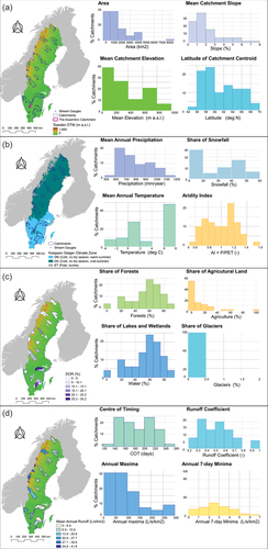
The study focuses on Sweden, a country in Northern Europe that covers an area of approximately 408 000 km² with an elevation range of −2 to 2100 m.a.s.l. (SLU 2015; Fig. 1(a)). The country’s area comprises 69% forests, 9% wetlands, 8% shrubs and grassland, 8% agriculture, 3% human settlements and 3% open land or glaciers. According to the Köppen-Geiger classification (Kottek et al. 2006), Sweden features three major climate zones: the polar tundra climate zone (ET) in the Scandinavian Mountains in northwestern Sweden, the subarctic boreal climate (Dfc) in central and northern Sweden, and the warm-summer hemiboreal climate zone (Dfb) in southern Sweden (Fig. 1(b)).

Figure 1. The selected catchments in Sweden and their properties: (a) locations of the catchments and distributions of their key topographic properties (area, slope, elevation and latitude); (b) climate of the selected catchments, and the distributions of mean annual precipitation, percentage of precipitation in the form of snowfall, mean annual temperature and the aridity index (ratio of mean precipitation to mean potential evapotranspiration); (c) degree of regulation (DOR, percentage of mean annual runoff from the drainage area of the reservoir) in the catchments and distributions of shares of prevailing land-use types, and water surfaces and glaciers; and (d) mean annual runoff in the catchments and distributions of the centre of timing (COT, in days of water year; Kromos et al. 2016), runoff coefficients, and annual maxima and seven-day minima. The hydroclimatic variables presented in the figure were obtained over water years 1962–2020.

Daily precipitation, temperature, and flow series for considered catchments over the period 1961–2020 were obtained from a publicly accessible database (http://vattenwebb.smhi.se/), maintained by the Swedish Meteorological and Hydrological Institute (SMHI). Geospatial data for the streamflow stations were downloaded from SMHI’s Svenskt Vattenarkiv (SVAR) database (Eklund 2011, Henestål et al. 2012). Daily temperature and precipitation series were obtained from the SMHI’s spatially interpolated 4 km × 4 km national precipitation–temperature grid (Johansson 2000, SMHI 2005). Mean catchment precipitation and temperature were calculated as an area-weighted average of all grid cells partly or fully lying within the catchment boundaries.

Only catchments for which continuous daily series from January 1961 to December 2020 were available, and which had low percentages of lakes, glaciers and urbanized areas and a low degree of regulation (DOR, i.e. reservoir volume relative to the mean annual runoff volume from its draining area; Fig. 1(c)) were selected for this study. Regarding the DOR criterion, the catchments were selected according to the results of preliminary analyses, rather than according to a specific threshold. Specifically, we selected only those catchments (1) for which inspection of hydrographs failed to detect any abrupt changes, and (2) for which modelling results, including those presented in the relevant literature on Swedish catchments (Girons Lopez et al. 2021), showed satisfactory model performance. Such catchments were considered not heavily regulated, and, therefore, suitable for this study. Only 50 catchments met all the criteria above, six of which were nested within larger catchments. Seventeen selected catchments were regulated (principally with DOR below 15%; Fig. 1(c)), with the dams that were built before 1961. Key properties of the selected catchments are presented in Fig. 1 and in Table S1 of the Supplementary material.

The 50 high-latitude catchments in this study span a latitudinal gradient from 56°N to 68°N and thus adequately reflect spatial variations in Swedish climate, topography, and land use (Fig. 1(b), Table S1). Over the past 60 years (1961–2020), annual mean temperature in those catchments was on average 2.7°C, with an annual precipitation of 762 mm. In half of the catchments, snowfall comprised approximately one third of annual precipitation, which is consistent with the relatively low mean annual temperatures, which were below 0°C in some catchments (Fig. 1(b)). The selected catchments were mainly snow-dominated (20 catchments) or transitional (21 catchments), while only nine catchments were rain-dominated according to the centre of timing (Kormos et al. 2016; Fig. 1(d)). Aridity indices, which were mainly lower than 1.5, suggest that the selected catchments are predominantly humid (UNEP 1992, Wang et al. 2021). Median annual runoff in the selected catchments was 379 mm (12 L/s/km²) over the record period. However, there were considerable spatial variations: specifically, the highest runoff was observed in the Scandinavian Mountains in northwestern Sweden, characterized by mountain snowmelt, and the lowest in southeastern Sweden (Fig. 1(d)), featured by less pronounced flow peaks. Hydrological regimes of the selected catchments are characterized by relatively high runoff coefficients (greater than 0.5) and high baseflow rates, i.e. baseflow index exceeded 0.5 in most catchments. Mean annual runoff was positively skewed in most catchments, suggesting a tendency towards occurrences of high flows (Carlisle et al. 2017).

2.2 The 3DNet-Catch model

In this study, runoff was simulated with the 3DNet-Catch model (Todorović et al. 2019). This model requires precipitation, temperature, and potential evapotranspiration series for simulations, and observed flows for calibration. Hydrological simulations consist of runoff simulations and routing, and can allow for correction of precipitation and temperature with elevation in semi- or fully-distributed set-ups (Stanić et al. 2018, Todorović et al. 2019).

2.2.1 Model structure

Runoff is simulated by employing the interception, snow and soil routines (see Figure S1 of the Supplementary material). Interception is modelled by a single storage with a flexible capacity that varies according to the leaf area index. All precipitation that occurs at temperatures below a particular threshold is considered snow. Snowmelt is simulated by applying the degree-day method with a seasonally varying melt factor. Spatial heterogeneity of the snow cover and snowpack sublimation are also accounted for. In the 3DNet-Catch model, soil is represented by a surface layer and an arbitrary number of subsurface layers that can have different parameters, such as thickness or porosity. Surface runoff, percolation, and evaporation take place in the surface layer (Todorović et al. 2019). Surface runoff is simulated by applying the Soil Conservation Service Curve Number (SCS-CN) method (Mishra and Singh 2003), which is combined with continuous simulation of soil moisture. Surface runoff can be augmented by the excess water from subsurface soil layer(s). Percolation into the deeper soil layer is simulated by using an analytically solved non-linear outflow equation combined with the Brooks-Corey relation (Brooks and Corey 1964). The water balance of the subsurface layer(s) comprises percolation from above as the inflow, and percolation to a deeper layer, or non-linear reservoir, and transpiration as outflows. Both linear and non-linear outflow equations are employed for runoff routing to a catchment outlet. Surface runoff is simulated with a linear outflow equation. Percolation from the deepest soil layer represents inflow to the non-linear reservoir with a threshold: water that exceeds the threshold is routed by an additional linear reservoir and produces subsurface runoff. Water below the threshold is routed by employing the non-linear equation and produces baseflow.

The chosen 50 catchments were characterized by relatively low variations in land use and in elevation span; hence, a spatially lumped model set-up was used in this study, without any corrections of meteorological variables with elevation. The adopted model version has one surface and one subsurface soil layer that share the same parameters, except for thickness and hydraulic conductivity. This model version has 21 free model parameters (see Table S2 of the Supplementary material for parameter list and their prior ranges).

2.2.2 Model calibration and evaluation

For each of the 50 catchments, model parameters were estimated in the first half of the record period (water years 1962–1991), and evaluated in the remainder (water years 1991–2020). Additionally, the model was run in the full record period (water years 1962–2020). All simulations were conducted at a daily time step, with one preceding water year for model warm-up. The model parameters were estimated by applying the Generalised Likelihood Uncertainty Estimation (GLUE) method (Beven and Binley 1992). For each catchment, only one best-performing set was chosen out of an initially sampled population of 75 000 from the uniform parameter prior distributions generated with the Latin hypercube sampling (Keramat and Kielbasa 1997). The parameter prior distributions were common to all catchments (Table S2). The best set in each catchment was selected according to a composite objective function (OF) that includes Kling-Gupta efficiency (KGE; Gupta et al. 2009) computed from daily flows and inverse-square root transformed flows (see Table 2 for equations) as follows:

(1) $OF=0.8KGE+0.2KG{E}_{1/\sqrt{Q}}$(1)

This composite OF was selected to obtain balanced performance in high and low flows (Santos et al. 2018, Mizukami et al. 2019). Although no optimization algorithm was employed in this study, the term “objective function” is nevertheless used to distinguish it from other performance indicators used for the analyses.

To examine impacts of parameter equifinality, we analysed the performance of the 50 best behavioural parameter sets in one catchment. The best sets were selected from the 75,000 initially sampled ones, based on their values of OF (Equation 1(1) $OF=0.8KGE+0.2KG{E}_{1/\sqrt{Q}}$(1) ) in the calibration period. As the reference catchment we selected Assembro (Fig. 1(a)), since it is a lowland, medium-sized catchment in central-south Sweden with catchment characteristics that correspond relatively well to the average characteristics of the selected catchment set, primarily in terms of hydrological regime features. Specifically, this is a transitional catchment (according to criteria by Kormos et al. 2016), with a runoff coefficient of 0.5 and a negligible percentage of lakes (7.4%). The number of behavioural sets was set to 50 to make the results of this simulation comparable to those conducted in the 50 catchments. The objective of the analyses with the best behavioural sets was to examine whether equifinality in terms of performance indicator(s) translates into equifinality in performance in reproducing distributions or trends in the series of signatures. Posterior parameter distributions (with OF as a likelihood measure), or ensembles of simulated flows with the behavioural sets, were not considered as testing the hypothesis of this study did not necessitate such results.

2.3 Evaluation of model performance in reproducing statistical properties of hydrological signatures

2.3.1 Selection of hydrological signatures

To assess the ability of 3DNet-Catch to reproduce hydrological signatures relevant for CCISs, we compiled a suite of signatures (Table 1). In addition to mean flows (Q_mean), the spring flows were analysed (Q_spring, March through June) to detect changes in runoff seasonality, which can be anticipated in high-latitude catchments in a warmer future climate due to a decrease in snowpack and its duration, and earlier snowmelt (Harder et al. 2015, Teutschbein et al. 2018, Kiesel et al. 2020).

Extremely high and low flows of given durations (e.g. annual daily maxima or minimum seven-day flows) are often used for assessment of flood hazard and environmental flows, and are important for consideration of climate change impacts on ecological and social systems (Gain et al. 2013). Assessment of climate change impacts on design floods is essential for dam safety (Bergström et al. 2001); therefore, the hydrological model should accurately reproduce distributions of maximum flows. Annual minima of given duration, or number of days with flows below a certain threshold, are relevant for assessment of allowable water withdrawals, including water supply withdrawals, or for the assessment of allowable loads from treatment plants, all of which are important for competent water management (Richter et al. 1996, Vis et al. 2015). As there are considerable uncertainties in simulating such extreme flows (Mizukami et al. 2019), the analyses in this study were complemented by moderately low and moderately high flows, represented by different flow percentiles (Gudmundsson et al. 2012).

Impact studies are often focused on changes in flow durations and timings that represent runoff seasonality (McMillan 2021). Consequently, model performance in reproducing runoff timing should be preferred over model efficiency in pre-defined subperiods (seasons), since these periods can vary over the years, especially under changing climate. Runoff timings are commonly computed from ordinal day of a calendar year and converted to a corresponding angular value between 0 and 2π (Cayan et al. 2001). Alternatively, runoff timings can be linearized if computed according to water years starting on 1 October (Wasko et al. 2020), which is the approach adopted in this study. Details on the selected hydrological signatures are presented in Table 1.

2.3.2 Evaluation of model performance in reproducing distributions of the hydrological signatures

In some studies, model performance in extreme flows was conducted by comparing some specific flow quantiles obtained from observed and simulated flows, such as 100-year floods (Dankers et al. 2014, Hoang et al. 2016). However, fitting a distribution, which includes selection of a distribution function and parameter estimation method, significantly affects estimated quantiles, particularly for high return periods, and can, therefore, affect reasoning on model performance in reproducing distributions of signatures (Dankers and Feyen 2009). Therefore, such an approach was not adopted here, and model evaluation was limited to a comparison of the series signatures obtained from observed and simulated flows.

Model ability to reproduce distributions of the selected signatures was conducted in (1) various catchments with different hydrological regimes, and (2) different periods. This set-up was adopted to reveal whether potential relationships between performance indicators and model ability to reproduce the distributions remain consistent across hydrological regimes and periods (Potter et al. 2010, Hannaford et al. 2013). Additionally, the analyses were repeated with numerous behavioural parameter sets (Beven and Binley 1992) in one catchment to examine whether equifinality in terms of performance indicators also implies equifinality in reproducing distributions of signatures.

The Wilcoxon rank sum (WRS) test (Conover 1999) was employed to evaluate model ability to reproduce distributions of the observed hydrological signatures. WRS is a nonparametric test used to compare continuous distributions of two samples, which do not necessarily have to be of the same size (Asadzadeh et al. 2014). The test does not imply any assumptions on the true form of probability distributions of the analysed variables, i.e. the two samples do not have to be normally distributed or equal in size (Kottegoda and Rosso 2008), and they can contain ties (García-Portugués 2022). The null hypothesis (H0) of the WRS test is that the medians of the samples’ distributions are equal, with the underlying assumption that the two distributions have the same shape and variance (Montgomery and Runger 2003). The WRS test statistic, z, is considered normally distributed if the sample size is greater than 15 (Kottegoda and Rosso 2008).

To evaluate model ability to reproduce distributions, annual series of the selected hydrological signatures (Table 1) were obtained from daily observed and simulated flows. These series were compared by applying the WRS test: in the case that the test null hypothesis was not rejected at a 5% level of significance, we assumed that the model reproduced distribution of a signature to a satisfactory degree.

2.3.3 Evaluation of model performance in reproducing trends in hydrological signatures

Model performance in reproducing trends has become an important part of model evaluation, particularly in the context of CCISs (Lespinas et al. 2014, Pechlivanidis et al. 2016, Hattermann et al. 2017). However, a common, systematic approach to evaluating this aspect of model performance has not been adopted yet. In this paper, a model was considered to properly reproduce a trend in a series if either (1) trends in the series obtained from both observed and simulated flows were not statistically significant, or (2) trends in both series were statistically significant and had the same sign. Otherwise, we considered that the model did not properly reproduce trends.

The Mann-Kendall test (Kendall 1938, Mann 1945) with a 5% of level of significance was applied to identify statistically significant trends in the hydrological signatures. The test was run in all 50 catchments (again for the calibration, evaluation and full record periods), as well as for the model runs with the 50 best parameter sets in the Assembro catchment over the calibration period. Serial autocorrelation can affect the results of this test (e.g. Fatichi et al. 2009, Harder et al. 2015) and, therefore, all considered series were tested for the presence of autocorrelation by applying the Box-Ljung test (Ljung and Box 1978) prior to testing for the presence of a trend. Thereafter, the Sen’s slope estimator was used to determine the sign of a trend (Sen 1968).

2.4 Relationships between performance indicators and hydrological signatures

2.4.1 Selection of performance indicators

Numerous performance indicators can be used to quantify model efficiency (Crochemore et al. 2015), and an entire set of indicators can be attributed to every simulated flow series. In the present study, 18 indicators were chosen to represent model performance (Table 2), including indicators focused on performance in high flows (e.g. KGE or Nash-Sutcliffe (NSE) coefficients), low flows (KGE or NSE computed from transformed flows or low-flow segments of flow duration curves), runoff volume (VE) or dynamics (coefficient of determination R²). Indicators based on the squared residuals, such as NSE, and on absolute values of residuals, such as index of agreement (IA), were included (Willmott et al. 2012), as well as indicators computed from flow duration curve segments (Pfannerstill et al. 2014, Todorović et al. 2019). All selected indicators are dimensionless, with higher values suggesting better model performance. A vValue of 1 indicates perfect fit according to all selected indicators, and almost none of the indicators has a lower limit (except for R², which takes values between 0 and 1).

Selection of the indicators was conditioned by the set-up of analyses of their informativeness about model ability to reproduce statistical properties of signatures. Specifically, some analyses within this study necessitated a monotonic relationship between the value of the performance indicator and model efficiency, and could not be conducted with e.g. percent bias in runoff volume, which can take positive and negative values, and where a value of 0 indicates a perfect fit. The selected performance indicators were calculated separately for each of the 50 catchments for the calibration, evaluation and full record periods, as well as for the 50 best model runs in the Assembro catchment in the calibration period (GLUE).

2.4.2 Informativeness of performance indicators about model performance in reproducing distributions of hydrological signatures

To analyse whether a specific performance indicator can provide insights about the model ability to reproduce distributions of hydrological signatures, we divided the simulations in the 50 catchments (separately for the calibration, evaluation and full record periods), as well as the simulations conducted with the 50 best parameter sets in Assembro, into two groups. One group comprised simulations that properly reproduced distributions according to the WRS test, and the second group included simulations that did not (i.e. H0 of the WRS test was rejected at a 5% level of significance). The values of a performance indicator of the two groups were then compared by applying another WRS test (for the sake of clarity, this particular test is denoted the WRS-2 test hereafter). Rejection of H0 at a 5% level of significance suggests that the median values of the performance indicators of the two groups were different. The alternative hypothesis of the WRS-2 test stated that the median of the indicators of the first group of simulations was greater than the median of the second group. As larger indicator values suggest better model performance, a rejection of the null hypothesis in favour of this alternative hypothesis suggests that higher indicator values would be indicative of better model performance in reproducing distributions of the selected signature. In other words, rejection of H0 of the WRS-2 test would suggest that a particular indicator can be informative about model ability to reproduce the distributions.

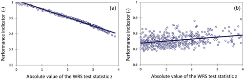
Further examinations of the relationships between performance indicators and model performance in reproducing distributions were based on Pearson correlation coefficients between values of indicators and absolute values of the WRS test statistic, z. High absolute values of the WRS test statistic suggest that it is within the rejection region and, thus, that the distributions are not well reproduced. For example, test statistics greater than 1.96 (or smaller than −1.96) imply rejection of H0 at the 5% level of significance (Kottegoda and Rosso 2008). Since this is a two-tailed test, absolute values of the test statistic are analysed. Strong negative correlations between the values of indicators and the absolute z values would suggest that higher indicator values would be informative about model ability to simulate the distributions of signatures (Fig. 2(a)). Here, correlation coefficients below −0.7 were considered an indication of strong correlation (Blasone et al. 2007). Weak negative or positive correlations would suggest that the indicators are not informative about model performance regarding distributions of signatures (Fig. 2(b)).

Figure 2. Illustration of relationships between performance indicator values and the absolute values of the Wilcoxon rank sum (WRS) test statistic. Larger values of performance indicators imply higher model efficiency, while larger absolute values of the test statistics imply rejection of the WRS test null hypothesis, i.e. the signatures obtained from the observed and simulated flows have statistically different medians. Panel (a) illustrates a performance indicator that can be considered informative about model ability to simulate the distribution of a signature, while panel (b) illustrates a non-informative indicator.

2.4.3 Informativeness of performance indicators about model performance in reproducing trends in hydrological signatures

To examine whether a specific indicator was informative in terms of model ability to reproduce trends, we followed the same logic as for the analysis of the distributions. The set of simulations was divided into two groups: one group containing the simulations that were able to reproduce trends according to the set criteria and one group containing all other simulations. The indicator values of the two groups were again compared using the WRS-2 test. Rejection of the WRS-2 test null hypothesis at a 5% level of significance in favour of the alternative hypothesis would suggest that higher indicator values could be used as an indication of model ability to reproduce trends in a simulation period.

3 Results

3.1 Hydrological model: overall performance of 3DNet-Catch

For each catchment, one parameter set that yielded maximum values of the composite OF (Equation 1(1) $OF=0.8KGE+0.2KG{E}_{1/\sqrt{Q}}$(1) ), which included KGE values computed from daily flows and reciprocals of square root-transformed flows (KGE_1/√Q), was selected. The median values of the OF across the catchments varied between 0.71 (evaluation) and 0.76 (calibration). The minimum values of the OF ranged between 0.41 (evaluation) and 0.73 (GLUE), while the maximum values ranged between 0.75 (GLUE) and 0.88 (calibration). No clear relationship between the values of the OF and the geographical location of the catchments was found (Fig. 3). For example, slightly lower values of the OF were obtained in a few catchments in the northwest of Sweden at high elevations, but also in a few catchments in mid and southern Sweden. The highest values of the OF were obtained in a few catchments in the northeast and southwest of the country. Performance in the smaller, nested catchments was quite similar to performance in the larger catchments encompassing them (Table S3 of the Supplementary material). Ranges of the OF values were rather consistent across the three simulation periods, while low variation across the GLUE behavioural sets suggests strong equifinality.

Figure 3. Model performance across the 50 catchments in the calibration (left), evaluation (mid) and full record periods (right panels). Model performance is quantified in terms of the objective function (OF, Equation 1(1) $OF=0.8KGE+0.2KG{E}_{1/\sqrt{Q}}$(1) ; panels a–c), and Kling-Gupta efficiency coefficients obtained from daily flows (KGE; panels d–f) and log-transformed flows (KGE[1/√Q]; panels g–i).

The median values of the majority of the performance indicators were satisfactory (Fig. 4), including KGE and KGE_1/√Q, generally suggesting a fair balance between the two parts of the OF. The highest median values (>0.9) were obtained for the IA across the simulations. Good performance was also achieved in terms of VE, showing that the model can accurately simulate runoff volume. The median VE values ranged from 0.92 in the full record period to 0.95 in the GLUE simulations. Another indicator with quite high values was KGE_fdc (the median values ranged between 0.88 and 0.92), suggesting that the model, on average, accurately reproduced the flow duration curve (FDC) in all simulation periods. The poorest performance, on average, was obtained in reproducing the lowest-flow FDC segment (KGE_95–100), especially in the GLUE simulations that yielded negative medians of this indicator. The median values of all the other indicators exceeded 0.50; however, there were some variations across the simulations: the highest median performance was obtained in the calibration period, while performance in the remaining simulations was slightly lower in most indicators. A few exceptions in this regard included KGE computed over two low-flow segments (namely, KGE_95–100 and KGE_70–100), which yielded very slightly higher values in the evaluation period.

Figure 4. Model performance in the 50 catchments in the calibration, evaluation and full record periods, and performance of the 50 best parameter sets in the Assembro catchment in the calibration period. Boxes indicate 25^th, 50^th and 75^th percentiles, while the whiskers stretch to the point nearest to 1.5 times the interquartile range from the boxes. Outliers and negative values are omitted from the figures for clarity. Abbreviations for the performance indicators are explained in Table 2.

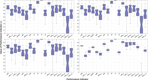
Table 1. Hydrological signatures (flow statistics, and runoff timings and durations) used for model evaluation.

Hydrological signature	Description	Reference
Mean annual flow, Qmean	Mean flows in a water year.
Mean spring flow, Qspring	Series of mean flows in the spring (1 March through 31 May) over the simulation period.	(Chen et al. 2017)
1-, 5- and 30-day maximum annual flows, Qmax,d for d = 1, 5 and 30	Series of annual maxima obtained from daily flows averaged over 5 and 30 days in each water year of the simulation period.	(Dankers et al. 2014, Vis et al. 2015)
1-,3-, 7-, 10-, 20-, 30- and 90 day minimum flows, Qmin,d for d = 1, 3, 7, 10, 20 and 30	Series of minimum flows averaged over a given number of days (d) obtained in each water year of the simulation period.	(Richter et al. 1996, Olden and Poff 2003, Garcia et al. 2017)
10^th and 90^th flow percentiles in wet seasons, Qwet,10p and Qwet,90p	Series of specific flow percentiles obtained in each water year of the simulation period. The wet season is defined as the period from 1 April through 30 September.	(Yarnell et al. 2020)
10^th and 90^th flow percentiles in dry seasons, Qdry,10p and Qdry,90p	Series of specific flow percentiles obtained in each water year of the simulation period. The dry season is defined as the period from 1 October through 31 March.	(Yarnell et al. 2020)
Timing of the centre of mass of annual flow, COM	Timing is computed from daily flows Qi and for each year in a simulation period:$COM=\sum i{Q}_i{t}_i\sum i{Q}_i$where ti represents the ordinal day of a water year.	(Mendoza et al. 2015, Kormos et al. 2016)
Spring onset (spring “pulse day”), SPD	Spring onset is the ordinal number of the day in which the negative difference between the streamflow mass curve and the mean streamflow mass curve is the greatest. Spring onset series is obtained from values in each water year of a simulation period.	(Cunderlik and Ouarda 2009)
High-flow frequency, HFF	Series of mean number of days in a water year with flows greater than 5 times the mean observed flow in the simulation period. In the literature, flows greater than nine times the mean observed flow are used for high-flow frequency computations. Since the catchments considered in this paper exhibited relatively low flow variability, this threshold was reduced to 5.	(Westerberg and McMillan 2015, Krysanova et al. 2017)
Low-flow frequency, LFF	Series of mean number of days in a water year with flows smaller than 20% of the mean observed flow in the simulation period.	(Nicolle et al. 2014, Westerberg and McMillan 2015, Krysanova et al. 2017)
Timing of the maximum annual flow, TQmax	Ordinal days in which maximum annual flow occurred, obtained in each water year of the simulation period.	(Richter et al. 1996)
Timing of the minimum annual flow, TQmin	Ordinal days in which minimum annual flow occurred, obtained in each water year of the simulation period. If there are several consecutive days with the same minimum flows, the mean timing of these days in a water year is adopted.	(Vis et al. 2015, Parajka et al. 2016)

Table 2. Performance indicators used for model evaluation.

Notation	Description of performance indicator and references	Equation
KGE	Kling-Gupta efficiency coefficient is computed from: daily flows, KGE (Gupta et al. 2009); reciprocal of root-transformed daily flows, KGE1/√Q, to put more emphasis on low flows (Santos et al. 2018); daily flows in a representative year, KGEwy, obtained by averaging daily flows on a specific calendar day over the entire simulation period (Schaefli et al. 2014)	$KGE=1-\sqrt{{\left(r-1\right)}^2+{\left(\alpha -1\right)}^2+{\left(\beta -1\right)}^2}$$r=\sum Ni=1\left(Q_{obs,i}-{\overline{Q}}_{obs}\right)\left(Q_{sim,i}-{\overline{Q}}_{sim}\right)\sum Ni=1{\left(Q_{obs,i}-{\overline{Q}}_{obs}\right)}^2{\left(Q_{sim,i}-{\overline{Q}}_{sim}\right)}^2$$\alpha =\frac{{\hat{S}}_{Q_{sim}}}{{\hat{S}}_{Q_{obs}}},\beta =\frac{{\bar{Q}}_{sim}}{{\bar{Q}}_{obs}}$
NPKGE	Non-parametric formulation of KGE indicator (Pool et al. 2018). It is computed as KGE, with Spearman instead of Pearson correlation coefficient, and with the ratio of standard deviations estimated from FDCs.	$NPKGE=1-\sqrt{{\left(r_{Spearman}-1\right)}^2+{\left({\alpha }_{NP}-1\right)}^2+{\left(\beta -1\right)}^2}$${\alpha }_{NP}=1-\frac{1}{2}\sum Ni=1\left|\frac{FD{C}_{sim,i}}{N{\overline{Q}}_{sim}}-\frac{FD{C}_{obs,i}}{N{\overline{Q}}_{obs}}\right|$
NSE	Nash-Sutcliffe efficiency coefficients (Nash and Sutcliffe 1970) are computed from daily (NSE) and log-transformed daily flows (NSElogQ).	$NSE=\sum Ni=1{\left(Q_{obs,i}-Q_{sim,i}\right)}^2\sum Ni=1{\left(Q_{obs,i}-{\overline{Q}}_{obs}\right)}^2$
LME	Liu mean efficiency represents a modification of KGE computed from daily flows (Liu 2020).	$LME=1-\sqrt{\left[{\left(k_1-1\right)}^2+{\left(\beta -1\right)}^2\right]}$$k_1=r\frac{{\hat{S}}_{Q_{sim}}}{{\hat{S}}_{Q_{obs}}}=\alpha r$
R^2	Coefficient of determination (Krause et al. 2005).	$\sum Ni=1\left(Q_{obs,i}-{\overline{Q}}_{obs}\right)\left(Q_{sim,i}-{\overline{Q}}_{sim}\right)\sum Ni=1{\left(Q_{obs,i}-{\overline{Q}}_{obs}\right)}^2\sum Ni=1{\left(Q_{sim,i}-{\overline{Q}}_{sim}\right)}^2$
VE	Volumetric efficiency (Criss and Winston 2008).	$VE=1-\sum Ni=1\left|Q_{sim,i}-Q_{obs,i}\right|\sum Ni=1Q_{obs,i}$
IA	Index of agreement (Krause et al. 2005).	$IA=1-\sum Ni=1{\left(Q_{obs,i}-Q_{sim,i}\right)}^2\sum Ni=1{\left(\left|Q_{obs,i}-{\overline{Q}}_{obs}\right|-\left|Q_{sim,i}-{\overline{Q}}_{obs}\right|\right)}^2$
LE	Lindström efficiency coefficient (Seibert and Vis 2010).	$LE=NSE-0.1\sum Ni=1\left|Q_{obs,i}-Q_{sim,i}\right|\sum Ni=1Q_{obs,i}$
KGEFDC	KGE computed from: entire flow duration curve (KGEFDC) (e.g.Todorović et al. 2019); and different flow duration curve (FDC) segments. The FDC segments are set after recommendations by Pfannerstill et al. (2014). Segments are obtained from flows that are exceeded given the percentage of time of the simulation period.	FDC segments considered: extremely high flows exceeded up to 5% of the time (KGE0–5), high flows: exceeded 5–20% of the time (KGE5–20), mean flows, exceeded 20–70% of the time (KGE20–70), low flows, exceeded 70–95% of the time (KGE70–95), very low flows, exceeded 95–100% of the time (KGE95–100), overall low flows, exceeded 70–100% of the time (KGE70–100).

* Q_obs – observed daily flows; Q_sim – simulated daily flows; ${\bar{Q}}_{\mathrm{o}\mathrm{b}\mathrm{s}}$ – mean observed flow over the simulation period; ${\bar{Q}}_{sim}$ – mean simulated flow over the simulation period; N – length of a simulation period (in days); ŝ – standard deviation; FDC – flow duration curve.

The values of high percentiles of the indicators in Fig. 4 showed that good performance could be obtained for all the indicators, with exception of KGE_95–100 in the GLUE simulations. High percentiles of Nash-Sutcliffe coefficients (NSE, NSE_logQ) and KGE computed from the transformed flows (also shown in panels g–i of Fig. 3) were slightly lower in comparison to the other indicators. In contrast, the low percentiles of the indicators showed that the model in some catchments or with some behavioural parameter sets yielded poor performance on many indicators, especially those related to the extreme flows (KGE computed over the highest and lowest FDC segments, KGE_0–5, KGE_95–100). An exception in this regard is IA, which consistently took rather high values. It should be emphasized that a high spread between low and high percentiles of the indicators was desired in this study in order to enable analyses of relationships between the indicators and model performance in reproducing distributions or trends in signatures. On the other hand, low variations across the indicator values of the GLUE sets were essential to enable proper analyses of equifinality impacts on model performance in reproducing distributions or trends in the series of signatures.

3.2 Model performance in reproducing statistical properties of hydrological signatures

3.2.1 Model performance in reproducing distributions of the hydrological signatures

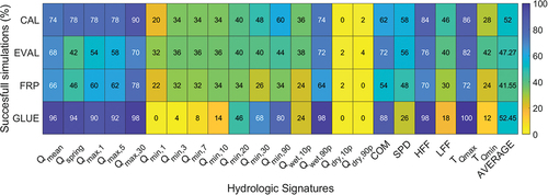
Distributions of the hydrological signatures were, on average, well reproduced by the model in most catchments (Fig. 5). High performances were obtained in mean flows (Q_mean), and for most signatures related to high flows (30-day annual maxima: Q_max,30, high flow percentiles in the wet season: Q_wet,90p, high-flow frequency: HFF, timing of annual maxima: T_Qmax), particularly in the GLUE simulations. The poorest performance was obtained in reproducing distributions of signatures related to low flows, especially in the dry season percentiles (Q_dry,10p and Q_dry,90p). For example, none of the 50 behavioural GLUE sets in the Assembro catchment could reproduce these signatures. Performances in reproducing hydrological signatures were, on average, only slightly higher in the calibration period compared to the evaluation or full record periods. The greatest drop in performance was obtained for spring flows (Q_spring), followed by 90-day annual minima (Q_min,90). Conversely, the performance in reproducing 1-day low flow (Q_min,1) and its timing (T_Qmin) was better in the evaluation period than in the calibration period.

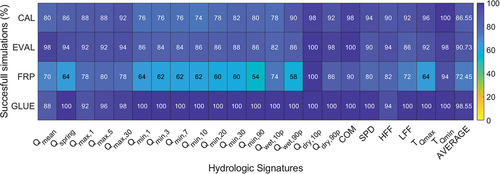
Figure 5. Model performance in reproducing distributions of the selected hydrological signatures (Table 1). Cell values are percentages of successful simulations, i.e. percentage of catchments in the calibration (CAL), evaluation (EVAL) or full record period (FRP), or percentage of the behavioural parameter sets in the Assembro catchment in the calibration period (GLUE) that well reproduced the distributions of the signatures. The last column in the heat map shows the average performance of the simulation across all signatures.

3.2.2 Evaluation of model performance in reproducing trends in hydrological signatures

Most of the selected signatures did not exhibit significant trends at the 5% level of significance according to the results of the Mann-Kendall test (Fig. 6 and Fig. S2 of the Supplementary material). Significant trends mostly emerged over the full record period (1962–2020), while they could not be detected in the two subperiods. Trends in mean and spring flows suggest that many of the selected catchments could become wetter, mainly in the north at quite high latitudes. Significant trends in annual maxima were detected in few catchments, as opposed to mostly increasing trends in annual minima detected in many catchments, particularly in the full record period. Concerning low-flow frequency (LFF), significantly increasing as well as significantly decreasing trends were detected, with a shift from decreasing trends in the northern catchments to increasing trends in the southern ones. Decreasing trends that were detected in spring pulse day (SPD) and timing of annual maxima (T_Qmax) suggest shifts in the annual runoff cycle that could be attributed to earlier snowmelt.

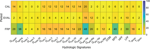
Figure 6. Percentage of catchments in which significant trends were detected in the selected hydrological signatures (Table 1) according to the results of the Mann-Kendall test in the calibration (CAL), evaluation (EVAL) and full record periods (FRP). The signatures were computed from observed flows.

Trends in the series of selected signatures (or the lack of trends) were well reproduced in most catchments in the three simulation periods (Fig. 7), according to the methodology adopted. Model performance in this regard was quite high in calibration and evaluation, with a slight decrease in the full record period, primarily in annual minima and in the wet season flow percentiles. Performance of the GLUE behavioural parameter sets in reproducing trends was exceptionally high across all signatures, including daily minima (Q_min,1) and the 10^th flow percentile in the wet season (Q_wet,90p), which is the only observed signature that exhibited a significant trend over the full record period in Assembro catchment. Low variations in performance in reproducing trends of signatures across the GLUE behavioural parameter sets suggest that equifinality in performance indicators can also imply equifinality in reproducing trends. The performance in reproducing trends was not straightforwardly related to the presence of significant trends in the observed signatures. In other words, a high percentage of catchments with significant trends in an observed signature did not imply lower performance in reproducing trends in that signature.

Figure 7. Model performance in reproducing trends in the selected hydrological signatures (Table 1). Cell values in the heat map are percentages of successful simulations, i.e. percentage of catchments in the calibration (CAL), evaluation (EVAL) or full record period (FRP), or percentage of the behavioural parameter sets in the Assembro catchment in the calibration period (GLUE) that successfully reproduced trends (or the lack of trends) in hydrological signatures. The last column in the heat map shows average performance across all signatures.

3.3 Relationships between performance indicators and hydrological signatures

3.3.1 Informativeness of performance indicators about model performance in reproducing distributions of hydrological signatures

None of the selected performance indicators alone was informative about the model ability to reproduce the distributions of all signatures across different periods (Fig. 8). At the same time, the overall informativeness varied considerably across the indicators, with noticeably lower informativeness about the signatures related to low flows. The signatures that resulted in significantly different indicator values in most cases were mean flows, annual maxima of various durations, the 90^th wet season flow percentile, and annual maxima timings, although there were significant variations in these patterns across the four simulations. Many indicators were informative about model performance in reproducing distributions of mean flows and annual maxima and minima in the three simulation periods, but these patterns could not be detected in the GLUE simulations. Such patterns included e.g. informativeness of KGE computed from daily flows and transformed flows about annual maxima and minima, respectively. The few relationships that were consistent across the four simulations include: Liu mean efficiency (LME), R² and VE, and the 90^th wet season flow percentile (Q_wet,90p), KGE computed from the entire FDC and Q_wet,90p and 30-day annual maxima, and KGE_95-100 and 20-day annual minima.

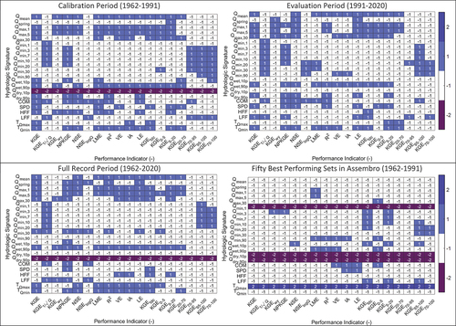
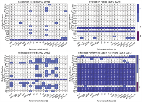
Figure 8. Informativeness of performance indicators (Table 2) about model ability to reproduce distributions of the hydrological signatures (Table 1) in different simulations. Values of 1 in the heat maps indicate that the two groups of simulations (i.e. simulations in which the distributions were well reproduced versus the remaining ones) have significantly different indicator values, suggesting that a specific indicator can be informative about model performance in reproducing the distributions. Values of −1 mean that the two groups of simulations result in similar values of an indicator, suggesting that the indicator is not informative about model ability to reproduce the distributions. A value of 2 (−2) suggests that the distributions of a signature were reproduced in all (none) of the catchments or by the behavioural parameter sets (GLUE), respectively.

Links between the performance indicators and model ability to reproduce distributions of the signatures were also examined using the Pearson correlation coefficient between the values of indicators and absolute values of WRS test statistic z. Strong negative correlations, with Pearson correlation coefficients smaller than – 0.7 (following Blasone et al. 2007), can suggest whether a specific indicator is related to model ability to reproduce distributions of a selected signature. Such correlations were detected in only a few indicators for mean annual flows in the four simulations (Fig. 9), including VE, IA, and KGE computed from the entire FDC. There were no relationships that resulted both in rejection of the WRS-2 test null hypothesis and in a correlation coefficient smaller than −0.7 across all the simulations, both of which would imply informativeness of a performance indicator about model ability to reproduce distribution of a signature.

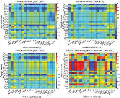
Figure 9. Pearson correlation coefficients between the values of performance indicators (Table 2) and absolute values of the Wilcoxon rank sum test statistic, z, obtained in different simulations. Strong negative correlations suggest that a specific indicator can be informative about the model ability to reproduce the distribution of a hydrological signature (Table 1), as opposed to weak negative or positive correlations.

3.3.2 Informativeness of performance indicators about model performance in reproducing trends in hydrological signatures

An initial test for autocorrelation in the data with the Box-Ljung test revealed no significant autocorrelation in the considered series of signatures. Comparisons of the simulations that properly reproduced trends in the hydrological signatures to those that did not suggest that the indicators mostly were not informative about model performance in this respect, according to the WRS-2 test (Fig. 10). However, there were differences across the simulations. For example, KGE calculated from the entire FDC (KGE_FDC) was informative about performance in reproducing trends in a few signatures in the calibration and full record periods, but not over the evaluation period. No consistent relationship between the performance indicators and model performance in reproducing the trends across the simulations was detected.

Figure 10. Informativeness of performance indicators (Table 2) about model ability to reproduce trends in series of hydrological signatures (Table 1) in different simulations. Values of 1 in the heat maps indicate that the two groups of simulations (i.e. simulations in which the trends were well reproduced versus the remaining ones) have different indicator values, which can suggest that a specific indicator is not informative about model performance in reproducing the trends. Values of −1 mean that the two groups of simulations results in similar values of a specific indicator, suggesting that a specific PI is not informative about model ability to reproduce the trends. A value of 2 (−2) suggests that the trends of a signature were reproduced in all (none) of the simulations or by the behavioural parameter sets (GLUE), respectively.

4 Discussion

The specific objectives of this research were twofold: (1) to evaluate whether hydrological models can reproduce distributions and trends in series of hydrological signatures relevant for climate change impact studies, and (2) to examine whether commonly used performance indicators can be informative about model ability to reproduce these distributions and trends. All analyses were conducted in 50 high-latitude catchments with different runoff dynamics, and over different periods to test whether potential relationships between the indicators and the model ability to reproduce the distributions or trends remain consistent. To analyse the impact of equifinality, all analyses were conducted with numerous behavioural parameter sets (Beven and Binley 1992) in one catchment.

4.1 Hydrological model: overall performance of 3DNet-Catch

On average, satisfactory values of different performance indicators were obtained across the simulations. The best performance was obtained in terms of index of agreement (IA), which is based on the absolute values of the residuals. This suggests that this indicator has a low sensitivity to discrepancies between simulated and observed flows and, as such, is not sufficiently informative about model performance. Similar conclusions were reported by Krause et al. (2005). Slightly lower performance, on average, was shown by NSE coefficients, Lindström efficiency coefficient and KGE computed from the transformed daily flows and from the highest-flow and low-flow segments of FDCs, all of which are related to model performance in extreme flows (Oudin et al. 2006, Pfannerstill et al. 2014). Values of KGE computed over the very low-flow FDC segment that was exceeded 95–100% of time (KGE_95–100) were systematically lower than KGE computed from low-flow and overall low-flow FDC segments that were exceeded 70–95% and 70–100% of time, respectively. This result shows that partitioning the low-flow segment of FDC into two subsegments (as suggested by Pfannerstill et al. 2014) contributes to a more comprehensive model evaluation.

Overall, the results demonstrated that it is challenging to achieve good performance in extreme flows, particularly in low flows during dry periods (Vaze et al. 2010, Zhang et al. 2015, Fowler et al. 2016). Poor performance over dry periods has been frequently reported in the literature, for example in studies dealing with Australian catchments affected by the Millennium drought (e.g. Thirel et al. 2015, Fowler et al. 2020, Topalović et al. 2020). No substantial differences in model performance across the three simulation periods were detected in this study, although there were significant variations in the indicators across the catchments in each simulation period, as opposed to the GLUE behavioural sets characterized by a strong equifinality. These results suggest that model suitability for CCISs should preferably be evaluated in different catchments, rather than in a single catchment with numerous parameter sets.

Variation in model performance across the catchments could not be attributed to variations in their properties in this study. As shown in Fig. 3, model performance could not be linked to e.g. catchment area, latitude, elevation or DOR (Fig. 1(c)). For example, similar performance was exhibited by catchments of various degrees of regulation, as well as in unregulated ones (e.g. catchments in the southeast of Sweden). The lack of a clear relationship between model performance and DOR can be explained by the fact that the vast majority of the selected catchments were unregulated or had rather low DOR, or that the reservoirs are managed in a way that does not considerably alter the natural runoff regime, and could be properly reproduced by the model. Slightly poorer performance was obtained in few high-elevation catchments in the northwest of Sweden, characterized by a higher percentage of snowfall and high runoff coefficients. High runoff coefficients in these catchments could be partly attributed to uncertainties in precipitation data in these regions caused by spatial interpolation from a sparse rain gauge network (Van Der Velde et al. 2013, 2014). Uncertainties in precipitation data are common, especially if precipitation occurs in the form of snowfall (Grossi et al. 2017), during high-intensity rainfall events (McMillan et al. 2011), or in high-elevation regions (Wang et al. 2016). Despite permanent development of spatial interpolation methods and processing of precipitation data, it is still a great challenge to obtain datasets of high quality and resolution (Hu et al. 2019). Consequently, high runoff coefficients are encountered in many catchments globally, such as catchments in the Pacific Northwest in the US (e.g. Addor et al. 2017). Bearing in mind the objectives of this study, a wide range of hydroclimatic regimes, ranging from snowmelt to rainfall driven, as well as those in regulated catchments, and a wide range of values of performance indicators were all essential for reaching valid conclusions on relationships between the two facets of model performance. Therefore, the collection of catchments across high-latitude climate is regarded as adequate for testing the hypotheses in this study. Nevertheless, further research is needed to thoroughly examine relationships between model performance and catchment properties (which was beyond the scope of this study), preferably with an extended collection of catchments, including those from other geographical regions with different streamflow regimes, and with other hydrological models.

4.2 Evaluation of model ability to reproduce statistical properties of hydrological signatures

Model ability to reproduce distributions and trends varied considerably across the hydrological signatures and the simulations. The lowest efficiency was obtained in reproducing distributions of signatures related to low flows (annual minima of various durations, dry-season percentiles, timings of annual minima), which was consistent with the conclusions reached from the indicator values. This was also confirmed by the fact that slightly better performance was obtained during the evaluation period than in the calibration period in reproducing distributions of annual minima (Q_min,1) and their timings (T_Qmin), as well in terms of KGE_95–100 and KGE_70–100. The model generally reproduced trends in the series quite well, irrespective of the presence of significant trends in the observed series of signatures. However, statistically significant trends were detected in, on average, six signatures in each catchment over the full record period, and in, on average, two signatures over the calibration and evaluation periods (see Figure S2 of the Supplementary material). Therefore, further research is needed to evaluate model ability to reproduce trends in the series of signatures in other catchments with more pronounced trends, such as some of the catchments presented by Thirel et al. (2015). Model transferability in terms of the indicators generally corresponded to transferability in terms of reproducing distributions and trends in the signatures.

Equifinality affected all aspects of model performance, i.e. it could be detected regardless of the approach to quantification of model performance. For example, equifinality was reflected in low variability across indicator values of different behavioural sets (e.g. VE, Fig. 4). It was also evident in model ability to reproduce distributions: for example, all behavioural sets reproduced the timings of annual maxima and most sets well reproduced distributions of annual maxima of various durations (Fig. 5). The impact of parameter equifinality was most pronounced in reproducing trends (or the lack of them) in the selected signatures (Fig. 7).

4.3 Informativeness of performance indicators about model ability to reproduce statistical properties of hydrological signatures

There were no clear and consistent relationships between the values of performance indicators and model ability to reproduce distributions or trends in series of hydrological signatures. This study was grounded on the assumption that a comparison between the indicator values of models that can reproduce the distributions, with those that cannot, can show whether specific indicators are informative about model performance in this regard, provided that such relationships remain consistent across the simulations. Few such relationships were detected in this study: for example, relationships between annual minima of various durations and KGE computed from transformed flows (KGE_1/√Q) and from very low-flow FDC segments (KGE_95–100). The relationship between distributions of annual maxima and KGE_95–100 was also confirmed by the fact that model performance in these two aspects was better in the evaluation than the calibration period in some catchments. However, these relationships do not persist in all simulations, including the simulations with the 1% best behavioural parameter sets (Fig. S3 in the Supplementary material), and simulations with the 50 best behavioural sets in the selected 50 catchments (Fig. S4). This conclusion is further supported by combined considerations of these patterns and the correlation coefficients between the indicator values and absolute z values of the WRS test statistic.

The WRS test can suggest informativeness of a certain indicator about model ability to reproduce distributions and/or trends in the series of signatures. However, this does not necessarily imply that a performance indicator that is shown to be informative about model performance in reproducing distributions of some signatures has high values, and vice versa. For example, the median values of KGE_1/√Q, KGE_70–95 and KGE_70–100 were satisfactory in the full record period, but the model failed to reproduce distributions of annual minima of varying durations, dry-season percentiles, and low-flow frequencies in most of the catchments. The discrepancies between these two aspects of model performance (i.e. performance indicators and model ability to reproduce distributions and trends) can be explained by the nature of the indicators themselves. Values of such indicators reflect differences between entire observed and simulated flow series, and are much less sensitive to differences in the distributions of series of signatures, as well as in potential underlying trends in these series. The results presented in this study clearly show that performance indicators and model ability to reproduce statistical properties of series of hydrological signatures represent two distinct facets of model performance that complement each other. Therefore, model evaluation procedures should be extended to include both aspects of model performance.

4.4 Limitations of the study and further research

The conclusions presented in this study build on the simulation results from one hydrological model in 50 high-latitude catchments. Further research is needed to repeat these analyses with other hydrological models, and in catchments in other hydroclimatic regions, and to compare those conclusions on the informativeness of performance indicators, regarding model ability to reproduce distributions and trends in the signatures, to those presented in this study. Similarly, the lists of performance indicators and hydrological signatures chosen in this study, although by no means exhaustive, could be extended in future research. Nevertheless, the timings of the 25^th and 75^th percentiles of annual runoff volume (Burn and Hag Elnur 2002, Harder et al. 2015, Melsen et al. 2018) might be excluded from such extensions, since initial analyses revealed strong autocorrelation in these series that affects the power of the Mann-Kendall test for trend (Fatichi et al. 2009, Harder et al. 2015), and since hydrological models have limited skill in reproducing them properly (Plavšić and Todorović 2018).

Most analyses conducted in this study rely on applications of the WRS test. This test was preferred for comparisons of the distributions of signatures obtained from observed and simulated flows over other suitable alternatives, such as Kolmogorov-Smirnov or Cramer-von-Mises tests (Conover 1999). Although the results from comparisons of the distributions of signatures with the Kolmogorov-Smirnov test depart from those obtained with the WRS test in up to 12% of all instances (results for the full record period), the conclusions about the informativeness of performance indicators about model ability to reproduce the distribution of the signatures corroborate those reached by using the WRS test (see Fig. S5 of the Supplementary material).

Application of the WRS test imposes certain limitations. This nonparametric test is based on a comparison of medians (Kvam and Vidakovic 2007, Kottegoda and Rosso 2008), with an underlying assumption of the WRS test that the two distributions have the same shape and variance, while other properties of series distributions, such as skewness, are not explicitly considered. Consequently, even if the series obtained from observed and simulated flows did not differ according to the WRS test, that does not mean that the quantiles computed from the two series would be equal, because quantile estimates are strongly affected by various properties of series, such as skewness or presence of outliers (Plavšić et al. 2014). Thus, further research is needed to enhance the examination of model ability to reproduce other features of hydrological signatures’ distributions. As part of such research, application of different, complementary statistical tests can be considered.

Climate change impact on floods poses a great concern and a great challenge to CCISs. Models’ ability to accurately simulate the highest flows, such as annual maxima, is generally limited (Brunner et al. 2021). To improve model skill in reproducing annual maxima, Mizukami et al. (2019) proposed the annual peak flow bias (APFB) metric as objective function. Although specifically tailored for annual maxima, this performance indicator cannot be considered informative about model ability to reproduce their distributions, according to the methodology adopted in this study (see Fig. S6 in the Supplementary material). The same conclusions were reached for the mean flows and annual daily minima. These results once again highlighted issues with reproducing the most extreme flows, and the need for further research in this regard. Furthermore, spring floods triggered by snowmelt have different statistical properties than rainfall-induced summer or autumn floods; thus, these two series should be analysed independently (Blazkova and Beven 2009). The peak over threshold method can also be used for flood flow quantile estimation (Plavšić 2005, Todorović et al. 2017, Tabari 2021).

Gelfan and Millionshchikova (2018) state that: “in order not to get lost in the ‘jungle of models,’ one needs to be able to distinguish between models appropriate for impact studies and unsuitable ones,” and emphasize that “there are a lot of ‘good’ models that pretend to be suitable for impact studies, and the number of such models grows like a snowball.” The approach applied in this paper is in line with the appeals of the hydrological community for novel evaluation procedures aimed at identifying models suitable for CCISs that can potentially mitigate uncertainty in hydrological projections under climate change (Fowler et al. 2018b). This study clearly shows that commonly used performance indicators fail to show model performance in reproducing statistical properties of series of hydrological signatures that climate change impact assessments build on. In other words, good model performance in terms of commonly used indicators does not warrant that the statistical properties of signatures are well reproduced, which can eventually result in misleading assessment of climate change impacts and failure in the identification of optimal adaptation strategies. This study presented an evaluation of the performance of hydrological models that are run with the observed climatic series, while hydrological series in CCISs would inevitably be affected by uncertainties in climate projections. However, it is essential to establish robust evaluation procedures that can identify hydrological models suitable for CCISs under current conditions, with observed data that allow comparisons of observed and simulated variables. The application of the WRS test to evaluate model performance in reproducing distributions of the selected signatures represents a step forward in this direction.

5 Conclusions

Climate change adaptation strategies are grounded in statistical analyses of the series of hydrological regime features (i.e. hydrological signatures), such as mean or extreme flows, or extreme flow timings and durations. Therefore, distributions and trends in series of hydrological signatures should be accurately reproduced by hydrological models. Although crucial for climate change impact studies (CCISs), this aspect of hydrological model performance is rarely analysed. In this paper, we provided novel insights on model performance and suitability for climate change impact studies by: (1) thoroughly evaluating model ability to reproduce distributions and trends in series of hydrological signatures relevant for CCISs, and (2) examining whether commonly used performance indicators are informative about how well a model can reproduce these distribution and trend properties.

The simulations with the 3DNet-Catch model for 50 high-latitude catchments in Sweden revealed considerable differences in the model performance. Specifically, distributions of low-flow signatures generally were not well reproduced, while model performance for high-flow-related signatures was noticeably better. Such behaviour was also exhibited by the performance indicators. However, no strong, clear, and consistent relationships between the values of indicators, and model performance in reproducing the distributions and trends in the signatures, were detected in this study. This means that good model performance in terms of the commonly used performance indicators cannot warrant that the distributions or trends in the series of signatures are well reproduced, and vice versa. This clearly shows that these two facets of model performance are distinct and complementary, and that model suitability for CCISs cannot be appraised merely using performance indicators. Therefore, traditional model evaluations based merely on performance indicators should be extended, and evaluation focused on distributions and trends in signatures presented in this paper can be considered a part of these efforts. Model performance in reproducing distributions cannot be used straightforwardly as an OF for model calibration; however, it can be included in a process of model selection for CCISs and, thereby, potentially reduce uncertainties in the flow projections under climate change due to model equifinality.

Acknowledgements

This research is conducted as part of the project “Reducing uncertainties in hydrological climate change impact research to allow for robust streamflow simulations” supported by the Swedish Research Council (VR starting grant: 2017-04970). The data used in this paper were obtained from the Swedish Meteorological and Hydrological Institute (SMHI). The authors thank Prof. Miloš Stanić from the University of Belgrade for his help with setting up the 3DNet-Catch model, and the two anonymous reviewers for helpful and constructive comments.

Disclosure statement

No potential conflict of interest was reported by the authors.

Supplementary material

Supplemental data for this article can be accessed online at https://doi.org/10.1080/02626667.2022.2104646

Data availability statement

Hydro-climatic data can be retrieved from the Swedish Meteorological and Hydrological Institute (SMHI) database (http://vattenwebb.smhi.se/). Geospatial data for the streamflow stations can be downloaded from the SMHI SVAR database (https://www.smhi.se/publikationer/svar-svenskt-vattenarkiv-1.17833).

Additional information

Funding

This work was supported by the Vetenskapsrådet [2017-04970].

References

- Addor, N., et al., 2014. Robust changes and sources of uncertainty in the projected hydrological regimes of Swiss catchments. Water Resources Research, 50 (10), 7541–7562. doi:10.1002/2014WR015549
- Addor, N., et al., 2017. The CAMELS data set: catchment attributes and meteorology for large-sample studies. Hydrology and Earth System Science, 21 (10), 5293–5313. doi:10.5194/hess-21-5293-2017
- Addor, N. and Melsen, L.A., 2019. Legacy, rather than adequacy, drives the selection of hydrological models. Water Resources Research, 55 (1), 378–390. doi:10.1029/2018WR022958
- Asadzadeh, M., Tolson, B.A., and Burn, D.H., 2014. A new selection metric for multiobjective hydrologic model calibration. Water Resources Research, 50 (9), 7082–7099. doi:10.1002/2013WR014970
- Bastola, S., Murphy, C., and Sweeney, J., 2011. The role of hydrological modelling uncertainties in climate change impact assessments of Irish river catchments. Advances in Water Resources, 34 (5), 562–576. doi:10.1016/j.advwatres.2011.01.008
- Beck, H.E., et al., 2017. Global evaluation of runoff from 10 state-of-the-art hydrological models. Hydrology and Earth System Sciences, 21 (6), 2881–2903. doi:10.5194/hess-21-2881-2017
- Bergström, S., et al., 2001. Climate change impacts on runoff in Sweden-assessments by global climate models, dynamical downscaling and hydrological modelling. Climate Research, 16 (2), 101–112. doi:10.3354/cr016101
- Beven, K. and Binley, A., 1992. The future of distributed models: model calibration and uncertainty prediction. Hydrological Processes, 6 (3), 279–298. doi:10.1002/hyp.3360060305
- Blasone, R.-S., Madsen, H., and Rosbjerg, D., 2007. Parameter estimation in distributed hydrological modelling: comparison of global and local optimisation techniques. Nordic Hydrology, 38 (4–5), 451. doi:10.2166/nh.2007.024
- Blazkova, S. and Beven, K., 2009. A limits of acceptability approach to model evaluation and uncertainty estimation in flood frequency estimation by continuous simulation: skalka catchment, Czech Republic. Water Resources Research, 45 (12), 1–12. doi:10.1029/2007WR006726
- Blöschl, G., et al., 2017. Changing climate shifts timing of European floods. Science, 357 (6351), 588–590. doi:10.1126/science.aan2506
- Blöschl, G., et al., 2019a. Twenty-three unsolved problems in hydrology (UPH) – a community perspective. Hydrological Sciences Journal, 64 (10), 1141–1158. doi:10.1080/02626667.2019.1620507
- Blöschl, G., et al., 2019b. Changing climate both increases and decreases European river floods. Nature, 573 (7772), 108–111. doi:10.1038/s41586-019-1495-6
- Blöschl, G., and Montanari, A., 2010. Climate change impacts—throwing the dice? Hydrological Processes, 381 (3), 374–381. doi:10.1002/hyp.7574
- Booij, M.J., 2005. Impact of climate change on river flooding assessed with different spatial model resolutions. Journal of Hydrology, 303 (1–4), 176–198. doi:10.1016/j.jhydrol.2004.07.013
- Bosshard, T., et al., 2013. Quantifying uncertainty sources in an ensemble of hydrological climate-impact projections. Water Resources Research, 49 (3), 1523–1536. doi:10.1029/2011WR011533
- Brooks, R. and Corey, A., 1964. Hydraulic properties of porous media. Hydrology Papers, Colorado State University, Fort Collins: Colorado State University. Available from: http://www.citeulike.org/group/1336/article/711012
- Brunner, M.I., et al., 2021. Flood spatial coherence, triggers, and performance in hydrological simulations: large-sample evaluation of four streamflow-calibrated models. Hydrology and Earth System Sciences, 25 (1), 105–119. doi:10.5194/hess-25-105-2021
- Bum Kim, K., Kwon, H.-H., and Han, D., 2021. Bias-correction schemes for calibrated flow in a conceptual hydrological model. Hydrology Research, 196–211. doi:10.2166/nh.2021.043
- Burn, D.H. and Hag Elnur, M.A., 2002. Detection of hydrologic trends and variability. Journal of Hydrology, 255 (1–4), 107–122. doi:10.1016/S0022-1694(01)00514-5
- Carlisle, D.M., et al., 2017. Biological relevance of streamflow metrics: regional and national perspectives. Freshwater Science, 36 (4), 927–940. doi:10.1086/694913
- Cayan, D.R., et al. 2001. Changes in the onset of spring in the Wesetern United States. Bulletin of the American Meteorological Society, 82 (3), 2265–2266. doi:10.1175/1520-0477(2001)082<0399:CITOOS>2.3.CO;2
- Chen, J., et al., 2017. Impacts of weighting climate models for hydro-meteorological climate change studies. Journal of Hydrology, 549, 534–546. doi:10.1016/j.jhydrol.2017.04.025
- Chen, J., Brissette, F.P., and Lucas-Picher, P., 2016. Transferability of optimally-selected climate models in the quantification of climate change impacts on hydrology. Climate Dynamics, 47 (9–10), 3359–3372. doi:10.1007/s00382-016-3030-x
- Chen, Y.R. and Yu, B., 2016. Impact assessment of climatic and land-use changes on flood runoff in southeast Queensland. Water and Energy International, 58RNI (12), 80. doi:10.1080/02626667.2014.945938
- Chiew, F.H.S., Zheng, H., and Vaze, J., 2015. Implication of calibration period on modelling climate change impact on future runoff. IAHS Symposium HS02, 26th General Assembly of the International Union of Geodesy and Geophysics, Prague, Czech Republic, 22 June–2 July 2015, 371, 3–6. doi:10.5194/piahs-371-3-2015
- Coffey, M.E., et al., 2004. Statistical procedures for evaluating daily and monthly hydrologic model predictions. Transactions of the ASAE, 47 (1), 59–68. doi:10.13031/2013.15870
- Conover, W.J., 1999. Practical nonparametric statistics. 3rd ed. New York: John Wiley & Sons, inc.
- CORINE Land Cover, 2012. Copernicus. Available from: https://land.copernicus.eu/pan-european/corine-land-cover/clc-2012?tab=mapview
- Coron, L., et al., 2012. Crash testing hydrological models in contrasted climate conditions: an experiment on 216 Australian catchments. Water Resources Research, 48 (5), W05552, 1–17. doi:10.1029/2011WR011721
- Criss, R.E. and Winston, W.E., 2008. Do Nash values have value ? Discussion and alternate proposals. Hydrological Processes, 22 (14), 2723–2725. doi:10.1002/hyp
- Crochemore, L., et al., 2015. Comparing expert judgement and numerical criteria for hydrograph evaluation. Hydrological Sciences Journal, 60 (3), 402–423. doi:10.1080/02626667.2014.903331
- Cunderlik, J.M. and Ouarda, T.B.M.J., 2009. Trends in the timing and magnitude of floods in Canada. Journal of Hydrology, 375 (3–4), 471–480. doi:10.1016/j.jhydrol.2009.06.050
- Dams, J., et al., 2015. Multi-model approach to assess the impact of climate change on runoff. Journal of Hydrology, 529, 1601–1616. doi:10.1016/j.jhydrol.2015.08.023
- Dankers, R., et al., 2014. First look at changes in flood hazard in the inter-sectoral impact model intercomparison project ensemble. Proceedings of the National Academy of Sciences, 111 (9), 3257–3261. doi:10.1073/pnas.1302078110
- Dankers, R. and Feyen, L., 2009. Flood hazard in Europe in an ensemble of regional climate scenarios. Journal of Geophysical Research, 114 (D16), D16108. doi:10.1029/2008JD011523
- Daraio, J.A., 2020. Hydrologic model evaluation and assessment of projected climate change impacts using bias-corrected stream flows. Water, 12 (8), 2312. doi:10.3390/w12082312
- Eisner, S., et al., 2017. An ensemble analysis of climate change impacts on streamflow seasonality across 11 large river basins. Climatic Change, 141 (3), 401–417. doi:10.1007/s10584-016-1844-5
- Eklund, A., 2011. SVAR, Svenskt vattenarkiv (No. 53). Norrköping, Sweden. Available from: https://www.smhi.se/publikationer/svar-svenskt-vattenarkiv-1.17833
- Euser, T., et al., 2013. A framework to assess the realism of model structures using hydrological signatures. Hydrology and Earth System Sciences, 17 (5), 1893–1912. doi:10.5194/hess-17-1893-2013
- Farmer, W.H., Over, T.M., and Kiang, J.E., 2018. Bias correction of simulated historical daily streamflow at ungauged locations by using independently estimated flow duration curves. Hydrology and Earth System Sciences, 22 (11), 5741–5758. doi:10.5194/hess-22-5741-2018
- Fatichi, S., et al., 2009. Deterministic versus stochastic trends: detection and challenges. Journal of Geophysical Research, 114 (D18), 1–11. doi:10.1029/2009JD011960
- Feng, D. and Beighley, E., 2020. Identifying uncertainties in hydrologic fluxes and seasonality from hydrologic model components for climate change impact assessments. Hydrology and Earth System Sciences, 24 (5), 2253–2267. doi:10.5194/hess-24-2253-2020
- Fenicia, F., et al., 2007. Soft combination of local models in a multi-objective framework. Hydrology and Earth System Sciences, 11 (6), 275–301. Available from: www.hydrol-earth-syst-sci.net/11/1797/2007/
- Fowler, K., et al., 2018a. Improved rainfall-runoff calibration for drying climate: choice of objective function. Water Resources Research, 54 (5), 3392–3408. doi:10.1029/2017WR022466
- Fowler, K., et al., 2018b. Simulating runoff under changing climatic conditions: a framework for model improvement. Water Resources Research, 54 (12), 9812–9832. doi:10.1029/2018WR023989
- Fowler, K., et al., 2020. Many commonly used rainfall‐runoff models lack long, slow dynamics: implications for runoff projections. Water Resources Research, 56 (5), 1–27. doi:10.1029/2019WR025286
- Fowler, K.J.A., et al., 2016. Simulating runoff under changing climatic conditions: revisiting an apparent deficiency of conceptual rainfall-runoff models. Water Resources Research, 52 (3), 1820–1846. doi:10.1002/2015WR018068
- Gain, A.K., et al., 2013. Thresholds of hydrologic flow regime of a river and investigation of climate change impact—the case of the Lower Brahmaputra river Basin. Climatic Change, 120 (1–2), 463–475. doi:10.1007/s10584-013-0800-x
- Gangrade, S., Kao, S.-C., and McManamay, R.A., 2020. Multi-model hydroclimate projections for the Alabama-Coosa-Tallapoosa River Basin in the Southeastern United States. Scientific Reports, 10 (1), 2870. doi:10.1038/s41598-020-59806-6
- García-Portugués, E., 2022. Notes for nonparametric statistics [WWW Document]. Version 6.5.7. URL. Available from: https://bookdown.org/egarpor/NP-UC3M/ [ Accessed 19 April 2022].
- Garcia, F., Folton, N., and Oudin, L., 2017. Which objective function to calibrate rainfall–runoff models for low-flow index simulations? Hydrological Sciences Journal, 62 (7), 1149–1166. doi:10.1080/02626667.2017.1308511
- Gelfan, A., et al., 2020. Does a successful comprehensive evaluation increase confidence in a hydrological model intended for climate impact assessment? Climatic Change, 163 (3), 1165–1185. doi:10.1007/s10584-020-02930-z
- Gelfan, A.N. and Millionshchikova, T.D., 2018. Validation of a hydrological model intended for impact study: problem statement and solution example for Selenga River Basin. Water Resources, 45 (S1), 90–101. doi:10.1134/S0097807818050354
- Girons Lopez, M., Crochemore, L., and Pechlivanidis, I.G., 2021. Benchmarking an operational hydrological model for providing seasonal forecasts in Sweden. Hydrology and Earth System Sciences, 25 (3), 1189–1209. doi:10.5194/hess-25-1189-2021
- González-Zeas, D., et al., 2012. Improving runoff estimates from regional climate models: a performance analysis in Spain. Hydrology and Earth System Sciences, 16 (6), 1709–1723. doi:10.5194/hess-16-1709-2012
- Gosling, S.N., et al., 2017. A comparison of changes in river runoff from multiple global and catchment-scale hydrological models under global warming scenarios of 1 °C, 2 °C and 3 °C. Climatic Change, 141 (3), 577–595. doi:10.1007/s10584-016-1773-3
- Grossi, G., et al., 2017. Snow precipitation measured by Gauges: systematic error estimation and data series correction in the Central Italian Alps. Water, 9 (7), 461. doi:10.3390/w9070461
- Gudmundsson, L., et al., 2012. Comparing large-scale hydrological model simulations to observed runoff percentiles in Europe. Journal of Hydrometeorology, 13 (2), 604–620. doi:10.1175/JHM-D-11-083.1
- Gupta, H.V., et al., 2009. Decomposition of the mean squared error and NSE performance criteria: implications for improving hydrological modelling. Journal of Hydrology, 377 (1–2), 80–91. doi:10.1016/j.jhydrol.2009.08.003
- Hakala, K., et al., February 2019. Hydrological modeling of climate change impacts. Encyclopedia of Water, 1–20. doi:10.1002/9781119300762.wsts0062
- Hamon, W.R., 1961. Estimating potential evaporation. Proceedings of the American Society of Civil Engineers, Journal of the Hydraulic Divison, 87 (HY3), 107–120.
- Hannaford, J., et al., 2013. The influence of decadal-scale variability on trends in long European streamflow records. Hydrology and Earth System Sciences, 17 (7), 2717–2733. doi:10.5194/hess-17-2717-2013
- Harder, P., Pomeroy, J.W., and Westbrook, C.J., 2015. Hydrological resilience of a Canadian Rockies headwaters basin subject to changing climate, extreme weather, and forest management. Hydrological Processes, 29 (18), 3905–3924. doi:10.1002/hyp.10596
- Hattermann, F.F., et al., 2017. Cross‐scale intercomparison of climate change impacts simulated by regional and global hydrological models in eleven large river basins. Climatic Change, 141 (3), 561–576. doi:10.1007/s10584-016-1829-4
- Henestål, J., et al., 2012. Arbete med SVAR version 2012_1 och 2012_2, Svenskt Vattenarkiv, en databas vid SMHI. DM #154591.
- Hoang, L.P., et al., 2016. Mekong River flow and hydrological extremes under climate change. Hydrology and Earth System Sciences, 20 (7), 3027–3041. doi:10.5194/hess-20-3027-2016
- Hu, Q., et al., 2019. Rainfall spatial estimations: a review from spatial interpolation to multi-source data merging. Water, 11 (3), 579. doi:10.3390/w11030579
- Huang, S., et al., 2020. Impacts of hydrological model calibration on projected hydrological changes under climate change—a multi-model assessment in three large river basins. Climatic Change, 163 (3), 1143–1164. doi:10.1007/s10584-020-02872-6
- Johansson, B., 2000. Areal precipitation and temperature in the Swedish mountains. Hydrology Research, 31 (3), 207–228. doi:10.2166/nh.2000.0013
- Joseph, J., et al., 2018. Hydrologic impacts of climate change: comparisons between hydrological parameter uncertainty and climate model uncertainty. Journal of Hydrology, 566 (July), 1–22. doi:10.1016/j.jhydrol.2018.08.080
- Karlsson, I.B., et al., 2016. Combined effects of climate models, hydrological model structures and land use scenarios on hydrological impacts of climate change. Journal of Hydrology, 535, 301–317. doi:10.1016/j.jhydrol.2016.01.069
- Kay, A.L., et al., 2009. Comparison of uncertainty sources for climate change impacts: flood frequency in England. Climatic Change, 92 (1–2), 41–63. doi:10.1007/s10584-008-9471-4
- Kendall, M.G., 1938. A new measure of rank correlation. Biometrika, 30 (1/2), 81. doi:10.2307/2332226
- Keramat, M. and Kielbasa, R., 1997. Latin hypercube sampling Monte Carlo estimation of average quality index for integrated circuits. Analog Integrated Circuits And Signal Processing, 1–2 (1/2), 131–142. doi:10.1023/A:1008207113480
- Kiesel, J., et al., 2020. Streamflow-based evaluation of climate model sub-selection methods. Climatic Change, 163 (3), 1267–1285. doi:10.1007/s10584-020-02854-8
- Kirchner, J.W., 2006. Getting the right answers for the right reasons: linking measurements, analyses, and models to advance the science of hydrology. Water Resources Research, 42 (3), W03S04, 1–5. doi:10.1029/2005WR004362
- Klemeš, V., 1986. Operational testing of hydrological simulation models. Hydrological Sciences, 31 (1), 13–24. doi:10.1080/02626668609491024
- Kormos, P.R., et al., 2016. Trends and sensitivities of low streamflow extremes to discharge timing and magnitude in Pacific Northwest mountain streams. Water Resources Research, 52 (7), 4990–5007. doi:10.1002/2015WR018125
- Kottegoda, N.T. and Rosso, R., 2008. Applied statistics for civil and environmental engineers. Second Edi. Oxford, United Kingdom: Blackwell Publishing.
- Kottek, M., et al., 2006. World map of the Köppen-Geiger climate classification updated. Meteorologische Zeitschrift, 15 (3), 259–263. doi:10.1127/0941-2948/2006/0130
- Krause, P., Boyle, D.P., and Bäse, F., January 2005. Comparison of different efficiency criteria for hydrological model assessment. Advances in Geosciences, 5, 89–97. doi:10.5194/adgeo-5-89-2005
- Krysanova, V., et al., 2017. Intercomparison of regional-scale hydrological models and climate change impacts projected for 12 large river basins worldwide—a synthesis. Environmental Research Letters, 12 (10), 105002. doi:10.1088/1748-9326/aa8359
- Krysanova, V., et al., 2018. How the performance of hydrological models relates to credibility of projections under climate change. Hydrological Sciences Journal, 63 (5), 696–720. doi:10.1080/02626667.2018.1446214
- Kvam, P.H. and Vidakovic, B., 2007. Nonparametric statistics with applications to science and engineering. New Jersey: Wiley-interscience.
- Legates, D.R. and McCabe, G.J., 1999. Evaluating the use of “goodness-of-fit” measures in hydrologic and hydroclimatic model validation. Water Resources Research, 35 (1), 233–241. doi:10.1029/1998WR900018
- Lehner, B., et al., 2006. Estimating the impact of global change on flood and drought risks in Europe: a continental, integrated analysis. Climatic Change, 75 (3), 273–299. doi:10.1007/s10584-006-6338-4
- Lespinas, F., Ludwig, W., and Heussner, S., April 2014. Hydrological and climatic uncertainties associated with modeling the impact of climate change on water resources of small Mediterranean coastal rivers. Journal of Hydrology, 511, 403–422. doi:10.1016/j.jhydrol.2014.01.033
- Liu, D., August 2020. A rational performance criterion for hydrological model. Journal of Hydrology, 590, 125488. doi:10.1016/j.jhydrol.2020.125488
- Ljung, G. and Box, G., 1978. On a measure of lack of fit in time series models. Biometrika, 65 (2), 297–303. doi:10.2307/2335207
- Ludwig, R., et al., 2009. The role of hydrological model complexity and uncertainty in climate change impact assessment. Advances in Geosciences, 21, 63–71. doi:10.5194/adgeo-21-63-2009
- Mann, H.B., 1945. Nonparametric Tests Against Trend. Econometrica, 13 (3), 245. doi:10.2307/1907187
- Maurer, E.P., Brekke, L.D., and Pruitt, T., 2010. Contrasting lumped and distributed hydrology models for estimating climate change impacts on California watersheds. JAWRA Journal of the American Water Resources Association, 46 (5), 1024–1035. doi:10.1111/j.1752-1688.2010.00473.x
- McMillan, H., et al., 2011. Rainfall uncertainty in hydrological modelling: an evaluation of multiplicative error models. Journal of Hydrology, 400 (1–2), 83–94. doi:10.1016/j.jhydrol.2011.01.026
- McMillan, H.K., 2021. A review of hydrologic signatures and their applications. WIREs Water, 8 (1). doi:10.1002/wat2.1499
- Melsen, L.A., et al., 2018. Mapping (dis)agreement in hydrologic projections. Hydrology and Earth System Sciences, 22 (3), 1775–1791. doi:10.5194/hess-22-1775-2018
- Mendoza, P.A., et al., 2015. Effects of hydrologic model choice and calibration on the portrayal of climate change impacts. Journal of Hydrometeorology, 16 (2), 762–780. doi:10.1175/JHM-D-14-0104.1
- Mendoza, P.A., et al., 2016. How do hydrologic modeling decisions affect the portrayal of climate change impacts? Hydrological Processes, 30 (7), 1071–1095. doi:10.1002/hyp.10684
- Minville, M., Brissette, F., and Leconte, R., 2008. Uncertainty of the impact of climate change on the hydrology of a nordic watershed. Journal of Hydrology, 358 (1–2), 70–83. doi:10.1016/j.jhydrol.2008.05.033
- Mishra, S.K. and Singh, V.P., 2003. SCS-CN method. In: Soil conservation service curve number (SCS-CN) methodology. Water Scie. Dordrecht, 84–146. doi:10.1007/978-94-017-0147-1_2
- Mishra, V., et al., 2020. Does comprehensive evaluation of hydrological models influence projected changes of mean and high flows in the Godavari River basin? Climatic Change, 163 (3), 1187–1205. doi:10.1007/s10584-020-02847-7
- Mizukami, N., et al., 2019. On the choice of calibration metrics for “high-flow” estimation using hydrologic models. Hydrology and Earth System Sciences, 23 (6), 2601–2614. doi:10.5194/hess-23-2601-2019
- Montgomery, D.C. and Runger, G.C., 2003. Applied statistics and probability for engineers. 3rd ed. New York: John Wiley & Sons.
- Motavita, D.F., et al., 2019. The comprehensive differential split-sample test: a stress-test for hydrological model robustness under climate variability. Journal of Hydrology, 573 (March), 501–515. doi:10.1016/j.jhydrol.2019.03.054
- Najafi, M.R., Moradkhani, H., and Jung, I.W., 2011. Assessing the uncertainties of hydrologic model selection in climate change impact studies. Hydrological Processes, 25 (18), 2814–2826. doi:10.1002/hyp.8043
- Nash, J.E. and Sutcliffe, J.V., 1970. River flow forecasting through conceptual models, Part I - A discussion of principles. Journal of Hydrology, 10 (3), 282–290. doi:10.1016/0022-1694(70)90255-6
- Nicolle, P., et al., 2014. Benchmarking hydrological models for low-flow simulation and forecasting on French catchments. Hydrology and Earth System Sciences, 18 (8), 2829–2857. doi:10.5194/hess-18-2829-2014
- Olden, J.D. and Poff, N.L., 2003. Redundancy and the choice of hydrologic indices for characterizing streamflow regimes. River Research and Applications, 19 (2), 101–121. doi:10.1002/rra.700
- Olsson, J., et al., 2016. Hydrological climate change impact assessment at small and large scales: key messages from recent progress in Sweden. Climate, 4 (3), 39. doi:10.3390/cli4030039
- Osuch, M., et al. August 2016. Projected changes in flood indices in selected catchments in Poland in the 21st century. Stochastic Environmental Research and Risk Assessment, 18, 1–23. doi:10.1007/s00477-016-1296-5
- Oudin, L., et al., 2006. Dynamic averaging of rainfall-runoff model simulations from complementary model parameterizations. Water Resources Research, 42 (7), W07410, 1–10. doi:10.1029/2005WR004636
- Parajka, J., et al., 2016. Uncertainty contributions to low flow projections in Austria. Hydrology and Earth System Sciences, 20 (5), 2085–2101. doi:10.5194/hess-20-2085-2016
- Pechlivanidis, I.G.G., et al., 2016. Analysis of hydrological extremes at different hydro-climatic regimes under present and future conditions. Climatic Change, 141 (3), 467–481. doi:10.1007/s10584-016-1723-0
- Peel, M.C. and Blöschl, G., 2011. Hydrological modelling in a changing world. Progress in Physical Geography, 35 (2), 249–261. doi:10.1177/0309133311402550
- Pfannerstill, M., Guse, B., and Fohrer, N., 2014. Smart low flow signature metrics for an improved overall performance evaluation of hydrological models. Journal of Hydrology, 510, 447–458. doi:10.1016/j.jhydrol.2013.12.044
- Plavšić, J., 2005. Analiza rizika od poplava pomoću prekidnih slučajnih procesa. Belgrade, Serbia: Univerzitet u Beogradu.
- Plavšić, J., Mihailović, V., and Blagojević, B., 2014. Assessment of methods for outlier detection and. In: E. Ferrari ed. Proceedings of the Mediterranean Meeting on ″Monitoring, modelling and early warning of extreme events triggered by heavy rainfalls″. Cosenza, Italy: University of Calabria, 181–192.
- Plavšić, J. and Todorović, A., 2018. Accuracy of runoff timing in simulations with the hydrologic models. In: M.T. Bešević, I.M. Miličić, and O. Gabrić, eds. ZBORNIK RADOVA 6. MEĐUNARODNE KONFERENCIJE SAVREMENA DOSTIGNUĆA U GRAĐEVINARSTVU 2018. SUbotica, Serbia: Faculty of Civil ENgineering, 373–382. doi:10.14415/konferencijaGFS2018
- Pokhrel, Y., et al., 2021. Global terrestrial water storage and drought severity under climate change. Nature Climate Change, 11 (3), 226–233. doi:10.1038/s41558-020-00972-w
- Pool, S., Vis, M., and Seibert, J., 2018. Evaluating model performance: towards a non-parametric variant of the Kling-Gupta efficiency. Hydrological Sciences Journal, 63 (13–14), 1941–1953. doi:10.1080/02626667.2018.1552002
- Potter, N.J., Chiew, F.H.S., and Frost, A.J., 2010. An assessment of the severity of recent reductions in rainfall and runoff in the Murray–Darling Basin. Journal of Hydrology, 381 (1–2), 52–64. doi:10.1016/j.jhydrol.2009.11.025
- Prudhomme, C. and Davies, H., 2009a. Assessing uncertainties in climate change impact analyses on the river flow regimes in the UK. Part 1: baseline climate. Climatic Change, 93 (1), 177–195. doi:10.1007/s10584-008-9464-3
- Prudhomme, C. and Davies, H., 2009b. Assessing uncertainties in climate change impact analyses on the river flow regimes in the UK. Part 2: future climate. Climatic Change, 93 (1–2), 197–222. doi:10.1007/s10584-008-9461-6
- Refsgaard, J.C., et al., 2014. A framework for testing the ability of models to project climate change and its impacts. Climatic Change, 122 (1), 271–282. doi:10.1007/s10584-013-0990-2
- Ricard, S., Sylvain, J.D., and Anctil, F., 2019. Exploring an alternative configuration of the hydroclimatic modeling Chain, based on the notion of asynchronous objective functions. Water (Switzerland), 11 (10). doi:10.3390/w11102012
- Ricard, S., Sylvain, J.-D., and Anctil, F., October 2020. Asynchronous hydroclimatic modeling for the construction of physically based streamflow projections in a context of observation scarcity. Frontiers in Earth Science, 8, 1–16. doi:10.3389/feart.2020.556781
- Richter, B.D., et al., 1996. A method for assessing hydrologic alteration within ecosystems. Conservation Biology, 10 (4), 1163–1174. Available from: http://links.jstor.org/sici?sici=OSSS-8892%28199608%2910%3A4%3C1163%3AAMFAHA%3E2.0.C0%3B2-E.
- Roudier, P., et al., 2016. Projections of future floods and hydrological droughts in Europe under a +2°C global warming. Climatic Change, 135 (2), 341–355. doi:10.1007/s10584-015-1570-4
- Santos, L., Thirel, G., and Perrin, C., June 2018. Technical note: pitfalls in using log-transformed flows within the KGE criterion. Hydrology and Earth System Sciences Discussions, 1–14. doi:10.5194/hess-2018-298
- Schaefli, B., et al., 2014. SEHR-ECHO v1.0: a spatially explicit hydrologic response model for ecohydrologic applications. Geoscientific Model Development, 7 (6), 2733–2746. doi:10.5194/gmd-7-2733-2014
- Schewe, J., et al., 2014. Multimodel assessment of water scarcity under climate change. Proceedings of the National Academy of Sciences, 111 (9), 3245–3250. doi:10.1073/pnas.1222460110
- Seibert, J., 2003. Reliability of model predictions outside calibration conditions. Hydrology Research, 34 (5), 477–492. doi:10.2166/nh.2003.0019
- Seibert, J. and Vis, M.J.P., 2010. HBV-lightHELP. Available from: http://www.geo.uzh.ch/en/units/h2k/services/hbv-model
- Seiller, G., Roy, R., and Anctil, F., 2017. Influence of three common calibration metrics on the diagnosis of climate change impacts on water resources. Journal of Hydrology, 547, 280–295. doi:10.1016/j.jhydrol.2017.02.004
- Sen, P.K., 1968. Estimates of the regression coefficient based on Kendall’s Tau. Journal of the American Statistical Association, 63 (324), 1379. doi:10.2307/2285891
- Shafii, M. and Tolson, B.A., 2015. Optimizing hydrological consistency by incorporating hydrological signatures into model calibration objectives. Water Resources Research, 51 (5), 3796–3814. doi:10.1002/2014WR016520
- SLU, 2015. Rödlistade arter i Sverige 2015. Edited by A. Westling, Uppsala, Sweden: Sveriges lantbruksuniversitet (Swedish University of Agricultural Sciences). Available from: http://urn.kb.se/resolve?urn=urn:nbn:se:slu:epsilon-e-3658
- SMHI, 2005. PTHBV klimatdatabas för hydrologiska beräkningar [PTHBV climate database for hydrological calculations] (Produktblad). Norrköping, Sweden. Available from: https://www.smhi.se/polopoly_fs/1.166963!/PTHBV_produktblad DM19775.pdf [Accessed 15 Aug 2022].
- Stanić, M., et al., 2018. Extreme flood reconstruction by using the 3DNet platform for hydrological modelling. Journal of Hydroinformatics, 20 (4). doi:10.2166/hydro.2017.050
- Stewart, I.T., Cayan, D.R., and Dettinger, M.D., 2005. Changes toward earlier streamflow timing across Western North America. Journal of Climate, 18 (8), 1136–1155. doi:10.1175/JCLI3321.1
- Tabari, H., 2021. Extreme value analysis dilemma for climate change impact assessment on global flood and extreme precipitation. Journal of Hydrology, 593, 125932. doi:10.1016/j.jhydrol.2020.125932 [August 2020].
- Teng, J., et al., 2012. Estimating the relative uncertainties sourced from GCMs and hydrological models in modeling climate change impact on runoff. Journal of Hydrometeorology, 13 (1), 122–139. doi:10.1175/JHM-D-11-058.1
- Teutschbein, C. and Seibert, J., 2010. Regional climate models for hydrological impact studies at the catchment scale: a review of recent modeling strategies. Geography Compass, 4 (7), 834–860. doi:10.1111/j.1749-8198.2010.00357.x
- Teutschbein, C., et al., 2018. Simulating streamflow in ungauged basins under a changing climate: the importance of landscape characteristics. Journal of Hydrology, 561, 160–178. Available from: https://doi.org/10/gdx3db
- Teutschbein, C. and Seibert, J., 2012. Bias correction of regional climate model simulations for hydrological climate-change impact studies: review and evaluation of different methods. Journal of Hydrology, 456–457, 12–29. doi:10.1016/j.jhydrol.2012.05.052
- Teutschbein, C. and Seibert, J., 2013. Is bias correction of regional climate model (RCM) simulations possible for non-stationary conditions? Hydrology and Earth System Sciences, 17 (12), 5061–5077. doi:10.5194/hess-17-5061-2013
- Thirel, G., et al., 2015. Hydrology under change: an evaluation protocol to investigate how hydrological models deal with changing catchments. Hydrological Sciences Journal, 60 (7–8), 1184–1199. doi:10.1080/02626667.2014.967248
- Todorović, A., et al., 2017. Assessment of climate change impact on floods in two catchments in Serbia. In Conference proceedings 5th International Conference Contemporary Achievements in Civil Engineering 2017. Subotica, Serbia: Faculty of Civil Engineering Subotica, 685–694. Available from: http://www.gf.uns.ac.rs/~konferencija/radovi.php
- Todorović, A., et al., 2019. The 3DNet-Catch hydrologic model: development and evaluation. Journal of Hydrology, 568, 26–45. doi:10.1016/j.jhydrol.2018.10.040
- Topalović, Ž., Todorović, A., and Plavšić, J., 2020. Evaluating the transferability of monthly water balance models under changing climate conditions. Hydrological Sciences Journal, 65 (6), 1–23. doi:10.1080/02626667.2020.1725238
- UNEP, 1992. World Atlas of Desertification. 2nd ed. London, UK: Edward Arnold. Available from: https://onlinelibrary.wiley.com/doi/epdf/10.1002/ldr.3400030407
- United Nations Water, 2015. Consolidated technical input from UN agencies on water and sanitation related indicators: list of proposed indicators and metadata for proposed indicators, prepared for the inter-agency and expert group on sustainable development goal indicators (IAEG-SD. Available from: https://sustainabledevelopment.un.org/content/documents/2076ConsolidatedTechnicalinputs.pdf
- van der Velde, Y., et al., 2014. Exploring hydroclimatic change disparity via the Budyko framework. Hydrological Processes, 28 (13), 4110–4118. doi:10.1002/hyp.9949
- Van Der Velde, Y., Lyon, S.W., and Destouni, G., 2013. Data-driven regionalization of river discharges and emergent land cover-evapotranspiration relationships across Sweden. Journal of Geophysical Research Atmospheres, 118 (6), 2576–2587. doi:10.1002/jgrd.50224
- Vansteenkiste, T., et al., 2014. Intercomparison of five lumped and distributed models for catchment runoff and extreme flow simulation. Journal of Hydrology, 511, 335–349. doi:10.1016/j.jhydrol.2014.01.050
- Vaze, J., et al., 2010. Climate non-stationarity – validity of calibrated rainfall–runoff models for use in climate change studies. Journal of Hydrology, 394 (3–4), 447–457. doi:10.1016/j.jhydrol.2010.09.018
- Velazquez, J.A., et al., 2013. An ensemble approach to assess hydrological models’ contribution to uncertainties in the analysis of climate change impact on water resources. Hydrology and Earth System Sciences, 17 (2), 565–578. doi:10.5194/hess-17-565-2013
- Vis, M., et al., 2015. Model calibration criteria for estimating ecological flow characteristics. Water, 7 (12), 2358–2381. doi:10.3390/w7052358
- Wagener, T., Wheater, H.S., and Gupta, H.V., 2003. Identification and evaluation of watershed models. Calibration of Watershed Models, Water Science and Application, Volume 6. American Geophysical Union, 29–47. doi:10.1029/WS006
- Wang, Y., et al., 2016. Spatial interpolation of daily precipitation in a high mountainous watershed based on gauge observations and a regional climate model simulation. Journal of Hydrometeorology, 18 (3), 845–862. doi:10.1175/jhm-d-16-0089.1
- Wang, X., Jiang, D., and Lang, X., 2021. Future changes in aridity index at two and four degrees of global warming above preindustrial levels. International Journal of Climatology, 41 (1), 278–294. doi:10.1002/joc.6620
- Wasko, C., et al., 2021. Understanding trends in hydrologic extremes across Australia. Journal of Hydrology, 593, 125877. doi:10.1016/j.jhydrol.2020.125877
- Wasko, C., Nathan, R., and Peel, M.C., 2020. Trends in global flood and streamflow timing based on local water year. Water Resources Research, 56 (8), 1–12. doi:10.1029/2020WR027233
- Westerberg, I.K., et al., 2011. Calibration of hydrological models using flow-duration curves. Hydrology and Earth System Sciences, 15 (7), 2205–2227. doi:10.5194/hess-15-2205-2011
- Westerberg, I.K. and McMillan, H.K., 2015. Uncertainty in hydrological signatures. Hydrology and Earth System Sciences, 19 (9), 3951–3968. doi:10.5194/hess-19-3951-2015
- Wilby, R.L. and Harris, I., 2006. A framework for assessing uncertainties in climate change impacts: low-flow scenarios for the River Thames, UK. Water Resources Research, 42 (2), W02419, 1–10. doi:10.1029/2005WR004065
- Willems, P., 2009. A time series tool to support the multi-criteria performance evaluation of rainfall-runoff models. Environmental Modelling and Software, 24 (3), 311–321. doi:10.1016/j.envsoft.2008.09.005
- Willmott, C.J., Robeson, S.M., and Matsuura, K., 2012. A refined index of model performance. International Journal of Climatology, 32 (13), 2088–2094. doi:10.1002/joc.2419
- WWAP (United Nations World Water Assessment Programme), 2015. The United Nations World water development report 2015: water for a sustainable world. Paris, France. Available from: https://unesdoc.unesco.org/ark:/48223/pf0000231823?posInSet=3&queryId=70345989-1f6d-4963-b85c-75b13dc177f4 [Accessed 19 Apr 2022].
- Xu, C., 1999a. Climate change and hydrologic models : a review of existing gaps and recent research developments. Water Resources Management, 13 (5), 369–382. doi:10.1023/A:1008190900459
- Xu, C., 1999b. From GCMs to river flow: a review of downscaling methods and hydrologic modelling approaches. Progress in Physical Geography, 23 (2), 229–249. doi:10.1177/030913339902300204
- Xu, C., 1999c. Operational testing of a water balance model for predicting climate change impacts. Agricultural and Forest Meteorology, 98–99, 295–304. Available from https://reader.elsevier.com/reader/sd/pii/S0168192399001069?token=7F781740E24366407F22428BD374797B54CB89EFD223C37D61EFF6770EE5A71B9B8E9E6C92516595C42A1EA5474CBE4A
- Yarnell, S.M., et al., 2020. A functional flows approach to selecting ecologically relevant flow metrics for environmental flow applications. River Research and Applications, 36 (2), 318–324. doi:10.1002/rra.3575
- Yilmaz, K.K., et al. 2010. Model calibration in watershed hydrology. In: B. Sivakumar and R. Berndtsson, eds. Advances in data-based approaches for hydrologic modeling and forecasting. Singapore: World Scientific Publishing, 53–105.
- Yilmaz, K.K., Gupta, H.V., and Wagener, T., 2008. A process-based diagnostic approach to model evaluation: application to the NWS distributed hydrologic model. Water Resources Research, 44 (9), W09417, 1–18. doi:10.1029/2007WR006716
- Zhang, D., et al., 2015. Improved calibration scheme of SWAT by separating wet and dry seasons. Ecological Modelling, 301, 54–61. doi:10.1016/j.ecolmodel.2015.01.018