Skew-normal distribution model for rainfall uncertainty estimation in a distributed hydrological model

ABSTRACT

Despite the progress made by numerous contributions in recent decades on uncertainty in hydrological simulation, there are still knowledge gaps in estimating uncertainty sources, especially associated with precipitation. The aim of this study was to determine the precipitation uncertainty through an error model based on the skew normal distribution function and to evaluate the effect of its propagation towards the simulated flow with the TETIS distributed hydrological model in a poorly instrumented tropical Andean basin. The results show the performance of the hydrological model is more sensitive to the location of the meteorological station used than to the number of stations employed in a real case with scarce information. Implementing the Bayesian approach for the study of uncertainty in input data such as precipitation is essential for its quantification, improving the knowledge of how this source of error propagates to the results of the hydrological simulation.

KEYWORDS:

• rainfall uncertainty
• propagation of uncertainty
• rainfall–runoff modelling
• skew normal distribution

Editor A. Castellarin; Guest Editor A. Sharma

1 Introduction

Hydrological modelling has evolved in recent decades thanks to the growth of computational power, the greater availability of hydrological data, and a better understanding of the physics and dynamics of hydrological systems, for which there are increasingly more robust models. Paradoxically, in contrast to this evident progress in the field of hydrological simulation, there has also been an increase in the need to develop and implement specific methods to estimate and evaluate the uncertainty associated with the models. It is currently and broadly recognized that adequate consideration of uncertainty in hydrological predictions is essential for research purposes and the development of operational modelling tools (Liu and Gupta 2007).

The most frequently used variable for forcing rainfall–runoff models is precipitation, whose estimation and degree of representation of spatial variability constitute a source of error that propagates towards the predictions. Hence, to improve the modelling process, it is relevant to characterize its uncertainty (Kavetski et al. 2006a). A widely used method to quantify uncertainty in precipitation is to modify the observed precipitation and re-run the model until a reasonable response is found between the model output and the observed runoff (Moradkhani and Sorooshian 2008). Kavetski et al. (2003, 2006b) used a constant called the storm multiplier, which is used to correct the observed precipitation. Likewise, Montanari and Grossi (2008) proposed the generation of synthetic rain as a strategy using the Neyman-Scott rectangular pulse model for this purpose; this synthetic rain was employed as input data for the HYMOD hydrological model. Subsequently, Renard et al. (2011) used a Gaussian error model with unknown variance as an approach to determine the uncertainty of precipitation, stating that the uncertainty is dominated by the incomplete description of the spatial precipitation fields using pluviometers. They used a geostatistical method to generate multiple replicas of the precipitation fields based on the precipitation values observed with the measurement equipment. However, they concluded that simulated precipitation events of less than 2 mm overestimate their value and are not realistic.

The problem of uncertainty in hydrological modelling has been extensively discussed. According to Gupta et al. (2005), the sources of error in the modelling process are related to input data, boundary conditions, model conceptualization of the real hydrological processes, and estimation of model parameters, in which scale effects are included. Despite many attempts to separate and analyse the sources of error, no satisfactory or general approaches have been found. Structural uncertainty is associated with errors in the perceptual and mathematical models of the hydrological processes. Parameter uncertainty is related to the identifiability of reliable sets of parameters for the model. And data uncertainty refers to errors introduced in the modelling process through input and output fluxes of observations. Research on data uncertainty has focused on precipitation error given the high spatial and temporal variability of rainfall; however, we lack the knowledge to understand the effect of rainfall uncertainty on physically-based distributed hydrological models. Rainfall data is one of the model inputs with the greatest impact on model performance (Fraga et al. 2019) and a relevant source of uncertainty because the errors in precipitation data introduce a bias on the parameter estimates. Therefore, the main difference between rainfall uncertainty and parameter and structural uncertainty is that rainfall error properties can be estimated prior to modelling and its individual effect in model prediction can be assessed.

The effects of rainfall uncertainty on the calibration and simulation of a hydrological model have been studied by stochastic simulation (Andreassian et al. 2001, Pappenberger et al. 2005, Bárdossy and Das 2008, Younger et al. 2009) or by the incorporation of the rainfall error model in the total error models of the uncertainty framework, as recorded by Kavetski et al. (2003, 2006b) and Goetzinger and Bárdossy (2008).

Some authors, such as Moradkhani et al. (2006), have argued that the key to improving the potential of rainfall–runoff modelling is associated with characterizing precipitation uncertainty, which is generally considered the most influential cause of uncertainty in flood prediction. One of the most used methods is to improve the model response by manually modifying the observed input and re-running the model until a proper fit between simulated and observed flow is iteratively achieved (Moradkhani and Sorooshian 2008).

Biemans et al. (2009) quantified the global distribution of uncertainty in annual and seasonal estimates of precipitation, which was defined as the variations between seven global gridded precipitation datasets at a basin scale. The resulting uncertainty in discharge was estimated as the relative differences in simulated discharge through hydrological modelling. Results show a high propagation effect of precipitation uncertainty on discharge estimations; therefore, it propagates in large relative uncertainty for discharge simulation.

Regardless of many works on uncertainty in hydrological modelling, few developments focus on quantifying the uncertainty associated with precipitation and its propagation towards flow simulation with a distributed hydrological model. To address asymmetries about zero in rainfall error, we propose the use of the skew normal (SN) distribution. The use of the SN is based on the fact that in different fields of knowledge, to analyse data that present high skewness and kurtosis it is necessary to use distributions that can model these characteristics. In this vein (Azzalini 1985) used the SN distribution to analyse data with a skewness and kurtosis coefficient outside a range allowed for a normal distribution, concluding that the phenomenon of skewness in the distribution of errors is appropriately represented. Accordingly, the fundamental aims of this work are: (i) to quantify the precipitation uncertainty under a Bayesian simulation approach that evaluates an error model, where the likelihood of the precipitation errors is represented with an SN distribution model; and (ii) to estimate the effect of this uncertainty propagation on the flow using a hydrological distributed model applied in a tropical Andean watershed.

2 Materials and methods

2.1 Case study

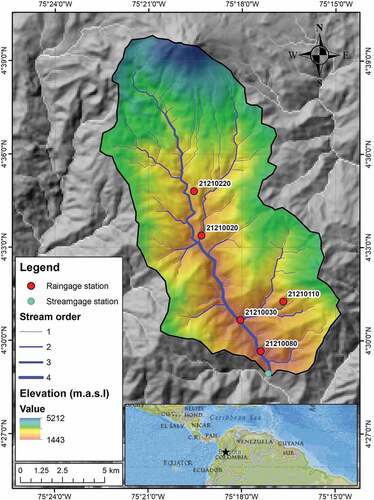
The current study was carried out in the Combeima River basin, whose headwaters are fed by snowmelt from the Nevado del Tolima volcano that flows into the Coello River after a distance of 57.5 km. Its source is located at coordinates 4.664°N, -75.348°E and at an altitude of 5225 m a.s.l. Its mouth is at 4.322°N, -75.348°E and 68 m a.s.l. It is located in the northwestern part of the municipality of Ibagué on the eastern flank of the Central Cordillera (mountain range). It has an extension of 27 421 ha, draining an area equivalent to 18.2% of the municipality of Ibagué with an average channel slope of 7.8%. The basin is part of the protected area Parque Natural Nacional los Nevados (PNNN). Its buffer zone corresponds to 26.19% of the total area of the basin. For the development of this research, the closing point of the basin is the Montezuma limnigraphic station, given the existence of daily flow records. Therefore, the study area has an area of 18 404.21 ha, corresponding to 67.12% of the total area of the basin (Fig. 1).

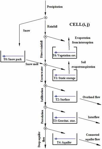
Figure 1. Cell conceptual scheme of the TETIS model (Francés et al. 2007).

There are five pluviographic stations in the basin that meet the World Meteorological Organization (WMO) criteria for hydrological modelling (Table 1). About 73% of the terrain has very steep to very undulating slopes, a factor that, together with the characteristics of its soils, makes mass movement phenomena the main threat issues of concern for the population and their productive activities. Regarding climatic aspects, the average annual temperature is 14°C, where the maximum and minimum registered are 24°C and −4°C. The annual potential evapotranspiration is 843 mm. The rainfall regime that characterizes the basin is bimodal, corresponding to two dry and two rainy seasons. The dry seasons occur in December–March and July–August, and the rainy seasons in April–June and September–November, with an average annual and average daily precipitation of 1816 mm and 4.2 mm, respectively. The average flow is 5.0 m³/s, and the maximum registered flows vary between 10.0 and 77.0 m³/s.

Table 1. Pluviographic stations selected in the study area.

					Coordinates N W
Pluviographic station	Name of pluviographic station	Elevation (m a.s.l.)	Municipality	Installation date (D/M/Y)	N (degrees)	W (degrees)
21 210 020	Juntas	1765	Ibagué	15 August 1971	4.5563	75.3216
21 210 030	Pastales	1505	Ibagué	15 May 1958	4.5111	75.3008
21 210 080	Secreto	1490	Ibagué	15 May 1985	4.4945	75.2901
21 210 110	Placer	2170	Ibagué	15 June 1983	4.5209	75.2779
21 210 220	Palmar	2200	Ibagué	15 August 1971	4.5801	75.3257

2.2 Hydrological model

The TETIS distributed hydrological model (Francés et al. 2007) was selected to consider an explicit representation of spatial variability. In order to discretize the basin at an appropriate level of detail, TETIS implemented a scale model whereby the effects of spatial variability and scale on the hydrological response will vary very little. For this reason the basin is sub-divided into rectangular elements (square cells) based on the digital elevation model (DEM). The drainage network is represented through the connection structure based on the flow direction scheme D8. Each cell delivers the flow only to a neighboring receiving cell in the direction of the steepest slope. In this way, runoff production is based on the realization of a water balance in each model cell.

The DEM is used to extract main geomorphological and morphological basin characteristics using geographic information systems tools, which combined with historical river gauge measurements are used to estimate the geomorphological kinematic wave parameters required by flow routing in the model.

In the TETIS model, the water is distributed in five levels or conceptual storage tanks that are interconnected. The flow between the tanks is a function of the water stored in them, so the state variables are the volumes stored in each tank. The function that relates the flow to these state variables is a function of the conceptual scheme adopted, the type of tank, and the morphological characteristics of the cell and hydrological characteristics of the soil and soil substrate. The TETIS hydrological model, among other aspects, considers the interception capacity of the vegetation cover, soil storage capacity, interflow, aquifer storage, and baseflow (Fig. 2). TETIS consider nine correction factors used as multipliers of the model parameter maps (Table 2); these factors are obtained in the calibration process of the model. The information used to develop the hydrological modelling process is described below.

Table 2. Parameters.

Correction factor ($R_i$)	Parameter ${\theta }_{i,j}^{\ast }$	Symbol	Range	Calibration values
FC1	Static storage capacity	$H_u$	[0.5–2.0]	0.5053
FC2	Plant cover index		[0.5–1.5]	0.5
FC3	Infiltration capacity	$K_s$	[0.001–10.0]	0.257
FC4	Surface flow velocity	$U$	[0.001–10.0]	1.5
FC5	Percolation capacity	$K_p$	[0.001–10.0]	0.0021
FC6	Interflow velocity	$K_{ss}$	[1.0–1000.0]	1.1641
FC7	Deep percolation capacity	$K_{ps}$	[0.0–0.1]	9.0834
FC8	Baseflow velocity	$K_{sa}$	[1–100.0]	0.6366
FC9	Flow velocity in the channel	$V$	[0.5–1.5]	1

Figure 2. Location of the study area.

2.2.1 Historical hydrometeorological information

The hydrological simulation was carried out daily using the Nash-Sutcliffe index as a metric to quantify the error between the observed and simulated flow. The 2006–2008 period was selected for model calibration and the 2003–2004 period for validation at the Montezuma hydrometric station.

2.2.2 Thematic cartographic information

The estimation of the parameters that control the flow and storage thresholds in the hydrological model was carried out by obtaining reference modal values based on the following cartographic information:

• Land cover and use maps at scales of 1:100 000 and 1:25 000 elaborated for the department of Tolima by Corporación Autónoma Regional del Tolima (CORTOLIMA, 2007).

• General study of soils and land zoning for the department of Tolima at a scale of 1:100 000 prepared by Instituto Geográfico Agustín Codazzi of Colombia (IGAC 2008).

• Surface geology map prepared by Geotec at a scale of 1:100 000 (Geotec 2012).

• Shuttle Radar Topography Mission (SRTM) digital elevation model at 90 m resolution, elaborated by the National Aeronautics and Space Administration of the United States of America (NASA , 2005).

• Information on hydraulic connections, i.e. the water uptake system for human consumption from the Combeima River in an upstream point of the model calibration station.

The scarce information available that represents the spatial heterogeneity in the modelled basin required the use of indirect methods to estimate the hydraulic properties of the soil and its substrate through pedotransfer functions, as described below.

2.2.3 Static storage (Hu)

The static storage (Hu) was calculated employing the general soil study information of IGAC (2008), indirectly through the pedotransfer functions of Saxton and Rawls (2006). Hu is expressed in mm and was estimated using Equation (1)(1) $Hu=\frac{\rho b\ast pAW}{\rho w\ast 100}+As+Imax$(1) :

(1) $Hu=\frac{\rho b\ast pAW}{\rho w\ast 100}+As+Imax$(1)

Hu represents the available water content in the soil plus surface storage (mm), ρb is the apparent density of the soil profile (g/cm³), ρw is the water density (g/cm³), and p corresponds to the minimum value between the soil thickness and the effective root depth (m). Further, AW is the water available for plants in the soil profile (%), and As is the surface water storage (mm) retained due to the effect of terrain roughness, essentially affected by the cover and the topographic slope. Finally, Imax represents the maximum interception capacity of the vegetation cover canopy.

2.2.4 Saturated hydraulic conductivity (Ks)

The saturated hydraulic conductivity (Ks) is calculated as the weighted value for each horizontal soil layer according to the depth of each of the profiles that compose it. It corresponds to the gravitational infiltration capacity and is defined as the capacity of porous media in saturated conditions to transmit water from one point to another (Montoya 2008). It is related to the type of soil and its structure. In TETIS, it is responsible for the passage of gravitational water and is associated with the type of soil and cover. In this case, Ks corresponds to the vertical saturated hydraulic conductivity, and Kss is the horizontal, which is usually higher (Wong et al. 2009). Equation (2)(2) $Kss=1/{\sum }_i^{n}1/K{s}_i\ast Pr{h}_i/Prp$(2) was used to calculate the Kss parameter:

(2) $Kss=1/{\sum }_i^{n}1/K{s}_i\ast Pr{h}_i/Prp$(2)

$K{s}_i$ is the vertical saturated hydraulic conductivity of the ith horizon of the soil profile (mm/h), $Pr{h}_i$ is the depth of the ith horizon of the soil profile (m), and $Prp$ is the total depth of the soil profile (m).

2.2.5 Percolation capacity (Kp)

The percolation capacity (Kp) was calculated using the methodology proposed by Chilton (1996) and estimating these values in metres per day. This value was then converted to millimetres per hour for the rocky substrate percolation capacity.

2.2.6 Interception capacity (Imax)

The interception capacity (Imax) corresponds to the land cover’s capacity to retain precipitation water. Its magnitude is determined by the cover type and its stratification in height for each model cell. The values adopted for this parameter are expressed in mm and are presented in Table 3.

Table 3. Plant cover indices and interception capacity.

Plant cover	J	F	M	A	M	J	J	A	S	O	N	D	Interception capacity (mm)
Forests	0.6	0.75	0.85	1	1	1	1	1	1	0.85	0.75	0.6	9
Crops	0.3	0.35	0.5	0.6	0.77	0.9	0.98	1	1	0.98	0.9	0.78	1
Pastures	0.48	0.6	0.75	0.85	0.87	0.9	0.9	0.87	0.85	0.8	0.65	0.6	1
Rocks, bare soil	1	1	1	1	1	1	1	1	1	1	1	1	0

2.2.7 Vegetation cover index (${\lambda }_m$)

The vegetation cover index (${\lambda }_m$) considers coverage indices that describe this dynamic during the annual cycle in a monthly resolution (m) due to the spatial and temporal variation of evapotranspiration. In this case, a reclassification of the land cover was carried out, grouping cover types such as forests, crops, pastures, and impervious areas, thus defining the values of the coverage index and the reclassified interception capacity, as presented in Table 3. These values were adopted from those reported in the literature (Allen et al. 1998, Allen 2000, Daza et al. 2009, Liu and Luo 2010, Steduto et al. 2012, Cuo et al. 2013). Therefore, considering the FAO (1998) reference values and the leaf area index, the seasonal variation coefficients of evapotranspiration were defined.

Flow propagation in channels in the TETIS hydrological model is carried out using the concept of a geomorphological kinematic wave (Francés et al. 2007). It establishes nine geomorphological parameters related through potential expressions whose coefficients (propagation parameters) adopted for the study case are presented in Table 4.

Table 4. Geomorphological propagation parameters adopted.

Propagation parameters	Range	Adopted
Coefficient ($K$)	0.5–0.75	0.6
Exponent ($\phi$)	0.65–0.8	0.75
Coefficient ($C_1$)	0.5–5.75	3.26
Exponent (${\alpha }_1$)	0.34–0.55	0.5
Exponent (${\alpha }_2$)	0.05–0.2	0.2
Coefficient ($C_d$)	0.5–50	20
Exponent ($\theta$)	0.5–2.75	1
Coefficient ($C_n$)	0.025–0.07	0.047
Exponent ($\xi$)	0.125–0.18	0.1667

Source: Francés et al. (2007).

The automatic calibration method of the TETIS model involves a structuring of parameters based on correction factors. These factors absorb errors from all the sources mentioned above. It is reasonable to assume that the correction factor is common for all basin areas, or at least for a limited number of regions within the basin. Furthermore, since all the cells have the same size, the scale effects are the same for the entire basin. Table 2 presents these factors, including the value obtained for each of them in the calibration process.

The main advantage of this parameter structure is that, in the calibration phase, the number of variables that must be adjusted is notably reduced, being necessary only to calibrate the p correction factors instead of the np values (number of parameters per number of cells).

2.3 The error model and uncertainty estimation

Data that show high values of asymmetry and kurtosis are poorly represented by the most common probability distribution functions, as is the case for daily precipitation, so it is necessary to use distributions that can model these characteristics. Along these lines, Azzalini (1985) studied the SN distribution to analyse data with an asymmetry and kurtosis coefficient outside the range allowed by a normal distribution, concluding that the phenomenon of asymmetry in the distribution is appropriately represented in the distribution of errors. This probability density function is given by Equation (3):

(3) $f\left(z\right)={\phi }_n\left(z,\mu ,\mathrm{\Omega }\right)\frac{\mathrm{\Phi }({\alpha }_0+{\lambda }^t\left(z-\mu \right)}{\mathrm{\Phi }\left(\tau \right)}$(3)

where ${\alpha }_0$ is a function of $\left(\mathrm{\Omega },\lambda ,\tau \right)$;

${\phi }_n\left(z,\mu ,\mathrm{\Omega }\right)$ is the n-dimensional normal density;

$\mathrm{\Phi }\left(.\right)$ is the standard distribution function $N\left(0,1\right)$; and

λ is an n-dimensional vector called the skew parameter.

When τ = 0, α₀ = 0. Equation (3)(3) $f\left(z\right)={\phi }_n\left(z,\mu ,\mathrm{\Omega }\right)\frac{\mathrm{\Phi }({\alpha }_0+{\lambda }^t\left(z-\mu \right)}{\mathrm{\Phi }\left(\tau \right)}$(3) is reduced to the multivariate SN distribution studied by Azzalini and Dalla Valle (1996), given by Equation (4):

(4) $f\left(Z\right)=2\mathrm{\varnothing }\left(Z;\mu ;\mathrm{\Omega }\right)\varphi \left(({\lambda }^t\left(Z-\mu \right)\right)$(4)

where λ regulates the distributional form. When λ = 0, the situation returns to normal. The density (Equation 3(3) $f\left(z\right)={\phi }_n\left(z,\mu ,\mathrm{\Omega }\right)\frac{\mathrm{\Phi }({\alpha }_0+{\lambda }^t\left(z-\mu \right)}{\mathrm{\Phi }\left(\tau \right)}$(3) ) comes from Azzalini and Capitanio (1999).

To derive the error model, with which the uncertainty of the precipitation variable is studied, Castro (2008) used the probabilistic reduction approach, for which he considered the marginal-conditional decomposition of the joint density and studied the relationship between the associated parameter spaces and the marginal and conditional models.

The study of the uncertainty of the precipitation variable was carried out through the quantification of the error model. For this quantification a mixed linear normal skew model of random effects was applied, as proposed by Arellano-Valle (2005), Rodrigues (2006) and Kheradmandi and Rasekh (2005) using conditional simulation. These models are the most common statistical tools for analysing agricultural and environmental data. Interest has been focused on the study of the estimation of parameters in measurement error models. Clark et al. (2008) state that this method can provide a better description of rainfall errors (Equation 5(5) $\begin{array}{c}{y}_i={\beta }_0+{\beta }_1{x}_i+\delta w+{\epsilon }_i\\ \hat{\mu }=\widehat{{\beta }_0}+\widehat{{\beta }_1}{\chi }_i+\hat{\delta }w\\ {\hat{y}}_i=E\left(y_i\right)=\hat{\beta }0+\hat{\beta }1x_i+\hat{\delta }w\end{array}$(5) ), as follows:

(5) $\begin{array}{c}{y}_i={\beta }_0+{\beta }_1{x}_i+\delta w+{\epsilon }_i\\ \hat{\mu }=\widehat{{\beta }_0}+\widehat{{\beta }_1}{\chi }_i+\hat{\delta }w\\ {\hat{y}}_i=E\left(y_i\right)=\hat{\beta }0+\hat{\beta }1x_i+\hat{\delta }w\end{array}$(5)

where yi is rainfall; xi is discharge; β₀ and β1 are fixed parameters; δ is a random-effects parameter; and w is the error of the independent variable. ${\epsilon }_i={\sum }_{i=1}^n{\left(Y_{iobserved}-Y_i\right)}^2$. It is assumed that ε_{i ~} SN (0, δ²_e, λ_x), and x_{i ~} SN (0, δ²_x, λ_x); the parameters of the distribution SN are 0 location, δ²e_x scale, and λ_x shape. The above equation represents the stochastic model of rainfall conditioned to observed discharge by assuming an SN distribution of rainfall error.

To consider a structural SN mixed measurement error model, under the model defined by Equation (5)(5) $\begin{array}{c}{y}_i={\beta }_0+{\beta }_1{x}_i+\delta w+{\epsilon }_i\\ \hat{\mu }=\widehat{{\beta }_0}+\widehat{{\beta }_1}{\chi }_i+\hat{\delta }w\\ {\hat{y}}_i=E\left(y_i\right)=\hat{\beta }0+\hat{\beta }1x_i+\hat{\delta }w\end{array}$(5) , we assume that:

(6) $\begin{array}{c}{\epsilon }_i\sim SN\left(0,{\sigma }^2,\lambda \right)x_i\sim SN\left(0,{\sigma }_x^2,{\lambda }_x\right)\\ {\delta }_i\sim SN\left(0,{\sigma }_b^2,{\lambda }_b\right)\end{array}$(6)

where (x, ε, δ) are independent. Leading, under the above model, we have:

(7) $y_i|x_i,{\delta }_i\sim \mathrm{S}\mathrm{N}({\beta }_0+{\beta }_{1}xi+\delta \mathrm{w},{\sigma }_e^2,{\lambda }_e)$(7)

3 Results

The TETIS hydrological model was calibrated by adjusting nine correction factors (Table 4). An automatic calibration procedure was carried out in the model using the shuffled complex evolution (SCE-UA) optimization algorithm implemented in the TETIS model by Vélez (2003). Calibration was performed daily, taking the values simulated over a warm-up period of one year as initial humidity conditions.

The Nash-Sutcliffe index value obtained for the calibration period was 0.61, while a value of 0.56 was registered for the validation. Thus, the model acceptably reproduces the flows in the basin since, according to the literature, a Nash-Sutcliffe index higher than 0.5 is considered acceptable.

The proposed error model (yi = β0 + β1xi + δw + εi) was initially solved through a Bayesian approach to calculate the uncertainty of each of the pluviometric stations. This approach used the WINBUSG software, for which two chains, a sample of 100 000 iterations implemented through the Gibbs sampling algorithm, and a warm-up time (burn-in) of 4000 iterations were used. This was done to discard the first m samples, given that there may be a strong correlation between sample realizations. The precipitation data used included 4383 observations, corresponding to a series from 1998 to 2009.

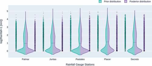
The SN distribution function showed a satisfactory fit to the observed rain data in the five evaluated pluviometric stations. As can be seen in Fig. 3, the a posteriori distribution function manages to reproduce the shape and statistics of the empirical distribution of the observed rainfall data at all stations (Table 5).

Table 5. Summary statistics estimated through Bayesian inference for each rainfall dataset.

Estación	Node	Mean	SD	MC error	2.50%	Median	97.50%
Palmar	β0	−0.10	0.01	0.00	−0.12	−0.09	−0.08
	β1	0.00	0.64	0.04	−0.12	0.00	0.00
	δ	7.78	0.04	0.00	7.68	7.78	7.86
	tau	1234.00	278.00	12.91	765.50	1212.00	1831.00
	tau1	0.00	0.20	0.01	0.00	0.83	0.00
Juntas	β0	−0.09	0.01	0.52	−121.00	−9036.00	−6729.00
	β1	−0.89	0.96	0.04	0.00	−0.65	0.42
	δ	8.92	0.13	0.01	8.72	8.87	9.13
	tau	1083.00	274.60	9.16	625.60	1055.00	1696.00
	tau1	0.99	0.26	0.00	0.59	0.00	0.00
Pastales	β0	−0.11	0.02	0.79	−0.15	−0.11	−0.08
	β1	−0.69	0.99	0.04	0.00	−0.87	0.92
	δ	11.90	0.22	0.01	11.54	12.00	12.17
	tau	890.90	256.10	9.68	467.50	862.30	1474.00
	tau1	0.00	0.37	0.01	0.68	0.00	0.00
Placer	β0	−0.11	0.02	0.00	−0.16	−0.11	−0.08
	β1	−0.39	0.68	0.04	0.00	−0.12	0.49
	δ	12.77	0.05	0.00	12.66	12.78	12.86
	tau	854.70	248.00	13.51	447.70	834.20	1383.00
	tau1	0.00	0.40	0.02	0.72	0.00	0.00
Secreto	β0	−0.11	0.02	0.00	−0.15	−0.11	−0.08
	β1	0.04	0.71	0.06	0.00	0.12	0.00
	δ	12.38	0.10	0.01	12.23	12.45	12.50
	tau	837.10	197.90	15.44	531.10	818.20	1307.00
	tau1	0.00	0.29	0.00	0.77	0.00	0.00

SD: Standard deviation, MC error: computational accuracy of the mean error.

Figure 3. Violin plots reporting the prior and posterior distributions of rainfall by applying the error algorithm based on a skew normal distribution for each rainfall dataset.

The propagation of precipitation uncertainty to discharge simulations was analysed through the definition of eight scenarios of rainfall input in the model. The scenarios were based on the number and location of the pluviometric stations in the watershed; by combining these into groups of five stations (one group), four stations (three groups), and three stations (four groups), the observed precipitation for each of the selected stations of the Combeima River Basin was corrected with the estimated uncertainty values based on the fitted SN distribution. In this way, discharge was simulated with the TETIS distributed hydrological model, obtaining the confidence bands for the simulated flow. Likewise, the flow of the Combeima River was simulated for eight scenarios.

Figure 4 shows the simulated flows for the TETIS hydrological model, with the average rainfall realizations corresponding to the blue line. Likewise, when executing the flow simulation the rain corresponds to the upper band (97.5%) of the error model and the lower band (2.5%), whose area is represented in the grey region.

Figure 4. Confidence band for the simulated flow in the Combeima River basin in eight combination scenarios of precipitation series. (a) Scenario with the stations Palmar, Juntas, and Placer; (b) scenario with the stations Palmar, Juntas, and Pastales; (c) scenario with the stations Palmar, Juntas, and Secreto; (d) scenario with the stations Placer, Pastales, and Juntas; (e) scenario with the stations Palmar, Juntas, Placer, and Secreto; (f) scenario with the stations Palmar, Juntas, Pastales, and Secreto; (g) scenario with the stations Juntas, Placer, Pastales, and Secreto; (h) scenario with the stations Palmar, Juntas, Placer, Pastales, and Secreto.

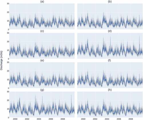
In order to analyse the effect of the propagation of rainfall uncertainty on the flow rate with respect to the spatial distribution of the rainfall stations, eight scenarios were proposed; each scenario was processed with a different number of rainfall stations, so that scenario a uses three stations, while scenario h was processed with the total number of stations.

There is a big difference in model efficiency when it is processed with scenarios a, b, c, e, f, and h that incorporate the precipitation series of the Palmar station, in contrast to the efficiency registered when scenarios d and g, which do not include this station’s data, are used (Table 5). Discharge model simulation is improved when precipitation data measured through this station is considered, and model performance is less sensitive to the number of rainfall gauge stations used in this case study. Therefore, simulation uncertainty is more sensitive to location than to the number of raingauge stations used to force the hydrological model in this poorly gauged basin.

The probability plot shows the best adjustments of flow simulations with observed discharge in the scenarios that include the El Palmar rainfall station (a, b, c, e, f and h), compared to scenarios d and g. Scenario b visualizes the best fit corresponding to the results of Table 6 and Fig. 5. The lowest bias in the simulated flows is obtained when using the El Palmar, El Secreto and Juntas rainfall stations (scenario b).

Table 6. Effect of rainfall scenario on model efficiency for the median simulated discharge vs. the observed discharge. Efficiency is expressed by the relative bias percentage (Bias) and Kling-Gupta efficiency (KGE).

	Scenario (a)	Scenario (b)	Scenario (c)	Scenario (d)	Scenario (e)	Scenario (f)	Scenario (g)	Scenario (h)
Bias (%)	5.5	2.2	3.0	24.5	10.5	8.0	28.4	13.3
KGE	0.58	0.58	0.61	0.48	0.59	0.59	0.46	0.57

Figure 5. Probability plot results of discharge simulation for the analysed scenarios regarding the number and distribution of the pluviometric stations. (A) Scenario with the stations Palmar, Juntas, and Placer; (B) scenario with the stations Palmar, Juntas, and Pastales; (C) scenario with the stations Palmar, Juntas, and Secreto; (D) scenario with the stations Placer, Pastales, and Juntas; (E) scenario with the stations Palmar, Juntas, Placer, and Secreto; (F) scenario with the stations Palmar, Juntas, Pastales, and Secreto;(G) scenario with the stations Juntas, Placer, Pastales, and Secreto; (H) scenario with the stations Palmar, Juntas, Placer, Pastales, and Secreto.

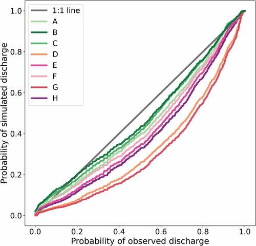
These results indicate how precipitation uncertainty significantly affects flow simulations for the Combeima River. Furthermore, the effect of the spatial distribution of the pluviometric stations is included since it was observed that flow estimation shows large differences when some stations are left out. This occurred when the calculations were carried out using the station scenarios but excluding one or two rainy stations from the simulation in each case.

4 Conclusions

Given the manifest importance of a sound quantitative understanding of data and model uncertainties in integrated water resources management, further development and implementation of instrumental and statistical procedures are needed to estimate hydrological data accurately and precisely. With its philosophy of using and refining knowledge of all uncertain quantities, the Bayesian paradigm provides a robust platform for systematically integrating this knowledge into hydrological model simulation and prediction.

As every modelling process simplifies reality, it is logical that its quantification shows important variations compared to reality, and differences can be studied and established through uncertainty, which, under a systemic approach, would be framed through one of its properties as entropy. Hence, it is very important to study this degree of ignorance of the system through uncertainty estimation.

The potential of using the error model in the context of Bayesian inference should be addressed as a tool for calculating the uncertainty in precipitation to capture its fundamental characteristics. This occurs because some methodologies, such as storm multipliers or the use of synthetic rains, do not allow reasearchers to infer these characteristics, only the effect of this uncertainty in the flow.

Acknowledgments

The authors acknowledge IDEAM, IGAC, and CORTOLIMA in Colombia for providing meteorological data, the soil study of the Tolima Region, and the land cover maps of the Tolima region. This work was partially supported by the doctoral fellowship programme of Universidad del Tolima [Agreement 146/15-09-2010] and the research project of Universidad del Tolima C050620.

Disclosure statement

No potential conflict of interest was reported by the author(s).

Additional information

Funding

This work was supported by the Universidad del Tolima [Agreement 146/15-09-2010, Project C050620].

References

- Allen, R.G., et al., 1998. Crop evapotranspiration: guidelines for computing crop requirements. Irrigation and Drainage Paper No. 56, FAO.
- Allen, R.G., 2000. Using the FAO-56 dual crop coefficient method over an irrigated region as part of an evapotranspiration intercomparison study. Journal of Hydrology, 229 (1–2), 27–41. doi:10.1016/S0022-1694(99)00194-8
- Andreassian, V., et al., 2001. Impact of imperfect rainfall knowledge on the efficiency and the parameters of watershed models. Journal of Hydrology, 250 (1–4), 206–223. doi:10.1016/S0022-1694(01)00437-1
- Arellano-Valle, R.B., Bolfarine, H., and Lachos, V.H., 2005. Skew-normal Linear Mixed Models. Journal of Data Science, 3, 415–438.
- Azzalini, A., 1985. A class of distributions, which includes the normal ones. Scandinavian Journal of Statistics, 12 (2), 171–178.
- Azzalini, A. and Capitanio, A., 1999. Statistical applications of the multivariate skew normal distribution. Journal of the Royal Statistical Society: Series B, 61 (3), 579–602. doi:10.1111/1467-9868.00194
- Azzalini, A. and Dalla Valle, A., 1996. The multivariate skew-normal distribution. Biometrika, 83 (4), 715–726. doi:10.1093/biomet/83.4.715
- Bárdossy, A. and Das, T., 2008. Influence of rainfall observation network on model calibration and application. Hydrology and Earth System Sciences, 12 (1), 77–89. doi:10.5194/hess-12-77-2008
- Biemans, H., et al., 2009. Effects of precipitation uncertainty on discharge calculations for main river basins. Journal of Hydrometeorology, 10 (4), 1011–1025. doi:10.1175/2008JHM1067.1
- Castro, L.M., 2008. Distribución Skewnormal: identificabilidad, Reducción y Enfoques Bayesianos de Mezclas. PhD Thesis. Universidad Católica de Chile.
- Chilton, J., 1996. Chapter 9 - groundwater, and D. Chapman, ed. Water quality assessments. A guide to use of biota, sediments and water in environmental monitoring. Vol. 5. London: E&FN Spon, 651.
- Clark, M.P., et al., 2008. Framework for understanding structural errors (FUSE): a modular framework to diagnose differences between hydrological models. Water Resources Research, 44 (12). doi:10.1029/2007WR006735
- CORTOLIMA, 2007. Land use and land cover study for department of Tolima. Colombia: Corporación Autónoma Regional del Tolima, Ibagué, Colombia.
- Cuo, L., et al., 2013. The impacts of climate change and land cover/use transition on the hydrology in the upper Yellow River Basin, China. Journal of Hydrology, 502, 37–52. doi:10.1016/j.jhydrol.2013.08.003
- Daza, M.C., Hernandez, F., and Triana, F.A., 2009. Efecto de actividades agropecuarias en la capacidad de infiltración de los suelos del páramo del sumapaz. Ingeniería de Recursos Naturales y del Ambiente, 8 (8), 29–39.
- FAO. (1998). Irrigation and drainage paper No. 56. Crop evapotranspiration (guidelines for computing crop water requirements). FAO.
- Fraga, I., Cea, L., and Puertas, J., 2019. Effect of rainfall uncertainty on the performance of physically based rainfall–runoff models. Hydrological Processes, 33 (1), 160–173. doi:10.1002/hyp.13319
- Francés, F., Vélez, J.I., and Vélez, J.J., 2007. Split-parameter structure for the automatic calibration of distributed hydrological models. Journal of Hydrology, 332 (1–2), 226–240. doi:10.1016/j.jhydrol.2006.06.032
- Geotec, 2012. Estudio de amenazas naturales, vulnerabilidad y escenarios de riesgo en los centros poblados de Villarestrepo, Llanitos, Juntas, Pastales, Pico de Oro, Bocatoma Combeima y Cay, por flujos torrenciales en las microcuencas del Río Combeima. Alcaldía de Ibagué, Cortolima. Ibagué, Colombia: Consorcio Geotec Group.
- Goetzinger, J. and Bárdossy, A., 2008. Generic error model for calibration and uncertainty estimation of hydrological models. Water Resources Research, 44, W00B07.
- Gupta, H.V., Beven, K., and Wagener, T., 2005. Model calibration and uncertainty estimation. In: M.G. Anderson and J.J. McDonnell, eds. Encyclopedia of hydrological sciences. Chichester, Reino Unido: John Wiley & Sons.
- IGAC, 2008. Estudio general de suelos y zonificación de tierras del departamento del Tolima. Instituto Geográfico Agustín Codazzi. Bogotá, Colombia: IGAC.
- Kavetski, D., Franks, S., and Kuczera, G., 2003. Confronting input uncertainty in environmental modelling. In: Q. Duan, et al., eds. Calibration of watershed models. Water Science and Applications Series. Washington D.C.: AGU, 49–68.
- Kavetski, D., Kuczera, G., and Franks, S.W., 2006a. Bayesian analysis of input uncertainty in hydrological modeling: 1. Theory. Water Resources Research, 42 (3), W03407.
- Kavetski, D., Kuczera, G., and Franks, S.W., 2006b. Bayesian analysis of input uncertainty in hydrological modeling: 2. Application. Water Resources Research, 42 (3), W03408.
- Kheradmandi, A., and Rasekh, A., 2005. Estimation in skew-normal linear mixed measurement error models. Journal of Multivariate Analysis, 136, 1–11.
- Liu, Y. and Gupta, H.V., 2007. Uncertainty in hydrologic modeling: toward an integrated data assimilation framework. Water Resources Research, 43 (7), 1–18. doi:10.1029/2006WR005756
- Liu, Y. and Luo, Y., 2010. A consolidated evaluation of the FAO-56 dual crop coefficient approach using the lysimeter data in the North China Plain. Agricultural Water Management, 97 (1), 31–40. doi:10.1016/j.agwat.2009.07.003
- Montanari, A. and Grossi, G., 2008. Estimating the uncertainty of hydrological forecasts: a statistical approach. Water Resources Research, 44 (12), W00B08. doi:10.1029/2008WR006897
- Montoya, J.J., 2008. Desarrollo de un modelo conceptual de producción, transporte y depósito de sedimentos Tesis doctoral no publicada. Universitat Politècnica de València. doi:10.4995/Thesis/10251/8303
- Moradkhani, H., et al., 2006. Investigating the impact of remotely sensed precipitation and hydrologic model uncertainties on the ensemble streamflow forecasting. Geophysical Research Letters, 33 (12). doi:10.1029/2006GL026855
- Moradkhani, H., and Sorooshian, S., 2008. General Review of Rainfall-Runoff Modeling: Model Calibration, Data Assimilation, and Uncertainty Analysis. In: S. Sorooshian, K.-L. Hsu, E. Coppola, B. Tomassetti, M. Verdecchia, and G. Vischonti, eds. Hydrological Modelling and the Water Cycle: Coupling the Atmospheric and Hydrological Models. Vol. 63. Berlin Heidelberg: Springer.
- NASA, 2005. Shuttle radar topography mission: the mission to map the world, available from Jet Propulsion Laboratory, California Institute of Technology. Available from: http://www2.jpl.nasa.gov/srtm/spanish.htm
- Pappenberger, F., et al., 2005. Cascading model uncertainty from medium range weather forecasts (10 days) through a rainfall-runoff model to flood inundation predictions within the European Flood Forecasting System (EFFS). Hydrology and Earth System Sciences, 9 (4), 381–393. doi:10.5194/hess-9-381-2005
- Renard, B., et al., 2011. Toward a reliable decomposition of predictive uncertainty in hydrological modeling: characterizing rainfall errors using conditional simulation. Water Resources Research, 47 (11), W11516. doi:10.1029/2011WR010643
- Rodrigues, J., 2006. A Bayesian inference for the extended skew-normal measurement error model. Brazilian Journal of Probability and Statistics, 20, 179–190.
- Saxton, K.E. and Rawls, W.J., 2006. Soil water characteristic estimates by texture and organic matter for hydrologic solutions. Soil Science Society of America Journal, 70 (5), 1569–1578. doi:10.2136/sssaj2005.0117
- Steduto, P., et al, 2012. Crop yield response to water. Report 66. Rome.
- Vélez, J.J., 2003. Desarrollo de un modelo distribuido de predicción en tiempo real para eventos de crecidas. PhD Tesis. Universidad Politécnica de Valencia.
- Wong, L.S., Hashim, R., and Ali, F.H., 2009. A review on hydraulic conductivity and compressibility of peat. Journal of Applied Sciences, 9 (18), 3207–3218. doi:10.3923/jas.2009.3207.3218
- Younger, P.M., Freer, J.E., and Beven, K.J., 2009. Detecting the effects of spatial variability of rainfall on hydrological modelling within an uncertainty analysis framework. Hydrological Processes, 23 (14), 1988–2003. doi:10.1002/hyp.7341