Impact of local versus global datasets on hydrological responses in Mahanadi River basin in India

ABSTRACT

Global environmental changes are likely to have a large impact on water resources across the developing countries. However, most of these countries suffer from acute shortage of local data. New high-resolution global products are available, which can be integrated with large-scale hydrological models. Most of these global products, however, are rarely evaluated in developing regions. We propose a thorough evaluation of five new global products in Mahanadi River basin in India. We employ the variable infiltration capacity (VIC) model over the basin and perform model experiments to directly evaluate the impacts of the specific combinations of local and global datasets. Results suggest that the reference experiment, which uses all local datasets, most closely represents the observed discharge. However, some of the global datasets could be used as a viable alternative to local observations in this river basin and potentially in nearby basins where there is a lack of observations.

KEYWORDS:

• variable infiltration capacity (VIC)
• global datasets
• local datasets
• discharge

Editor A. Fiori; Associate Editor A. Agarwal

1 Introduction

Global environmental changes such as land cover and climate changes are likely to impact the water resources of a region (Sterling et al. 2013, Bosmans et al. 2017, Chen et al. 2020). For developing countries, such impacts are expected to be even larger (Jin et al. 2018). However, modelling hydrological responses in developing countries faces additional challenges due to acute shortage of local data and limited monitoring capabilities (Bierkens et al. 2015, Rodríguez et al. 2020). Shortages in data are due either to a decline in the in situ monitoring gauges (Connor 2016) or the data not being openly accessible for research (Beria et al. 2017). For example, Mujumdar (2015) has recently highlighted the difficulties faced by the Indian hydrological community, owing to the reluctance of the relevant governmental organizations to openly share required hydro-meteorological data and its metadata with the research bodies. This limits the ongoing research of analysing real-time hydro-meteorological processes, amidst the continuously changing climate and its impact on water resources.

Recent advances in land surface models (Van Den Hurk et al. 2011, Fisher and Koven 2020) have resulted in the need for and availability of new high-resolution global products (Wood et al. 2011). Despite their availability, most of these global products are still heavily evaluated in developed regions making use of their dense monitoring networks (Sungmin et al. 2017, Gilewski and Nawalany 2018, Tang et al. 2020, Gao et al. 2020). This can, however, pose potential reliability risks when utilizing such products in regions where evaluation has not been properly carried out. This stresses the need to integrate high-quality global datasets into the land surface or hydrological models for data-scarce regions of the world (Strömqvist et al. 2009, Liu et al. 2011, Mujumdar 2015, Zubieta et al. 2016, Beria et al. 2017).

In recent years, there have been enormous advances in the global availability of geophysical attribute data, such as soil, vegetation and fine-scale meteorological data (Bierkens et al. 2015, Clark et al. 2015) from the ever-expanding remote sensing activities, reanalysis products and other large datasets. Understanding the information content in the available data, especially for data-scarce regions in the world, and how the land models use this information to simulate hydrological responses, is crucial for advancing the hydrological benchmarking activities to improve process representations in land surface models (Clark et al. 2015).

Both satellite and global reanalysis datasets are widely used for hydrological applications especially in data-sparse regions (Collischonn et al. 2007, Voisin et al. 2008, Shah and Mishra 2014a, Essou et al. 2016, Mahto and Mishra 2019). The launching of new earth observatory missions and better sensors has led to improvement in the quality of precipitation estimates worldwide (Huffman et al. 2007, 2015, 2018). For instance, emergence of The Integrated Multi-satellite Retrievals for Global Precipitation Measurement (GPM) (IMERG) in 2014 have improved the hydrological applications of satellite-based precipitation (Gilewski and Nawalany 2018). Recent studies have noted improvement in the precipitation quality of different versions of GPM IMERG over other satellite rainfall products such as the Tropical Rainfall Measuring Mission (TRMM) Multi-satellite, TRMM and Multi-satellite Precipitation Analysis (TMPA-3B42), TMPA V7, and others; in India and elsewhere (Prakash et al. 2018, Sharifi et al. 2016, Zubieta et al. 2016, Beria et al. 2017, Sungmin et al. 2017, Gilewski and Nawalany 2018, Tang et al. 2020). Simultaneously, the numerical weather prediction systems are also continuously improving (Mahto and Mishra 2019). For instance, Mahto and Mishra (2019) evaluated five new reanalysis products against local observations for hydrological applications in India. Analysis showed the European Centre for Medium-Range Weather Forecasts Reanalysis v5 (ERA5) captured the best monsoon season rainfall and maximum temperature compared with other reanalysis products such as Modern-Era Retrospective analysis for Research and Applications, Version 2 (MERRA-2), ERA-Interim, Climate Forecast System Reanalysis (CFSR), and the Japanese 55-year Reanalysis (JRA55). A recent development in the European Centre for Medium-Range Weather Forecasts (ECMWF) is the release of a global dataset for land component of ERA5, hereafter referred to as ERA5-Land (Muñoz-Sabater et al. 2021). In a recent study by Gao et al. (2020), ERA5-Land performed better than other reanalysis products while being outperformed by GPM IMERG for hydrological applications in China. The abilities of reanalysis datasets in hydrological predictions are less well explored compared to those of satellite datasets (Essou et al. 2016).

Global soil and land cover information is also available on a much finer spatial scale. Among the current global soil maps, the latest version of SoilGrids at a resolution of 250 m (Hengl et al. 2017) involves the most detailed estimation of soil distribution with the highest accuracy and resolution (Dai et al. 2019). Very few studies exist that test the impact of using global soil data in a hydrological model (Dembélé et al. 2020, Krpec et al. 2020); as one example, Krpec et al. (2020) tested the impacts of using global soil from SoilGrids on hydrological responses. Recently released time series of a global land cover product from the European Space Agency Climate Change Initiative (ESA CCI) of relatively finer resolution is an advancement over other available global land cover products such as the International Geosphere–Biosphere Programme (IGBP), Global Land Cover 2009 (GlobCover 2009) (Jiang and Yu 2018). Therefore, it is essential to evaluate the advancements and updates of these datasets in terms of their suitability for hydroclimatic applications in regional-scale studies (Strömqvist et al. 2009, Liu et al. 2011, Mujumdar 2015, Zubieta et al. 2016, Beria et al. 2017).

In this study, we propose a thorough evaluation of five new global products in a large basin in India, using a semi-distributed hydrological or land surface model, variable infiltration capacity (VIC). The Mahanadi River Basin, located in the eastern part of India, drains an area of 141 589 km² and has undergone severe environmental (both climate and land cover) changes during the last few decades, resulting in serious impact to its river flows. In addition, unlike other basins in the country, the Mahanadi River basin contains a relatively dense network of hydrometeorological and basin property variables that can be used to evaluate these global products. With the above motivation, we intend to answer the following research questions: (1) How does the inclusion of global datasets in a regional-scale hydrological model impact model predictions in a sub-tropical climate? or, How reliable are global datasets in producing a comparable hydrological model performance when compared against local observations? and (2) How can the impacts of those different inputs propagate to different hydrological components simulated by the model? This study is driven by the hypothesis that using all local datasets will result in better model performance compared to introducing global datasets in the model. The objectives of this study are to (1) perform various model experiments combining forcings, soil, and land use datasets from local and global products for hydrological predictions; and (2) comprehensively analyse the model performance of each experiment and identify critical input datasets or combinations of input datasets that may have significant impacts on model performance. Overall, this analysis aims to discern the hydrological impacts caused by the changes in a model input (local or global) or a combination of model inputs (local and global) to provide a basis for relying on the global data in a hydrological or land surface model for future use.

Very few studies exist that explore various combinations of input datasets to achieve maximum gain in hydrological model performance. Some past research papers focussed on selecting a proper combination of model inputs prior to model calibration (Faramarzi et al. 2015, Tarawneh et al. 2016) rather than assessing the impacts of global datasets for hydrological applications in different regions. Hence, there is a notable gap in the literature associated with evaluating global datasets in data-scarce regions. New studies are therefore needed to assess the suitability of using these global datasets for hydrological applications in different regions, especially in data-scarce regions like those in India. Our study is also an advancement over the few published studies (Kneis et al. 2014, Prakash et al. 2018, Shah and Mishra 2014b, Ghodichore et al. 2018, Mahto and Mishra 2019) in this domain as we evaluate the recently released and finer resolution global datasets which, to our knowledge, have not been tested yet in Indian river basins for hydrological applications.

2 Research area

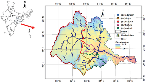
Mahanadi River basin is one of the major river basins of India, situated in the east-central part of the country (Fig. 1). The basin drains an area of 141 589 km², which accounts for nearly 4.3% of the total geographical area of India. The major percentage of the basin lies in the state of Orissa and Chhattisgarh, and the rest lies in Jharkhand, Maharashtra and Madhya Pradesh. The area of lowest elevation (−17 m) lies in the coastal reaches and the area of highest elevation (1323 m) is in the northern hills. Forest and agricultural lands are the dominant land uses in the basin. The basin has a tropical climate zone and receives rainfall from southwest monsoons during June–September. The average annual rainfall is 1572 mm, of which 80% is contributed in the monsoon season. The distribution of rainfall is uneven, resulting in floods in some parts of the basin and drought in others. The mean annual discharge is 1895 m³/s. The maximum temperature within the basin ranges from 39 to 45°C and the minimum temperature varies from 4 to 12°C. Clay and loam are the main soil textures in the basin. The basin consists of many dams, barrages and irrigation networks, among which Hirakud dam, with a gross storage capacity of 8136 km³, is the major hydro project in the basin. About 65% of the basin is located upstream of the dam (see Fig. 1). A dense network of raingauges consisting of 7000 stations is well spread across India, among which 201 raingauges exists within this basin.

Figure 1. The Mahanadi River basin boundary and the analysed gauges and their catchments. Abbreviations for gauge names are Ba, Basantpur; Ka, Kantamal; Ke, Kesinga; Su, Sundergarh; and Sa, Salebhata.

3 Materials and methods

3.1 VIC model

The VIC model is a grid-based semi-distributed, hydrological model that solves both water and energy balance at the land surface (Cherkauer and Lettenmaier 1999). The unique features of the VIC-3 L model include representing sub-grid heterogeneity in vegetation, multiple soil layers with variable infiltration rates and nonlinear baseflow. Generally three layers of soil are considered, where the top two soil layers represent the dynamic response to variable infiltration rates of incoming rainfall while the third soil layer characterizes baseflow processes (Yanto et al. 2017). A variable infiltration curve (Zhao et al. 1980) is used to generate the grid-based runoff within the model. Evapotranspiration occurs from all three soil layers in VIC. More descriptions regarding the VIC structure and formulations of model processes can be found in Liang et al. (1994). To obtain river discharge at the basin outlet, the VIC-3 L model is coupled to a stand-alone routing model (Lohmann et al. 1996).

We applied the VIC model version VIC 4.2.d using the water balance mode at a daily time step and 0.05° spatial resolution over the five sub-catchments of the Mahanadi River basin. We used the standard approach of using three root zones. Flows are routed to the sub-catchments of Basantpur (Ba), Kantamal (Ka), Kesinga (Ke), Sundergarh (Su) and Salebhata (Sa) (Fig. 1). We abstained from routing the flow for the entire Mahanadi River basin due to the presence of a major water management structure, Hirakud dam, in the middle reach of the basin.

3.2 Input datasets and parameters

The inputs required by VIC model are meteorological forcing (precipitation, maximum and minimum temperature, and wind speed), soil properties, land use and vegetation properties, and topographical details. The Cartosat-1 Digital Elevation Model (CartoDEM) 30, a national DEM developed by the Indian Space Research Organization (ISRO), is used for extracting all topographical features and for delineating the Mahanadi River basin. Sivasena Reddy and Janga Reddy (2015) evaluated six DEMs of different resolutions including the Shuttle Radar Topography Mission (SRTM) 90, CARTO 30 and the Advanced Spaceborne Thermal Emission and Reflection Radiometer (ASTER) 30, in an Indian river basin and found that CARTO 30 provided more accurate estimates of runoff and watershed areas than other DEMs. Therefore, we refrained from testing any global DEM in this study. Table 1 provides a summary of the input data used in this study.

Table 1. Summary of model input datasets used in this study.

Inputs	Resolution	Data availability/region
Land use
NRSC	50 m	Local
ESA CCI	300 m	Global
Soils
NBSS LUP	500 m	Local
SOIL GRIDS	250 m	Global
Precipitation
IMD	0.25° × 0.25°	Local
GPM IMERG	0.1° × 0.1°	Global
ERA5-Land	0.1° × 0.1°	Global
Temperature
IMD	1° × 1°	Local
ERA5-Land	0.1° × 0.1°	Global

3.2.1 Soil and Land Use Land Cover (LULC)

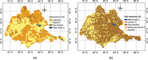
A national-level soil map is derived from the digitized soil map provided by the National Bureau of Soil Survey and Land Use Planning (NBBSSLUP) at a scale of 1:250 000 (Fig. 2(a)). Loam and clay are the dominant soil textures within the basin. Global gridded soil textures are derived from SoilGrids. The soil texture fractions of clay, sand and silt in SoilGrids are mapped at seven standard depths ranging from 0 to 200 cm. In this study, soil fraction maps of 30, 60, 100 and 200 cm (typical VIC soil depths) are averaged and resampled to a model grid size of 5 km. Next, fractions of clay, sand, and silt are extracted for each grid and the United States Department of Agriculture (USDA) soil classification is used to generate mean soil texture for each grid. For the sake of clarity, a global soil map for the basin (Fig. 2(b)) is shown at a model grid resolution of 5 km (instead of showing three different soil texture maps for clay, sand and silt at 250 m resolution). As per the global soil map, clay loam and clay are the dominant soil types in the river basin. We observe differences in the soil textures, and also the fractional area covered by each soil type, while comparing the two soil maps. The local soil map indicates loam (54%) and clay (42%) are the dominant soil textures within the basin, whereas clay (29%) and clay loam (69%) are found to be dominant in the global soil map.

Figure 2. (a) National soil map derived from the National Bureau of Soil Survey and Land Use Planning (NBBSSLUP) with a spatial resolution of 500 m; and (b) global soil map derived from SoilGrids with a spatial resolution of 250 m for the Mahanadi River basin. The spatial resolution of the maps shown here is 5 km, which is used by the VIC model to perform the simulations.

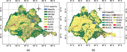
A national-level Land Use Land Cover (LULC) map is derived from the National Remote Sensing centre (NRSC) for the years 2013–2014 at a scale of 1:250 000 (Fig. 3(a)). A global LULC map for the year 2014 is obtained from the consistent series of annually generated land cover products from ESA CCI (version 2.0.7) (Jiang and Yu 2018) for the period 1992–2015 at a resolution of 300 m (Fig. 3(b)). Both the local and global LULC maps are reformatted and reclassified into United States Geological Survey (USGS) LULC types as required by the VIC model. Both LULC maps show that deciduous broadleaf forest (DBF) and cropland (CL) are the major land cover types in the basin. However, we observe that the percentages of area covered by these land cover types vary between the maps – especially CL, which covers 64% of the areaon the global map and 48% on the local map.

Figure 3. (a) National LULC map derived from National Remote Sensing centre (NRSC), India, for 2013–2014, with a resolution of 56 m; and (b) global LULC map derived from ESA CCI for 2014, with a resolution of 250 m.

The VIC model has 46 tuneable parameters (Bennett et al. 2018). We performed a global sensitivity analysis (GSA) on some soil, vegetation and routing parameters based on suggestions by VIC model developers (Gao et al. 2010) and the existing literature (Demaria et al. 2007, Yanto et al. 2017, Joseph et al. 2018, Gou et al. 2020). Among those parameters, the soil parameters infiltration capacity (binf), fraction of maximum velocity of baseflow (ds), velocity of baseflow (dsmax), soil moisture in the third soil layer (ws), second (d2) and third (d3) soil layer depth, and routing parameters (vel) are found to be sensitive and hence are subjected to calibration. The rest of the soil properties such as soil porosity (P), field capacity (fc), wilting point (wp), saturated hydraulic conductivity (ksat), initial soil moisture, etc. are obtained based on average hydraulic properties of USDA soil textural classes (Cosby et al. 1984, Rawls et al. 1998, Reynolds et al. 2000). Among the vegetation parameters, monthly mean Leaf Area Index (LAI) values are derived from the daily LAI product for the period 2000–2015 from Moderate Resolution Imaging Spectroradiometer (MODIS) AQUA/TERRA. We derived root zone depths and estimated the fractions of roots in each zone following Zeng (2002). Other related biophysical parameters required by VIC such as roughness, length, albedo, displacement height, etc., are assembled based on the Land Data Assimilation System (LDAS) (Naha et al. 2021).

3.2.2 Meteorological datasets

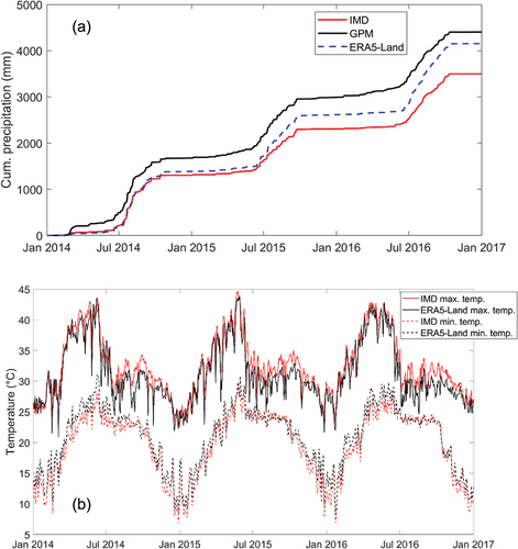
Precipitation datasets in this study are obtained from three sources: (1) daily gridded precipitation data from IMD at a grid resolution of 0.25° × 0.25°. For more details on the development of the IMD gridded dataset, refer to Pai et al. (2014); (2) half-hourly precipitation data from IMERG-VO6 with a spatial resolution of 0.1° × 0.1°. The IMERG algorithm uses all available sensors of TRMM and GPM eras to provide global precipitation estimates at a spatial resolution of 0.1° and a temporal resolution of 30 min. The latest version of this product, V06, is a retrospective processing of IMERG to the TRMM era and uses a new algorithm with several major improvements, which could enhance the quality of the precipitation estimates (Tang et al. 2020); (3) hourly precipitation data from ERA5-Land, the recently released new-era reanalysis product of ECMWF and a replay of the land component of ERA5 climate reanalysis with much finer spatial resolution of ~9 km compared to ERA5 (31 km) and ERA-Interim (80 km). As ERA5-Land is based on several improvements, most importantly the enhanced horizontal resolution (9 km vs 31 km) compared with ERA5, it is crucial to assess its suitability in hydrometeorological applications. Temperature data in this study is obtained from two sources: (1) daily gridded maximum and minimum temperature data from IMD at a resolution of 1° × 1°, developed using 395 stations and having 20 grids within Mahanadi River basin; (2) hourly temperature from ERA-Land with a horizontal resolution of ~9 km. The daily maximum and minimum temperature are derived from the hourly temperature. Wind speed is obtained from the National Center for Environmental Prediction (NCEP) and the National Center for Atmospheric Research (NCAR) reanalysis of resolution 1°. Note that both rainfall datasets from GPM and ERA5-Land and temperature from ERA5-Land were accumulated to the daily time scale, and the spatial resolutions of all datasets including IMD are kept at the VIC model resolution of 0.05°. Figure 4 shows cumulative daily precipitation and temperature at Basantpur from IMD, GPM IMERG and ERA5-Land, for the period 2014–2016. We performed quality comparisons of the precipitation and temperature products for the analysis period 2014–2016, prior to using these datasets as the model inputs to capture the hydrological responses. A comparison of the rainfall and temperature products from different sources is beneficial to understand their error characteristics and how error propagates to the estimated hydrological components. The Appendix shows a preliminary analysis of these comparisons.

Figure 4. (a) Cumulative daily precipitation of sub-basin Basantpur from IMD, GPM IMERG and ERA5-Land, for the period 2014–2016. (b) Daily minimum and maximum temperatures for sub-basin Basantpur from IMD and ERA5-Land, for the period 2014–2016.

3.3 Experimental design and model evaluation

Precipitation, temperature, soil, and land use datasets from local and global products are combined to yield 11 model experiments (Table 2). These experiments are designed with the objective of testing the impacts on model performance of using (1) all local datasets (exp1); (2) combinations of local and global datasets (exp2,3,4,5,6,7,8,9); and (3) all global datasets (exp10,11) in a hydrological model. Exp3 and exp4 use global precipitation datasets from GPM and ERA5-Land, respectively, while the rest of the inputs are local. Exp7 and exp8 are designed to test global soil and land cover, respectively. Exp9 is a follow-up to exp6 and exp7 where we test the hydrological response of using both soil and land cover from global sources. In exp2 we replace coarse-resolution local temperature from IMD with fine-resolution temperature from ERA5-Land. Exp5 and exp6 are framed to understand the impact of using both rainfall and temperature datasets from global products. Exp10 and exp11 are used to test the impact of using all global datasets as model inputs. The difference between exp10 and exp11 is the source of the global rainfall product, i.e. they use GPM and ERA5-Land, respectively.

Table 2. Description of the experiments performed in this study.

Experiments	Local	Global
1	IMD rainfall, IMD temperature, soil, LULC types	-
2	IMD rainfall, soil textures, LULC types	ERA5-Land temperature
3	IMD temperature, soil textures, LULC types	GPM rainfall
4	IMD temperature, soil textures, LULC types	ERA5-Land rainfall
5	Soil textures, LULC types	GPM rainfall, Reanalysis ERA5-Land temperature
6	Soil textures, LULC types	ERA5-Land rainfall, ERA5-Land temperature
7	IMD rainfall, IMD temperature, LULC types	Soil textures
8	IMD rainfall, IMD temperature, soil textures	LULC types
9	IMD rainfall, IMD temperature	Soil textures, LULC types
10	-	GPM rainfall, ERA5-Land temperature, soil, LULC
11	-	ERA5-Land rainfall, ERA5-Land temperature, soil, LULC

A set of behavioural models (250 models) are first obtained by calibrating the model using all local datasets, using a sequence of 5000 Monte Carlo simulations, for the time period 1990–2010 including a two-year warm-up period (1988–1999). We use Klein-Gupta efficiency (KGE) (Gupta et al. 2009) as an objective function to assess the model performance in the calibration period. Full details on the VIC model set-up and model calibration for the Mahanadi River basin can be found in Naha et al. (2021) and the supplemental section of this paper (https://doi.org/10.5194/hess-25-6339-2021-supplement).

Next, all experiments, including exp1 (experiment using all local datasets) are run using these behavioural models for an entirely different time period (2014–2016), owing to the availability of the datasets. These behavioural models consider uncertainties in the model outcome stemming from model parameterization or any biases in the input datasets. The VIC model in this study is set up to produce daily streamflow at all sub-catchments shown in Fig. 1. To ensure accurate initialization of the VIC soil moisture for the rest of the experiments (exp2–11), the behavioural models are spun up by forcing data of 2014–2016 repeatedly for 21 years (seven loops through a three-year period) following the recommendation of Rodell et al. (2005). Since we calibrated the models using local datasets, exp 1 is considered the reference or benchmark simulation. It is worth mentioning that we restrict our study to a shorter analysis period, i.e. only three years, due to the lack of availability of the local daily estimates of maximum and minimum IMD temperature beyond the year 2016. The observed discharge data at multiple gauges (Fig. 1) for the period 1988–2010 are available from the Central Water Commission (CWC), India.

The model performance was evaluated by quantitative comparison with the observed discharge using the KGE performance metric (Equations 1(1) $\mathrm{K}\mathrm{G}\mathrm{E}=1-\sqrt{{\left(\mathrm{r}-1\right)}^2+{(\alpha -1)}^2+{(\beta -1)}^2,}$(1) –3(3) $\beta =\frac{{\mu }_{sim}}{{\mu }_{obs}}$(3) ). KGE balances the contribution to the error coming from all three main components, namely correlation (e.g. timing/dynamics), variability (e.g. seasonality), and systematic bias, and is widely used in hydrometeorological studies (Gupta et al. 2009, Rodriguez and Tomasella 2016, Knoben et al. 2019, Tang et al. 2020, Mishra et al. 2020). The KGE range is [−∞,1] with values closer to 1 indicating better performance.

(1) $\mathrm{K}\mathrm{G}\mathrm{E}=1-\sqrt{{\left(\mathrm{r}-1\right)}^2+{(\alpha -1)}^2+{(\beta -1)}^2,}$(1)

(2) $\alpha =\frac{{\sigma }_{sim}}{{\sigma }_{obs}}$(2)

(3) $\beta =\frac{{\mu }_{sim}}{{\mu }_{obs}}$(3)

where r is the linear correlation between observed and simulated discharge, $\alpha$ is an estimate of flow variability error and $\beta$ is a bias term. ${\sigma }_{sim}$ and ${\sigma }_{obs}$ are the standard deviations of simulated and observed discharge, respectively. ${\mu }_{sim}$ and ${\mu }_{obs}$ are the mean of simulated and observed discharge, respectively.

4 Results

4.1 Model performance of all experiments

Calibration of the VIC model is performed against a local dataset on a daily time scale with respect to KGE for the period 1990–2000 for all the sub-catchments. Overall, the model reproduced the observed flows remarkably well, with median KGE values of 0.85, 0.86, 0.82, 0.75 and 0.63 at Basantpur, Kantamal, Kesinga, Salebhata and Sundergarh, respectively (see Fig. S1 in the Supplementary material). These calibrated models are then used in a completely different period (2014–2016) to evaluate the simulated daily discharge from the 11 VIC model experiments (Table 2) for the sub-catchments of the Mahanadi River basin. Figure 5 (top panel) shows the model performance (KGE) for the simulated discharge obtained from the 11 model experiments against the observed discharge for all sub-catchments. The box plots represent uncertainties in the KGE values due to different model parameterizations (or 250 behavioural models). We averaged the ranks achieved by each experiment at all sub-basins to obtain an overview of the model performances. The benchmark or reference simulation (exp1) shows the best performance. A similar performance is observed for the simulation using global soil (exp7), thereby producing a negligible difference in the KGE values. The simulation using precipitation from GPM (exp3) also shows a comparable performance. The lowest performances are obtained by the experiments driven by precipitation from ERA5-Land (exp4,6,11). Experiments using global temperatures and land cover, a combination of global soil and land cover, and combination of global precipitation (both sources) and temperature, show a moderate performance overall.

Figure 5. (top) Values of KGE calculated for prediction of discharge of all experiments at all sub-basins. The box plots of KGE values represent 250 behavioural models, meaning the uncertainties stemming from 250 model parameters sets. (bottom) Bar charts representing the percent changes in datasets (precipitation, temperature, soil and land cover) obtained from global sources with respect to those of datasets from local source. In the legend, T, P, S and L are temperature, precipitation, soil and LULC, respectively.

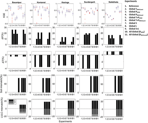
KGE exhibits significant variability in model response among the 11 experiments across sub-catchments. The median of KGE suggests the benchmark produced the best performance at Basantpur, Kantamal and Sundergarh, while it performed moderately for the rest sub-catchments. The median KGE values for the benchmark simulation across sub-catchments Ba, Ka, Ke, Sa and Su are 0.80, 0.74, 0.46, 0.66 and 0.25, respectively. The simulation driven by GPM rainfall (exp3) outperformed the benchmark simulation and simultaneously produced the best performance at two sub-catchments (Kantamal and Kesinga), while slight to significant deterioration in KGE is observed for the rest of the sub-catchments. Conversely, the other global source of precipitation, ERA5-Land (exp4), showed a relatively much poorer performance with decreased KGE in every sub-catchment. Simulations using ERA5-Land temperatures (exp2) performed well across all sub-catchments, with a slight decline in KGE as compared to the reference simulation. Simulations using both precipitation and temperature from global sources (exp5,6) caused more decline in KGE than using either of them as a sole input from global sources. In particular, the combination of ERA5-Land precipitation and temperature (exp6) showed significant deterioration in all sub-catchments. The global soil map from SoilGrids (exp7) yielded KGE values almost identical to (lying almost in the same interquartile range) the benchmark at four sub-catchments, suggesting a nonsignificant change in overall model performance. In contrast, the use of the global land cover map from ESA CCI (exp8) showed a deterioration in model performance in four sub-catchments while producing the best performance in one sub-catchment (Salebhata). The impact of replacing all local datasets with global datasets in the VIC model (exp10,11) varies across sub-catchments. However, in most instances, experiments using all global datasets (exp10,11) showed better performances than experiments using only precipitation and temperature from global sources (exp4,10), implying that global soil and LULC in exp10 and 11 compensate for the poor performances in exp4 and 10.

On some occasions, we observe that KGE enables a finer distinction between experiments, revealing clear trends arising from the influence of the different input datasets – varying, however, across sub-catchments (see Fig. S2 in the Supplementary material). For instance, at Basantpur, we observe a finer distinction between experiments driven by IMD precipitation (exp1,2,7,8,9) and global precipitation (exp3,4,5,6,10,11). The latter yielded much lower KGE values than the experiments using IMD precipitation, emphasizing the importance of local precipitation estimates in this sub-catchment. At Kesinga, simulations involving GPM precipitation (exp3,5,10) produced the best results, whereas simulations using reanalysis forcings (exp4,6,11) showed the maximum deterioration in KGE. Simulations using local forcings perform moderately in this sub-catchment. At Salebhata, we observe that all experiments involving global land cover (exp8,9,10,11) outperformed the experiments involving local land cover (exp1,2,3,4,5,6,7).

4.2 Factors causing changes in model performance due to different data sources

4.2.1 Weather datasets

Figure 5 (bottom panels) shows the percentage change in the input factors (precipitation, temperature, soil and land cover) obtained from global sources relative to the datasets from local sources. Each of the experiments (on the x-axis) in the bottom panel represented by the bar plots for different factors corresponds to the same experiment numbers in the top panel showing box plots of KGE values. The performance produced by each experiment (shown by KGE in the top panel) can be related to all four factors of the corresponding experiment to understand which factor is responsible for the change in the KGE values.

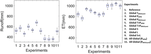
Both global rainfall datasets, GPM and ERA5-Land, overestimated the daily rainfall values when compared to IMD rainfall across sub-catchments. However, the decline in KGE is mainly caused while using ERA5-Land rainfall datasets. Moderate to large overestimation (11–20%) in ERA5-Land rainfall produced consistently poor performance (see exp4 in Fig. 5). A 5% increase in GPM annual rainfall at Kesinga outperformed the benchmark simulation by improving slight positive biases and variability (not shown here) in streamflow, implying that precipitation estimates of IMD resulted in slight overestimation in discharge at this sub-catchment. However, to understand the factor causing a reduction in discharge despite the 5% increase in GPM precipitation, we assessed the water balance components (Fig. 6). We observe that replacing IMD precipitation with GPM induced more evapotranspiration, thereby reducing total runoff. The annual averages of runoff and Evapotranspiration (ET) for the rest of the sub-catchments are shown in the Supplementary material (Fig. S3). Further increases (16–26%) in GPM annual rainfall have largely overestimated the streamflow at Basantpur, Sundergarh and Salebhata.

Figure 6. Annual average of runoff and evapotranspiration at Basantpur for all experiments. In the legend, T, P, S and L are temperature, precipitation, soil and LULC, respectively. Note that the precipitation varies across experiments.

The decline in KGE while using ERA5-Land temperatures is attributed to the decrease in average temperature by 0.5–4.8% that tends to overestimate the discharge. Decreases in maximum temperature have reduced the evapotranspiration, thereby increasing runoff (see Fig. S3). Note that both maximum and minimum temperatures are used as inputs in the model; however, for the sake of simplicity, only the change in the average temperatures is shown in Fig. 5. The overestimating tendency of both precipitation and temperatures from ERA5Land caused further deterioration in exp 6.

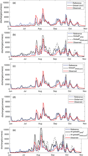
Figure 7 shows a visual comparison between observed and simulated discharges of the experiments at Basantpur to understand how prediction of discharge differs between experiments and to visually assess the model performance. A visual comparison of observed and simulated discharge for the rest of the sub-catchments is provided in the Supplementary material (Figs. S4–S7). Figure 7 clearly illustrates that at Basantpur, benchmark simulation using IMD rainfall closely matches the observed flow, whereas some overestimation is observed in simulations driven by GPM (exp3) and ERA5-Land (exp4) rainfall. In this sub-catchment, simulations driven by reanalysis precipitation, ERA5-Land (exp4,6,11), have performed better than those using GPM precipitation (exp3,5,10). This is because ΔP for GPM (303 mm) is higher than for ERA5Land (219 mm), therefore relative overestimation is higher in GPM.

Figure 7. Comparison of daily observed discharge and ensemble mean of simulated discharge of experiments at Basantpur using (a) precipitation from GPM, ERA5-land and IMD (reference); (b) temperature from ERA5-Land and IMD (reference); (c) soil from SoilGrids and local soil (reference); (d) LULC from ESA CCI and local LULC (reference); (e) all global datasets and all local datasets (reference), averaged for the years 2014–2016. In order to show the details of the hydrographs, they are zoomed in to the monsoon (wet) months; results for other sub-catchments are similar and can be found in the Supplementary material (Figs. S4–S7).

4.2.2 Soil and land cover datasets

A significant difference in the granularity of data is clearly visible in the soil maps, which ranges from 83 to 97% across sub-catchments (Fig. 2). Loam and some percentage of clay in the local soil map is mapped as clay loam in SoilGrids. Despite a significant variation in the percentage of soil textures and spatial distribution in both soil maps, we observe nonsignificant changes in model performance, i.e. they closely represent the benchmark flows which are simulated using local soil. This is because the mismatch in soil classification occurs among soil types with comparable hydraulic properties, thereby having little influence on the predicted discharge. Figure 7 clearly illustrates that discharge patterns using global soil closely represent the benchmark flows and observed flows.

The global land cover map has an underestimating tendency primarily due to reduced barren grounds in ESA CCI, thereby deteriorating the model performance across the sub-catchments except in Salebhata. Under-prediction in discharge might also be caused due to agricultural expansion (10–21%) through increased ET (Fig. S3). However, the global map captured the low flows better than the local land cover across the sub-catchment, as can be observed from Fig. 6. This indicates ESA CCI mainly under-predicted the peak flows. At Salebhata, reduction in barren ground by 17% and expansion in cropland by 24% in the global land cover (exp8,9) led it to outperform all other experiments related to local land cover. The local land cover seems to have over-predicted the flows at this sub-catchment. Interestingly, using all model inputs from global sources, the model did not yield the worst KGE values as we hypothesized. This is because simulation using all global inputs includes global land cover that compensates for the poor performance due to the overestimating tendency of global weather inputs, specifically precipitation.

5 Discussion

Although we conducted the analysis for selected sub-basins to avoid the effects of a major dam/reservoir in the middle reach of the basin, the sub-basins analysed are also affected by human intervention, and their observed streamflow is controlled by minor reservoirs and dams. This will affect the VIC model simulations, especially in the smaller sub-catchments, which is possibly the reason behind the poor benchmark performance at Kesinga and Salebhata, despite being calibrated using local datasets. Moreover, non-consideration of groundwater recharge and irrigation in the model could also affect the performance. This is in line with some studies in the literature (Mishra et al. 2008, Kneis et al. 2014) wherein the calibrated hydrological models yielded poor performance in smaller sub-basins of Mahanadi.

Precipitation estimates from both GPM IMERG and ERA5-Land have overestimated the discharge. Overestimation using IMERG rainfall estimates is in line with the findings of Beria et al. (2017) and Zubieta et al. (2016). For instance, Beria et al. (2017) found overestimation in low runoff at Hirakud sub-catchment of Mahanadi River basin during the 2014 monsoon. Peak discharge simulated by GPM IMERG, although well captured, showed an overestimation which contradicts the findings of Beria et al. (2017), who found that the runoff peaks are underreported. Gilewski and Nawalany (2018) also reported overestimation of extreme rainfall events by GPM in monsoon-dominated regions. ERA5-Land is a recent advancement among the ECMWF reanalysis products, therefore very limited studies using it exist worldwide. A recent study by Gao et al. (2020) evaluated the state-of-the-art gridded rainfall products, wherein IMERG outperforms all reanalysis datasets including ERA5-Land at both hourly and daily scales. As reported in the literature (Shah and Mishra 2014a, Dhanya and Villarini 2017, Mahto and Mishra 2019), the majority of reanalysis products including ERA5 show a consistent increasing trend during Indian monsoons and largely fail to reproduce observed flows in the monsoon season in most parts of India. This finding correlates with our analysis as ERA5-Land overestimated the discharge at all sub-basins and 90% of rainfall is received during the monsoon. This overestimation in discharge using both IMERG and ERA5-Land can directly be linked to the overestimation of rainfall estimates at these sub-catchments, as also reported by Mahto and Mishra (2019) and Zubieta et al. (2016). For instance, Zubieta et al. (2016) found over- and under-prediction in runoff when the rainfall estimates are over- and underestimated, respectively. However, much larger overestimation is observed in reanalysis products than satellite products, as reanalysis models generate too much light rainfall. IMD gridded rainfall products are acquired from a reasonably good network of raingauge observations spread across the country, hence they might be expected to capture average daily events more accurately. However, this also depends on how well maintained and calibrated the instrumentations are. Moreover, the very high resolution of IMERG rainfall products might be a reason it produces better simulations than IMD rainfall, which is relatively coarse. Maximum and minimum temperatures from ERA5-Land had overestimated discharge – less, however, than the overestimation caused by precipitation from ERA5-Land. Generally, temperature exhibits smaller biases compared to precipitation, as also found by Essou et al. (2016). Overestimation of monsoon runoff caused by an increase in maximum temperature is also reported by Mahto and Mishra (2019) and Ghodichore et al. (2018) for ERA5 and other reanalysis products over India.

Global soil texture information from SoilGrids of resolution 1 km has resulted in a comparable performance at all sub-basins. In line with our findings, Yeste et al. (2020) obtained good hydrological responses using textural information from SoilGrids 1km in the north of the Iberian Peninsula. In contrast, Tarawneh et al. (2016) found that the local detailed soil map produced much better simulations than the global soil map. However, the difference in the impact of using global versus local soil maps on the simulated discharge depends on the difference between the soil textures present in the two sources. For instance, replacing local soil with global did not have much impact on simulations for Strömqvist et al. (2009) and Faramarzi et al. (2015). Strömqvist et al. (2009) found that a change of soil type from clay to loam (both having similar hydraulic properties) had little effect on streamflow. The global LULC overall tends to under-predict the discharge. However, the global LULC map, when used across the rest of scenarios with other inputs having an overestimating tendency (such as global rainfall and global temperature), compensates for the positive bias and improves the model performance. As also found in our study, the global LULC map from USGS improved the biases; however, it did not significantly improve the streamflow, and Tarawneh et al. (2016) found the global LULC map had the least influence on model performance.

VIC (and other land surface models) have a large number of parameters, which often contributes to uncertainties in the simulated discharge, and there may exist multiple model parameter sets that can yield equally good results, or behavioral model outputs which can lead to widely divergent results under novel conditions (Her et al. 2019). Therefore, using 250 behavioral VIC models while capturing the hydrological responses, driven by datasets of multiple sources, makes our analysis more robust and reliable. In contrast, employing only one parameter set could have led to improper representation of hydrological processes, thus making it difficult to disentangle the impacts of using these datasets on discharge predictions.

Model performances using all these global datasets vary from one sub-catchment to another, which might be due to the regional differences in quality of these datasets, particularly the satellite datasets. But to clearly understand whether the poor performance at some stations is due to limitations in input datasets or due to the process representations in the VIC model, other land surface models or hydrological models should be used.

It is worth mentioning that the purpose of this paper is to understand the impact of local versus global input data on the model behaviour or, in other words, to understand how reliable these new global datasets are in producing a comparable hydrological model performance when compared against local observations. The analysis presented here is about the impact of those products on model prediction and we chose a model that is calibrated locally as a reference point (as we have the monitoring capability), to remove any potential biases from local conditions. Also, model evaluation for different combinations is done in a different period compared to the calibration. The locally calibrated model is therefore our benchmark, and we further want to understand how much the model using global input datasets deviates from our benchmark. Note that we could have performed the same experiments with the default model, which would likely contain biased results because of uncalibrated parameter sets.

An alternative way to approach this analysis would have been by calibrating the VIC model individually for each input combination. In this case, the optimal performance of VIC for each combination would have been achieved and the impact of those combinations would have been translated to the values obtained for each parameter in VIC. However, such an approach was not chosen in this study and it is beyond the scope of our original goal to directly observe the impacts of input calibration on the model output.

6 Conclusions

In this study, we seek to understand the impacts of using new high-resolution global datasets as inputs in a land surface model, VIC, on hydrological responses of the Mahanadi River basin. To elucidate these impacts, we frame different model experiments using precipitation, temperature, soil, and land use datasets from both local and global products and perform a comprehensive evaluation of the model performance. Global precipitation datasets were acquired from GPM IMERG and ERA5-Land and a global temperature dataset was obtained from ERA5-Land. Global soil and land cover data are obtained from SoilGrids and ESA CCI, respectively.

From the analysis of outcomes, the following key conclusions can be drawn:

1. The model experiment using all local datasets (reference) produced the best or comparable simulation results at three out of five sub-catchments in the evaluation period. Note that the calibration using all local datasets is performed in a completely different period (1990–2000). Replacing local precipitation with IMERG yielded the best KGE in two sub-catchments, and replacing the local land cover map with the ESA CCI map produced the best result in one sub-catchment.

2. Both satellite and reanalysis products (GPM and ERA5-Land, respectively) overestimated daily rainfall estimates, which caused over-prediction in discharge. However, the overall performance of GPM is better than that of ERA5-Land and it could be used as an alternative to local precipitation estimates from IMD. ERA5-Land seems to overestimate significantly in all sub-catchments.

3. Maximum and minimum temperatures from ERA5-Land slightly overestimated discharge; however, overall it showed a moderate performance.

4. Global soil from SoilGrids produced a comparable performance in all sub-basins. Some changes in soil textures with similar hydraulic properties have little impact on discharge in this region.

5. The global land cover map from ESA CCI tends to underestimate the flows in all sub-catchments, primarily due to reduced barren grounds. However, the low flows are better captured compared to the local map, as using all local datasets in benchmark simulation overestimated the low flows.

6. Our findings do not support our hypothesis that driving VIC using all input datasets from global sources (exp8 and 11) will show maximum decline in KGE. Rather, exp8 and 11 outperformed experiments using only meteorological forcings (precipitation; maximum and minimum temperature) from global sources and soil and land cover from local sources. This is because the underestimating tendency of global land cover and the overestimating tendency of global forcings ultimately improve the biases in streamflows.

7. The ranking of the global products most suitable for this region is as follows: SoilGrids, GPM rainfall, ER5-Land temperatures, ESA CCI land cover and ERA5-Land rainfall. However, the effects of inclusion of different combinations of these datasets may vary the model predictions.

These results are based on an analysis of three years (2014–2016), primarily due to the unavailability of local maximum and minimum temperature records from IMD. Moreover, retrospectively processed fully GPM-based IMERG data starting from 1998 became available during the later stage of our study. A longer period would likely result in an improved evaluation of such products. However, a comparison of CDF of rainfall and minimum/maximum temperature from 1990 to 2014 (long-term data availability from IMD) against those for 2014–2016 (analysed in this study) showed that the pattern of both daily rainfall and temperature (maximum and minimum) values in the two periods are very similar (data not shown). We observed that the three years of rainfall data (2014–2016) is slightly drier than the 13 years of rainfall data (1990–2014) with no such differences in the higher rainfall values in both datasets. Both daily minimum and maximum temperatures of the three-year dataset are slightly warmer than those of the 13-year dataset. Future work should involve a long-term hydrological analysis using these datasets, and it is also essential to test the global products, especially rainfall and temperature, at their native resolution against IMD observations, which would provide an in-depth exploration of these new datasets.

Disclosure statement

No potential conflict of interest was reported by the authors.

Supplementary material

Supplemental data for this article can be accessed online at https://doi.org/10.1080/02626667.2023.2193700

Data availability statement

The DEM is freely available from https://bhuvan-app3.nrsc.gov.in/data/download/index.php. The unit hydrograph is adapted from https://vic.readthedocs.io/en/vic.4.2.d/Documentation/Routing/UH/. Daily gridded rainfall and maximum and minimum temperature are freely available from http://www.imdpune.gov.in/Clim_Pred_LRF_New/Grided_Data_Download.html. Wind speed data is freely available from https://psl.noaa.gov/cgibin/db_search/DBSearch.pl?Dataset=NCEP±Reanalysis±Daily±Averages. Observed discharge data are available from http://cwc.gov.in/. The source code for VIC-3L version 4.2.d is available from https://github.com/UW-Hydro/VIC/releases/tag/VIC.4.2.d. Soil textural information to prepare the soil map of soilGrids is derived from https://soilgrids.org/. The ESA CCI land cover map was downloaded from www.esa-landcover-cci.org/. The ERA5-Land precipitation and temperature products were obtained from https://cds.climate.copernicus.eu/cdsapp#!/dataset/reanalysis-era5-land?tab=form.

Additional information

Funding

This work was funded by the BEMUSED project funded by Natural Environment Research Council (NERC; grant number NE/R004897/1).

Appendix.

The spatial resolutions of all rainfall and temperature datasets including IMD, used as inputs in VIC are kept at a model resolution of 0.05°. However, to enable comparisons, precipitation datasets from IMERG and ERA5-Land are re-gridded to the spatial resolution of the reference precipitation dataset, IMD (0.25° × 0.25°). To achieve this, IMERG and ERA5-Land gridded precipitation values (0.1°) are first resampled to 0.05°and then spatially averaged to 0.25° to match each target grid of IMD. A similar approach has been applied in other studies (Prakash et al. 2018, Essou et al. 2016, Mahto and Mishra 2019). Figure A1 shows spatial distributions of mean annual rainfall over Mahanadi River basin for all three datasets averaged for the time period 2014–2016 at a common resolution of 0.25°.

We use two skill measures to statistically evaluate the different precipitation and temperature datasets: Pearson correlation coefficient (r) (Equation A1), and percentage bias (PBIAS) (Equation A2).

(A1) $r={\left(\frac{{\sum }_{i=1}^n\left(O-\bar{O}\right)(P-\bar{P})}{\sqrt{{\sum }_{i=1}^n{\left(O-\bar{O}\right)}^2{\sum }_{i=1}^n{\left(P-\bar{P}\right)}^2}}\right)}^2$(A1)

(A2) $PBIAS=\frac{{\sum }_{i=1}^n\left(O-P\right).100}{{\sum }_{i=1}^{n}O}$(A2)

where $O$ and $P$ are the observed (IMD) and predicted (IMERG and ERA5-Land) rainfall and temperature values, respectively, and $\bar{O}$ and $\bar{P}$ are the observed mean and predicted mean. n is the number of data points. The skill measures for the global rainfall and temperature products against locally available data from IMD are computed and represented spatially for the entire Mahanadi River basin averaged for the period 2014–2016, shown in Figs. A2 and A3.

The correlation pattern suggests IMERG precipitation is more correlated to the reference precipitation, IMD, in the basin, with an average correlation of 0.7 compared to the average ERA5-Land correlation of 0.6. Spatial bias maps suggest similar bias pattern in both IMERG and ERA5-Land precipitation in almost the entire basin and both rainfall products are found to be positively biased, indicating overestimation of rainfall values. But the overestimation is higher in IMERG, with an average (spatially) positive bias of 21%, than in ERA5-Land with an average of 17%. Temporal correlation between IMD and IMERG is in the range of 0.72–0.86 across the sub-basins which is higher than ERA5-Land (0.59–0.79) (not shown here).

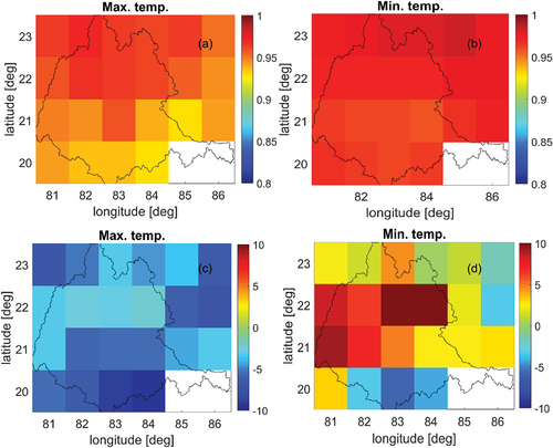
Daily maximum and minimum temperatures from ERA5-Land at a spatial resolution 0.1° are re-gridded to 1°, the spatial resolution of IMD maximum and minimum temperatures. Owing to the coarse resolution of IMD temperatures, there are only few grids in the entire basin. So, we compared maximum and minimum temperatures from ERA5-Land and IMD (see Fig. A4) for the entire river basin. Figure A3 shows spatial distributions of maximum and minimum temperatures over Mahanadi River basin from ERA5-Land and IMD averaged for the time period 2014–2016 at a common resolution of 0.25°. Both maximum and minimum temperatures from ERA5-Land showed high spatial correlation, with an average of 0.93 and 0.96, respectively (Fig. A4). The temporal correlation coefficient between the daily time series of IMD maximum temperature and ERA5-Land maximum temperature is 0.94, and that between IMD minimum temperature and ERA5-Land minimum temperature is 0.95. Spatial RMSE shows that the overall error in the maximum temperature (2.39) is greater than that of the minimum temperature (1.6). Spatial bias maps indicate that the maximum temperature in ERA5-Land is mostly negatively biased, i.e. it has a tendency to underestimate, whereas the minimum temperature is mostly positively biased, i.e. it has a tendency to overestimate. The average bias in the maximum temperature and minimum temperature across the basin is −5% and 4%, respectively.

Figure A1. Spatial distributions of mean annual rainfall over Mahanadi River basin averaged for the time period 2014–2016, derived from IMD gauge-based, IMERG, and ERA5-LAND precipitation datasets.

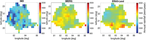
Figure A2. Spatial distributions of (a) correlation between GPM and IMD; (b) correlation between ERA5-Land and IMD; (c) PBIAS of GPM against IMD; and (d) PBIAS of ERA5-Land and IMD daily rainfall over Mahanadi River for 2014–2016.

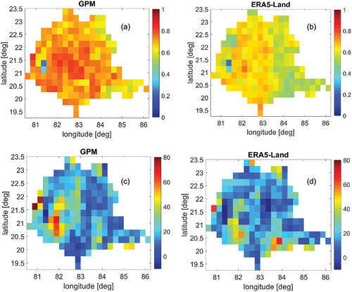
Figure A3. Spatial distributions of mean daily maximum temperature derived from (a) IMD and (b) ERA5-LAND; and spatial distributions of mean daily minimum temperature derived from (c) IMD and (d) ERA5-Land, averaged for the period 2014–2016.

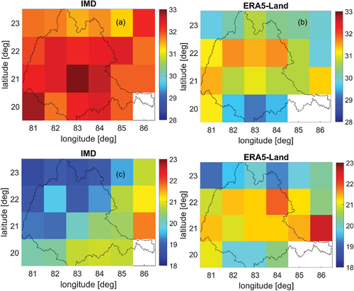
Figure A4. Spatial distributions of (a) correlation between maximum temperature from ERA5-Land and IMD; (b) correlation between minimum temperature from ERA5-Land and IMD; (c) PBIAS between maximum temperature from ERA5-Land and IMD; and (d) PBIAS between maximum temperature from ERA5-Land and IMD, over Mahanadi River averaged for 2014–2016.

References

- Bennett, K.E., et al., 2018. Global sensitivity of simulated water balance indicators under future climate change in the Colorado Basin. Water Resources Research, 54 (1), 132–149. doi:10.1002/2017WR020471
- Beria, H., et al., 2017. Does the GPM mission improve the systematic error component in satellite rainfall estimates over TRMM? An evaluation at a pan-India scale. Hydrology and Earth System Sciences, 21 (12), 6117–6134. doi:10.5194/hess-21-6117-2017
- Bierkens, M.F.P., et al., 2015. Hyper-resolution global hydrological modelling: what is next?: “Everywhere and locally relevant” M. F. P. Bierkens et al. Invited commentary. Hydrological Processes, 29 (2), 310–320. doi:10.1002/hyp.10391
- Bosmans, J.H.C., et al., 2017. Hydrological impacts of global land cover change and human water use. Hydrology and Earth System Sciences, 21 (11), 5603–5626. doi:10.5194/hess-21-5603-2017
- Chen, Z., et al., 2020. Global land monsoon precipitation changes in CMIP6 projections. Geophysical Research Letters, 47 (14). doi:10.1029/2019GL086902
- Cherkauer, K.A. and Lettenmaier, D.P., 1999. Hydrologic effects of frozen soils in the upper Mississippi River basin. Journal of Geophysical Research: Atmospheres, 104 (D16), 19599–19610. doi:10.1029/1999JD900337
- Clark, M.P., et al., 2015. Hydrological partitioning in the critical zone: recent advances and opportunities for developing transferable understanding of water cycle dynamics. Water Resources Research, 1–28. doi:10.1002/2015WR017096.
- Collischonn, W., et al., 2007. The MGB-IPH model for large-scale rainfall-runoff modelling. Hydrological Sciences Journal, 52 (5), 878–895. doi:10.1623/hysj.52.5.878
- Connor, R., 2016. The United Nations world water development report 2015: water for a sustainable world. UNESCO publishing.
- Cosby, B.J., et al., 1984. A statistical exploration of the relationships of soil moisture characteristics to the physical properties of soils. Water Resources Research, 20 (6), 682–690. doi:10.1029/WR020i006p00682
- Dai, Y., et al., 2019. A review of the global soil property maps for Earth system models. Soil, 5 (2), 137–158. doi:10.5194/soil-5-137-2019
- Demaria, E.M., Nijssen, B., and Wagener, T., 2007. Monte Carlo sensitivity analysis of land surface parameters using the variable infiltration capacity model. Journal of Geophysical Research, 112 (11), 1–15. doi:10.1029/2006JD007534
- Dembélé, M., et al., 2020. Suitability of 17 rainfall and temperature gridded datasets for largescale hydrological modelling in West Africa. Hydrology and Earth System Sciences, 1–39. doi:10.5194/hess-2020-68
- Dhanya, C.T. and Villarini, G., 2017. An investigation of predictability dynamics of temperature and precipitation in reanalysis datasets over the continental United States. Atmospheric Research, 183, 341–350. doi:10.1016/j.atmosres.2016.09.017
- Essou, G.R.C., et al., 2016. Can precipitation and temperature from meteorological reanalyses be used for hydrological modeling? Journal of Hydrometeorology, 17 (7), 1929–1950. doi:10.1175/JHM-D-15-0138.1
- Faramarzi, M., et al., 2015. Setting up a hydrological model of Alberta: data discrimination analyses prior to calibration. Environmental Modelling & Software, 74, 48–65. doi:10.1016/j.envsoft.2015.09.006
- Fisher, R.A. and Koven, C.D., 2020. Perspectives on the future of land surface models and the challenges of representing complex terrestrial systems. Journal of Advances in Modeling Earth Systems, 12 (4). doi:10.1029/2018MS001453
- Gao, H., et al., 2010. Water budget record from Variable Infiltration Capacity (VIC) model. Algorithm Theor. Basis Doc. Terr. Water Cycle Data Rec., (Vic), 120–173 [online]. Available from: http://scholar.google.com/scholar?hl=en&btnG=Search&q=intitle:Water+Budget+Record+from+Variable+Infiltration+Capacity+(+VIC+)+Model#2.
- Gao, Z., et al., 2020. Comprehensive comparisons of state-of-the-art gridded precipitation estimates for hydrological applications over southern China. Remote Sensing, 12 (23), 1–20. doi:10.3390/rs12233997
- Ghodichore, N., et al., 2018. Reliability of reanalyses products in simulating precipitation and temperature characteristics over India. Journal of Earth System Science, 127 (8), 1–21. doi:10.1007/s12040-018-1024-2
- Gilewski, P. and Nawalany, M., 2018. Inter-comparison of Rain-Gauge, Radar, and Satellite (IMERG GPM) precipitation estimates performance for rainfall-runoff modeling in a mountainous catchment in Poland. Water (Switzerland), 10 (11), 1–23. doi:10.3390/w10111665
- Gou, J., et al., 2020. Sensitivity analysis-based automatic parameter calibration of the VIC model for streamflow simulations over China. Water Resources Research, 56 (1), 1–19. doi:10.1029/2019WR025968
- Gupta, H.V., et al., 2009. Decomposition of the mean squared error and NSE performance criteria: implications for improving hydrological modelling. Journal of Hydrology, 377 (1–2), 80–91. doi:10.1016/j.jhydrol.2009.08.003
- Hengl, T., et al., 2017. SoilGrids250m: global gridded soil information based on machine learning. PLoS One, 12 (2), e0169748.
- Her, Y., et al., 2019. Uncertainty in hydrological analysis of climate change: multi-parameter vs. multi-GCM ensemble predictions. Scientific Reports, 9 (1), 1–22. doi:10.1038/s41598-019-41334-7
- Huffman, G.J., et al., 2007. The TRMM multisatellite precipitation analysis (TMPA): quasi-global, multiyear, combined-sensor precipitation estimates at fine scales. Journal of Hydrometeorology, 8 (1), 38–55. doi:10.1175/JHM560.1
- Huffman, G.J. et al., 2018. NASA global precipitation measurement (GPM) integrated multi-satellite retrievals for GPM (IMERG). Algorithm Theoretical Basis Document (ATBD) Version, 4.
- Huffman, G.J., Bolvin, D.T., and Nelkin, E.J., January 2015. Day 1 IMERG final run release notes. 1–9 [online]. Available from: https://pmm.nasa.gov/sites/default/files/document_files/IMERG_FinalRun_Day1_release_notes.pdf.
- Jiang, L. and Yu, L., July 2018. Analyzing land use intensity changes within and outside protected areas using ESA CCI-LC datasets. Global Ecology and Conservation, 20. doi:10.1016/j.gecco.2019.e00789
- Jin, L., et al., 2018. Simulating climate change and socio-economic change impacts on flows and water quality in the Mahanadi River system, India. Science of the Total Environment, 637–638, 907–917. doi:10.1016/j.scitotenv.2018.04.349
- Joseph, J., et al., 2018. Hydrologic impacts of climate change: comparisons between hydrological parameter uncertainty and climate model uncertainty. Journal of Hydrology, 566 (September), 1–22. doi:10.1016/j.jhydrol.2018.08.080
- Kneis, D., Chatterjee, C., and Singh, R., 2014. Evaluation of TRMM rainfall estimates over a large Indian river basin (Mahanadi). Hydrology and Earth System Sciences, 18 (7), 2493–2502. doi:10.5194/hess-18-2493-2014
- Knoben, W.J.M., Freer, J.E., and Woods, R.A., 2019. Technical note: inherent benchmark or not? Comparing Nash-Sutcliffe and Kling-Gupta efficiency scores. Hydrology and Earth System Sciences, 23 (10), 4323–4331. doi:10.5194/hess-23-4323-2019
- Krpec, P., Horáček, M., and Šarapatka, B., February 2020. A comparison of the use of local legacy soil data and global datasets for hydrological modelling a small-scale watersheds: implications for nitrate loading estimation. Geoderma, 377, 114575. doi:10.1016/j.geoderma.2020.114575
- Liang, X., et al., 1994. A simple hydrologically based model of land surface water and energy fluxes for GSMs. Journal of Geophysical Research, 99 (D7), 14415–14428. doi:10.1029/94JD00483
- Liu, Y., et al., 2011. Impacts of land-use and climate changes on hydrologic processes in the Qingyi River Watershed, China. Journal of Hydrologic Engineering, 18 (11), 1495–1512. doi:10.1061/(asce)he.1943-5584.0000485
- Lohmann, D.A.G., Nolte-Holube, R., and Raschke, E., 1996. A large-scale horizontal routing model to be coupled to land surface parametrization schemes. Tellus A, 48 (5), 708–721. doi:10.3402/tellusa.v48i5.12200
- Mahto, S.S. and Mishra, V., 2019. Does ERA-5: outperform other reanalysis products for hydrologic applications in India? Journal of Geophysical Research: Atmospheres, 124 (16), 9423–9441. doi:10.1029/2019JD031155
- Mishra, V., et al., 2020. Does comprehensive evaluation of hydrological models influence projected changes of mean and high flows in the Godavari River basin? Climatic Change, 163 (3), 1187–1205. doi:10.1007/s10584-020-02847-7
- Mishra, N., Aggarwal, S.P., and Dadhwal, V.K., 2008. Macroscale hydrological modelling and impact of land cover change on stream flows of the Mahanadi River basin. A Master thesis submitted to Andhra University, Indian Institute of Remote Sensing (National Remote Sensing Agency) Dept. of Space, Govt. of India.
- Mujumdar, P.P., 2015. Share data on water resources. Nature, 521 (7551), 151–152.
- Muñoz-Sabater, J., et al., 2021. ERA5-Land: a state-of-the-art global reanalysis dataset for land applications. Earth System Science Data, 13 (9), 4349–4383.
- Naha, S., Rico-Ramirez, M.A., and Rosolem, R., 2021. Quantifying the impacts of land cover change on hydrological responses in the Mahanadi river basin in India. Hydrology and Earth System Sciences, 25 (12), 6339–6357. doi:10.5194/hess-25-6339-2021
- Pai, D.S., et al., 2014. Development of a new high spatial resolution (0.25° × 0.25°) long period (1901-2010) daily gridded rainfall data set over India and its comparison with existing data sets over the region. Mausam, 65 (1), 1–18. doi:10.54302/mausam.v65i1.851
- Prakash, S., et al., 2018. A preliminary assessment of GPM-based multi-satellite precipitation estimates over a monsoon dominated region. Journal of Hydrology, 556, 865–876. February. doi:10.1016/j.jhydrol.2016.01.029.
- Rawls, W.J., Gimenez, D., and Grossman, R., 1998. Use of soil texture, bulk density, and slope of the water retention curve to predict saturated hydraulic conductivity. Transactions of the ASAE, 41 (4), 983. doi:10.13031/2013.17270
- Reynolds, C.A., Jackson, T.J., and Rawls, W.J., 2000. Estimating soil water-holding capacities by linking the food and agriculture organization soil map of the world with global pedon databases and continuous pedotransfer functions. Water Resources Research, 36 (12), 3653–3662. doi:10.1029/2000WR900130
- Rodell, M., et al., 2005. Evaluation of 10 methods for initializing a land surface model. Journal of Hydrometeorology, 6 (2), 146–155. doi:10.1175/JHM414.1
- Rodriguez, D.A. and Tomasella, J., 2016. On the ability of large-scale hydrological models to simulate land use and land cover change impacts in Amazonian basins. Hydrological Sciences Journal, 61 (10), 1831–1846. doi:10.1080/02626667.2015.1051979
- Rodríguez, E., et al., 2020. Combined use of local and global hydro meteorological data with hydrological models for water resources management in the Magdalena - Cauca Macro Basin – Colombia. Water Resources Management, 34 (7), 2179–2199. doi:10.1007/s11269-019-02236-5
- Shah, R. and Mishra, V., 2014a. Evaluation of the reanalysis products for the Monsoon season droughts in India. Journal of Hydrometeorology, 15 (4), 1575–1591. doi:10.1175/jhm-d-13-0103.1
- Shah, R. and Mishra, V., 2014b. Evaluation of the reanalysis products for the Monsoon season Droughts in India. Journal of Hydrometeorology, 15 (4), 1575–1591. doi:10.1175/jhm-d-13-0103.1
- Sharifi, E., Steinacker, R., and Saghafian, B., 2016. Assessment of GPM-IMERG and other precipitation products against gauge data under different topographic and climatic conditions in Iran: preliminary results. Remote Sensing, 8 (2). doi:10.3390/rs8020135
- Sivasena Reddy, A. and Janga Reddy, M., 2015. Evaluating the influence of spatial resolutions of DEM on watershed runoff and sediment yield using SWAT. Journal of Earth System Science, 124 (7), 1517–1529. doi:10.1007/s12040-015-0617-2
- Sterling, S.M., Ducharne, A., and Polcher, J., 2013. The impact of global land-cover change on the terrestrial water cycle. Nature Climate Change, 3 (4), 385–390. doi:10.1038/nclimate1690
- Strömqvist, J., et al., September 2009. Using recently developed global data sets for hydrological predictions. IAHS-AISH Publication, 333, 121–127.
- Sungmin, O., et al., 2017. Evaluation of GPM IMERG early, late, and final rainfall estimates using WegenerNet gauge data in southeastern Austria. Hydrology and Earth System Sciences, 21 (12), 6559–6572. doi:10.5194/hess-21-6559-2017
- Tang, G., et al., 2020. Have satellite precipitation products improved over last two decades? A comprehensive comparison of GPM IMERG with nine satellite and reanalysis datasets. Remote Sensing of Environment, 240, 111697. September. doi:10.1016/j.rse.2020.111697.
- Tarawneh, E., Bridge, J., and Macdonald, N., 2016. A pre-calibration approach to select optimum inputs for hydrological models in data-scarce regions. Hydrology and Earth System Sciences, 20 (10), 4391–4407. doi:10.5194/hess-20-4391-2016
- Van Den Hurk, B., et al., 2011. Acceleration of land surface model development over a decade of glass. Bulletin of the American Meteorological Society, 92 (12), 1593–1600. doi:10.1175/BAMS-D-11-00007.1
- Voisin, N., Wood, A.W., and Lettenmaier, D.P., 2008. Evaluation of precipitation products for global hydrological prediction. Journal of Hydrometeorology, 9 (3), 388–407. doi:10.1175/2007JHM938.1
- Wood, E.F., et al., 2011. Hyperresolution global land surface modeling: meeting a grand challenge for monitoring Earth’s terrestrial water. Water Resources Research, 47 (5), doi:10.1029/2010WR010090
- Yanto, L.B., Kasprzyk, J., and Kasprzyk, J., 2017. Hydrological model application under data scarcity for multiple watersheds, Java Island, Indonesia. Journal of Hydrology: Regional Studies, 9, 127–139. doi:10.1016/j.ejrh.2016.09.007
- Yeste, P., et al., 2020. Integrated sensitivity analysis of a macroscale hydrologic model in the North of the Iberian Peninsula. Journal of Hydrology, 590 (September 2019), 125230. doi:10.1016/j.jhydrol.2020.125230
- Zeng, X., 2002. Global vegetation root distribution for land modeling. Journal of Hydrometeorology, 2 (5), 525–530. doi:10.1175/1525-7541(2001)002<0525:GVRDFL>2.0.CO;2
- Zhao, R.J., et al., The Xinanjiang model hydrological forecasting proceedings Oxford symposium, IASH, 1980.
- Zubieta, R., et al., 2016. Hydrological modeling of the Peruvian-Ecuadorian Amazon basin using GPM-IMERG satellite-based precipitation dataset. Hydrology and Earth System Sciences, 1–21. doi:10.5194/hess-2016-656