Clustering of match running and performance indicators to assess between- and within-playing position similarity in professional rugby league

ABSTRACT

This study aimed to determine the similarity between and within positions in professional rugby league in terms of technical performance and match displacement. Here, the analyses were repeated on 3 different datasets which consisted of technical features only, displacement features only, and a combined dataset including both. Each dataset contained 7617 observations from the 2018 and 2019 Super League seasons, including 366 players from 11 teams. For each dataset, feature selection was initially used to rank features regarding their importance for predicting a player’s position for each match. Subsets of 12, 11, and 27 features were retained for technical, displacement, and combined datasets for subsequent analyses. Hierarchical cluster analyses were then carried out on the positional means to find logical groupings. For the technical dataset, 3 clusters were found: (1) props, loose forwards, second-row, hooker; (2) halves; (3) wings, centres, fullback. For displacement, 4 clusters were found: (1) second-rows, halves; (2) wings, centres; (3) fullback; (4) props, loose forward, hooker. For the combined dataset, 3 clusters were found: (1) halves, fullback; (2) wings and centres; (3) props, loose forward, hooker, second-rows. These positional clusters can be used to standardise positional groups in research investigating either technical, displacement, or both constructs within rugby league.

KEYWORDS:

• Feature selection
• hierarchical cluster analysis
• positional groups
• sport analytics
• data visualisation

Introduction

Rugby league is an example of a collision-based invasion team sport. A match comprises two teams of 13 on-field players, each with distinct positional roles that interact with each other and the opposition (Gabbett et al., 2008). Players may be classified by their individual playing position (i.e. fullback, left and right wings, left and right centres, half-back, stand-off, hooker, loose forward, left and right second-row, left and right props), or more often classified into broader positional groups (e.g., forwards, backs) based on commonality in their match characteristics and physical qualities (Gabbett et al., 2008). Typically, these characteristics include a combination of measures from various sources such as microtechnology and notational analyses that represent either physical, technical or tactical constructs (Johnston et al., 2014). Understanding the similarities between positions and players and how they should be logically grouped, using an objective framework and based on these constructs, is an important task (Johnston et al., 2014). Identifying logical positional groupings could help to inform team selection, assist in determining logical training groups, or could allow for the standardisation of positional groups in research thus allowing for easier comparisons between studies in future.

However, there is currently no consensus in the literature as to exactly how these logical positional groups are formed, since they are usually anecdotally chosen. Some studies include no positional groupings and treat all players as the same sample (Kempton et al., 2017; Murray et al., 2014; Twist et al., 2014; Varley et al., 2014), whereas others classify players using the individual playing positions themselves (Austin & Kelly, 2014). Studies that do use positional groupings commonly include a forwards and backs split (e.g., Oxendale et al., 2016; Rennie et al., 2020), or forwards, backs and adjustables (King et al., 2009). Adjustables consist of any combination of either halves, hookers, or fullbacks (King et al., 2009). This disparity likely reflects the different philosophies of the researchers or the study design employed, but nonetheless makes it difficult to compare results between studies (Glassbrook et al., 2019).

One method of identifying positional groupings is through unsupervised machine learning, such as cluster analysis. Within rugby union, previous research has used hierarchical cluster analysis to determine positional groups from a number of performance indicators and displacement metrics (Quarrie et al., 2013). Displacement metrics are considered to be any variable describing a measure of distance, speed, or acceleration of a player (Polglaze et al., 2016). From the dendrogram (i.e. the tree diagram) produced by the analysis, it is possible to see how positional sub-units cluster together, as well as their relatedness to other sub-units. For example, within their data set, Quarrie et al. (2013) reported outside backs (left wing, right wing, fullback) to be more related to centres (inside centre, outside centre), before joining with halves (fly half, scrum half) to form the backs positional group. Importantly however, their analyses relied on positional aggregation without consideration for intra-positional variability. A recent study in rugby league observed high between-player variability (i.e. true player-to-player variability after accounting for the position, the fixture, and the club) in match displacement metrics within the Super League (SL; Dalton-Barron, Palczewska et al., 2020). For example, total distance and high-speed running (HSR; >5.5 m·s⁻¹) distance during ball-in-play phases varied by 9.4% (90% confidence limit [CL] = 0.8%) and 15.0% (2.4%). Therefore, it may be worthwhile aggregating data at the player level as well as the position level, to account for the variability within positions in terms of displacement.

More recently, Wedding et al. (2020) used a comprehensive framework involving dimension reduction and cluster analysis at the player level to identify positional groups in the Australasian National Rugby League (NRL). They firstly classified each player in the NRL into one of four a priori chosen positional groups (adjustables = halves, hooker and fullback; backs = centres and wingers; forwards = second rows, props, loose forward; interchanges = benched players), based on previous literature (Austin et al., 2011; Gabbett et al., 2010, 2012). These groups were used as a basis for comparing with groups identified via their two-step data driven approach, which consisted of an initial principal component analysis (PCA) followed by a hierarchical cluster analysis. The original dataset used 48 technical performance indicators, after PCA the authors kept only the first 14 principal components as inputs into a hierarchical cluster analysis. They found six distinct positional groups that consisted of the four a priori identified positional groups (i.e., forwards, adjustables, interchanges, backs) as well as two additionally identified positional groups (i.e., interchange forwards, utility backs; Wedding et al., 2020). Although useful, their analyses only included technical performance indicators which may lead to a somewhat one-dimensional view. Combining technical data with displacement data derived from microtechnology may yield different results, since displacement has also been shown to differentiate between positions in previous research (Glassbrook et al., 2019).

Indeed, the widespread use of microtechnology and notational analyses within matches means that researchers and club practitioners now have a high volume and variety of information available to quantify the demands imposed on players and positions. However, this also means they are faced with the challenge of analysing, visualising, and interpreting increasingly complex data sets (Dalton-Barron, Whitehead et al., 2020; Weaving, Beggs et al., 2019). One method of reducing this complexity is through the use of dimension reduction techniques, which is a global term incorporating both feature extraction and feature selection techniques. Feature extraction techniques involve projecting the original data onto a new smaller subspace with lower dimensionality whilst retaining the majority of the variance in the original data such as in PCA (Abdi & Williams, 2010). Feature extraction has gained much attention within sport recently (e.g., Weaving, Jones et al., 2019), as it lends particularly well to visualisation and may highlight previously unobservable groups or patterns within the data. However, the representation of the original data is abstracted since a new feature space is created. Whilst this may be the researcher’s or practitioner’s intention (Weaving, Beggs et al., 2019), they may also be interested in the detail provided by the original features to inform further decisions or analyses.

Unlike feature extraction, feature selection methods select a subset of important features without altering the features themselves, thus retaining their semantic value (Saeys et al., 2007). Feature importance in this context refers to the relevance of the feature with its target, which may either be categorical (e.g., match outcome) or continuous (e.g., points difference). Feature selection plays a vital role as a pre-process step in building either statistical or machine learning models within other fields such as computer science (Guyon & Elisseef, 2003), bioinformatics (Saeys et al., 2007), and medicine (Remeseiro & Bolon-Canedo, 2019). Such techniques have gained less attention in sport but may nonetheless still prove useful. For example, feature selection may be used to determine an optimal dataset that only contains important features for discriminating between positions. In this way, feature selection may be used as a pre-process step in hierarchical cluster analysis to determine broader positional groups.

Within rugby league, there are no studies that examine the similarities between positions whilst accounting for the multidimensional nature of match-play, which includes both physical (i.e., displacement) and technical constructs. Therefore, the primary aim of this study was to determine the similarity between positions in the SL in terms of match displacement and technical indicators, through a combination of feature selection and hierarchical cluster analysis (Aim 1). Furthermore, our second aim was to visually represent the intra-positional, or between-player, variability through PCA and cluster analysis (Aim 2). Such visualisations may uncover new multivariate patterns or groups, whilst accounting for the intra-positional variability in the data.

Methods

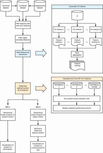
The flow chart in Figure 1 outlines the entire methodology for determining the similarity between playing positions (Aim 1) and players (Aim 2) in terms of displacement and technical performance indicators. The analysis was repeated three times to include three different datasets: 1) match displacement features only, collected from microtechnology devices; 2) technical performance indicators only, collected from notational analysis; 3) combined dataset including both match displacement and technical performance indicators. For the purposes of this study, playing positions at the most residual level were considered as 8 standard positions (i.e., fullback, wings, centres, halves, hooker, props, second-rows, loose forward). Left and right positional variations (e.g., left wing and right wing) were not considered and were treated as the same position. This is because players can swap left and right sides, even within a match, which makes assigning a position label that represents the whole match problematic. Whereas players are much less likely to swap positions entirely. All analyses outlined below were completed in R (version 4.0.2).

Figure 1. Schematic diagram of the feature selection and hierarchical clustering analysis methodology used.

Match displacement data were from a league-wide project (i.e., “Project SL-Catapult”). Within the project, all SL clubs use the same microtechnology devices (Optimeye S5, Catapult Sports, Melbourne, Australia; Firmware version = 7.17) and software (Openfield™, Catapult Sports, Melbourne, Australia; Software version = 3.1.0) for downloading raw data and subsequent uploading to Catapult servers. The research team then accessed 10-Hz sensor data files for further data processing and filtering. These data and filtering processes were the same as those used by Dalton-Barron, Palczewska et al. (2020), resulting in the identical displacement data. Included are 7617 observations collected from 11 SL teams and 366 senior male professional SL players. Matches included are from the 2018 and 2019 SL seasons; the Middle 8s phase of the 2018 season was excluded since it included Championship teams. This dataset also includes 35 discretised displacement metrics stratified by phases-of-play (i.e. attack, defence and transition phases), and are both absolute (i.e. total distance, high-speed running [HSR] distance, sprint distance) and relative to playing time (i.e. average speed, HSR distance per minute, sprint distance per minute, and absolute acceleration [Delaney et al., 2016]). Each match observation’s associated technical match performance indicators were then extracted from Opta (Stats Perform, London, UK) Superscout files. Initially, 558 technical features were extracted that included both actions (e.g., pass) and action outcomes (e.g., pass completed). Upon consultation with two expert rugby league coaches, these were then reduced to 41 key technical features, which were then expressed both in absolute terms and relative to playing duration, totalling 82 features. Both coaches have international coaching experience and have over 15- and 30-years’ coaching professionally within the SL and NRL, respectively.

Feature ranking using ensemble feature selection

Firstly, taking an initial dataset, features were filtered if they displayed near zero variance using the “nearZeroVar” function from the Caret package (Kuhn, 2008; frequency cut off ratio = 100/1, unique values = 10%). Near zero variance features have few unique values and occur infrequently in the data, and as such likely contain little valuable predictive information (Kuhn, 2008). The frequency cut off ratio and proportion of unique values are two frequently used indicators of near zero variance. Features were also filtered if they were highly correlated with another variable (r > 0.8). Removing highly correlated variables prior to feature selection is a common process to reduce model complexity (Andersen & Bro, 2010), without altering the feature space such as in PCA (Graham, 2003). This resulted in 39 features removed from the technical dataset and 15 features removed from the displacement dataset. For descriptive data including median and quartile ranges for each position and dataset see Supplementary File 1.

Features were then ranked according to their importance for classifying playing position at the most residual level (i.e. fullback, wing, centre, halves, hooker, loose forward, second row, prop) using an ensemble of feature selection techniques including filter, wrapper, and embedded methods. The objective of feature selection is to select an optimal subset of the original features within a dataset, such that the end model employed on the data contains a reduced set of features that maintain or even improve predictive performance. For a comprehensive review of feature selection and available methods see, Guyon and Elisseef (2003). The details of each feature selection technique used in this study, as well as their implementation in R, are outlined in Table 1. Multiple feature selection techniques were used to compensate for potential biases encountered using a single technique (Prati, 2012). Each technique provided its own base feature ranking according to each technique’s definition of importance. After which all base rankings were aggregated based on the order of each base ranking via the “Borda Count” voting system (Prati, 2012). The Borda count of a feature is its mean position in all base rankings, that is:

$\mathrm{B}\mathrm{o}\mathrm{r}\mathrm{d}\mathrm{a}\left(\mathrm{i}\right)={\sum }_{j=1}^{\mathrm{n}}{\pi }_{\mathrm{j}}\left({\mathrm{f}}_{\mathrm{i}}\right)$

Table 1. Feature selection approaches taken and their implementation.

Method	R implementation	Type	Data pre-process	Reference
Chi2	FSelector	Filter	Mean centre and standardize	Cheng et al., 2012
Information gain	FSelector	Filter	NA	Cheng et al., 2012
LDA RFE	Caret	Wrapper	Mean centre and standardize	Kuhn, 2008
Boruta	Boruta	Wrapper	NA	Kursa & Rudnicki, 2010
GBM	xgboost	Embedded	NA	Chen et al., 2018
Random forest	randomForest	Embedded	NA	Liaw & Wierner, 2007

LDA = Linear discriminant analysis; RFE = Recursive feature elimination; GBM = Gradient boosting machines.

where ${\pi }_j\left({\mathbf{f}}_{\mathrm{i}}\right)$ is the rank of feature ${\mathbf{f}}_i$ in the ranking ${\pi }_j$.

Determining optimal number of important features

To determine the optimal number of important features for the subsequent clustering analysis (i.e., the minimum number of important variables that still hold high predictive performance), 1 to k features were recursively inputted as predictors in a random forest. The randomForest function from the randomForest package was used. 500 trees were inputted and the number of features used at each split was calculated as the square root of the total number of inputted features. Each random forest model was then cross-validated to gain the area-under-curve (AUC) statistic, whereby data were split by 70% training and 30% testing. Since the AUC requires a binary classification, multiple receiver-operator characteristic (ROC) curves were calculated for the classification of each position using the pROC package. The AUC was extracted from each ROC curve and the median AUC across all classifications was taken to gain overall model predictive performance. Each random forest was run 100 times to gain a stable AUC statistic. The AUCs from each dataset were then visually inspected and a judgement was made on the number of features to retain for subsequent analyses, based on the point at which the AUC plateaus. Subsequently, the top 12 technical features, the top 11 displacement features, and the top 24 combined features were retained for further analysis (Figure 2).

Figure 2. Results of the random forest for classifying position within each dataset, using k most important features. The dashed vertical line represents the chosen number of features to retain for subsequent analysis. Sub-plot A uses technical features only; B uses displacement features only; C uses technical and displacement features.

Hierarchical cluster analysis

Two hierarchical cluster analyses were then applied to each of the three filtered datasets. The first hierarchical cluster was conducted at the positional level (Aim 1) and the second at the player level (Aim 2). For the positional level analysis, data were grouped by position and the mean taken for each feature. Data were then normalised (mean centred and scaled to unit variance) since there was a variety of features calculated in different units. Ward’s method of agglomerative hierarchical clustering was used to logically cluster positions (Ward, 1963), using a squared Euclidean distance matrix. Briefly, Ward’s method starts with each observation, then finds pairs of clusters with the smallest within-cluster error sum-of-squares increase; hence the method is sometimes termed the “minimum variance method”. The “ward.D2” implementation in R was used here (Murtagh & Legendre, 2014). The results were then visualised on a dendrogram.

For the player level analysis, players were first labelled according to their most frequently played starting position. Starting positions for each player were provided by Opta. Data were then grouped by their associated player ID and the mean taken for each feature, at which point the data were then also normalised. Observations were filtered if the player did not play at least five matches in their respective position. The same cluster procedure as the positional level was applied at the player level. However, since there were so many observations, PCA was also applied on the same dataset to visualise the results in a 2-dimensional space. PCA is an eigenvector-based method and is one of the most common techniques for dimension reduction (Ringnér, 2008). Taking a high-dimensional dataset, it is possible to create a linear set of orthogonalized composite variables, termed the principal components with minimal loss of information. The original data can then be projected onto the first two principal components for visualisation. Ward’s method of agglomerative hierarchical clustering is complementary to PCA since it utilises the same multivariate Euclidean space to find its clusters. As such the identified clusters are likely to be found in high density areas of PCA ordination (Murtagh & Legendre, 2014). Two principal component plots were created for each dataset, both are projections of the original data in eigenspace, with each point representing a player and their colour representing either their position or their cluster membership. Data ellipses representing 90% of the data were also drawn in each principal component plot around each class (either position or cluster). Lastly, the NbClust function was also applied to find the optimal number of clusters within each dataset, which implements 30 commonly used indices and suggests the best clustering scheme according to the majority rule. For a full conceptual and mathematical outline of the function and its indices, see, Charrad et al. (2014).

Results

For descriptive data of each feature used in each of the datasets see Supplementary File 1. Figure 2 shows the AUCs extracted from the random forests built for classifying position, as a function of the number of inputted important features. The median AUCs at the chosen number of features (i.e. the dashed vertical line) were 0.77, 0.84, 0.82 for the technical, displacement, and combined datasets respectively. Table 2 shows the top 10 extracted features from each dataset. For a full list of aggregated feature rankings and descriptions see Supplementary File 2.

Table 2. Top 10 features selected for each dataset determined through ensemble feature selection.

Ranking	Technical	Displacement	Combined
1	Total tackles/min	Total distance – Attack	Total tackles/min
2	Total tackles	HSR distance – Attack	Total distance – Attack
3	Caught full	Absolute acceleration – Defence	Total tackles
4	Defensive catch – Success	Average speed – Defence	HSR distance – Attack
5	Kick outcome – Touch	Average speed – Attack	Average speed – Attack
6	Kick outcome – Collected bounced	HSR distance – Transition	Average speed – Defence
7	Total carries	Total distance – Defence	Absolute acceleration – Defence
8	Quick PTB/min	Total distance – Transition *	Caught full
9	Carry outcome – Offensive miss	Absolute acceleration – Transition *	HSR distance – Transition
10	Quick PTB	Sprint distance – BIP	Total distance – Defence

* = Feature ranking is tied; HSR = High-speed running; PTB = Play-the-ball.

Positional clustering

The results of the hierarchical cluster analysis at the positional level are presented in Figure 3. Up to seven possible clusters may be extracted from each dendrogram through “cutting” the dendrogram at different thresholds. However, for the technical dataset there appears to be three clear clusters which include: Technical cluster 1 (Tech^C1) = Props, loose forwards, second-rows and hooker; Tech^C2 = Halves; Tech^C3 = Wings, centres and fullback. For displacement, four clusters are noted which include: Displacement cluster 1 (Disp^C1) = Props, loose forwards and hooker; Disp^C2 = Second-rows and halves; Disp^C3 = Fullback; Disp^C4 = Wings and centres. For the combined dataset, there are arguably three clusters which include: Combined cluster 1 (Comb^C1) = Props, loose forward, hooker and second-rows; Comb^C2 = Halves and fullback; Comb^C3 = Wings and centres.

Figure 3. Series of dendrograms showing the results of the hierarchical cluster analysis on the positional means. Sub-plot a uses technical features only; b uses displacement features only; c uses technical and displacement features.

Player clustering

Figure 4 shows the results of the hierarchical cluster analysis at the player level and includes a series of principal component plots. For the full results of the PCA applied to each dataset, including the eigenvalues, eigenvectors, and percent variance explained by each principal component see Supplementary Files 4A, 4B, and 4C.

Figure 4. Series of PC-plots showing the results of the hierarchical cluster analysis on the player means. Each point represents the player’s centroid and the colour represents either their correct position (as in A1, B1, and C1) or their cluster membership (as in A2, B2, and C2). The ellipses are drawn from the bivariate normal distribution and represent 90% of the data for its class. Sub-plots A1 and A2 are technical features; B1 and B2 are displacement features; C1 and C2 are technical and displacement features.

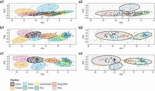
From the NbClust function applied to each dataset, three clusters were found in the technical dataset which consisted of: Technical cluster 1 (Tech^C1) = Props (proportion of total players in position assigned to cluster = 100%), loose forwards (100%), second-rows (91%) and hookers (100%); Tech^C2 = Halves (89%); Tech^C3 = Wings (100%), centres (85%) and fullbacks (100%; Table 3).

Table 3. Results of our hierarchical cluster analysis for each dataset. The values show the count of players assigned to each cluster for each position.

Positions	Technical			Displacement				Combined
	1	2	3	1	2	3	4	1	2	3
Loose forwards	27	0	0	0	27	0	0	27	0	0
Centres	6	0	35	1	0	40	0	0	0	41
Fullbacks	0	0	17	0	0	0	17	0	0	17
Halves	1	33	3	36	0	1	0	1	35	1
Hookers	21	0	0	0	21	0	0	21	0	0
Props	58	0	0	0	58	0	0	58	0	0
Second rows	45	0	4	43	6	1	0	49	0	0
Wings	0	0	34	0	0	33	1	0	0	34

Four clusters were identified for the displacement dataset: Displacement cluster 1 (Disp^C1) = Props (100%), loose forwards (100%) and hookers (100%); Disp^C2 = Second-rows (86%) and halves (97%); Disp^C3 = Fullbacks (100%); Disp^C4 = Wings (97%) and centres (98%; Table 3).

Finally, three clusters were found for the combined dataset: Combined cluster 1 (Comb^C1) = Props (100%), loose forwards (100%), second-rows (100%) and hookers (100%); Comb^C2 = Halves (95%); Comb^C3 = Wings (100%), centres (100%) and fullbacks (100%; Table 3).

Table 3 also shows the count of players within each position and their associated cluster membership. Supplementary Files 5A, 5B, and 5C show the same principal component plots as in Figure 4 for player clusters using all possible clusters from 2 to 7.

Discussion

The primary aim of this study was to determine the similarity between positions in professional rugby league by using analyses that include both physical and technical characteristics. This study implemented a novel framework which firstly used supervised feature selection to identify important technical and displacement features for classifying position. After which positions were clustered using those important features as inputs into three separate hierarchical cluster analyses, which included technical only features, displacement features, and a combined dataset. The dendrograms and principal component plots produced from the analysis provide a visual insight into the similarity between playing positions and players, respectively. Using these visuals, practitioners and researchers may choose the number of clusters to extract from each dataset as required. For example, if 4 clusters are required the dendrograms in the positional clusters can be cut at the desired level and the resulting positional groups can be used. The use of a league-wide sample over two competitive seasons also allows researchers and practitioners greater confidence in the generalisability of the presented results.

Determining logical positional groups using position labels

At the positional level, there appears to be common clusters across the three datasets (Figure 3). Firstly, wings and centres are consistently clustered across displacement, technical, and combined datasets, which is expected given their similarities in attacking and defensive roles (Sirotic et al., 2011). Fullbacks are often also grouped with centres and wings to form the “outside backs” positional group (e.g., Cummins & Orr, 2015; Twist et al., 2014; Waldron et al., 2011). This is reflected in the technical only dataset (Tech^C3), but not in the displacement dataset where fullbacks form their own cluster (Disp^C3) or the combined dataset where they are more similar to halves (Comb^C2). The latter is somewhat surprising given their distinct positional roles, particularly in defence where a fullback’s main responsibilities involve covering the goal line from kicks and breaks in the defensive line. Although some authors have previously included both halves and fullbacks in a broader “adjustables” group, along with hookers (Cummins et al., 2016; Gabbett et al., 2011).

Another common grouping across all three datasets includes props, loose forwards, and hookers (Tech^C1, Disp^C1, Comb^C1). The emergence of this cluster could be due to a number of reasons, however the increased tackling involvements these positions experience during match play compared to other positions is notable (Supplementary File 1; Naughton et al., 2020). Also, these positions tend to have less carries, catches, kicks, kick returns, and quick play-the-balls (Supplementary File 1; Johnston et al., 2014), all of which were deemed important for predicting positions for technical and combined datasets within the ensemble feature selection step (Table 2). It could be argued that the reduction in carries could be due to these positions being typically interchanged, and that by including carries per minute may resolve this. However, this was accounted for in the initial filtering step of the current framework and carries-per-minute was removed since it was highly correlated with total carries (r > 0.8). Given the known interplay between contact involvements and displacement (Johnston et al., 2019), it also not surprising that these positions cluster together when looking at solely displacement (Disp^C1).

Props and loose forwards are often grouped together in research as “middles” or “hit up forwards” (e.g., Scott et al., 2017). However, it is somewhat surprising that hookers are more related to this group than halves, since in attack the three positions work together to organise the area around the ruck and the attacking structure in general (Sirotic et al., 2011). Instead, halves are a unique position in the technical dataset (Tech^C2), which is likely due to their kicking responsibilities which appear as important variables (Table 2). Interestingly, for displacement, halves are much more related to the second-row position (Disp^C2) and both are somewhat similar to the wings and centres (Figure 3(b)). Again, this could be explained by a number of different reasons but is likely related to their similarities in spatial occupancy. Although second-rows are commonly labelled as “forwards” they do operate in wider channels to provide attacking and defensive support. This increased space allows second-rows to accumulate more high-speed running than props, loose forwards, and hookers (Supplementary File 1), which may help to explain their dissimilarity. For example, the props (n = 2), hooker and loose forward are typically the “middle” four, and the second-row, half-back, centre and wing are the “edge” four on each side.

Determining logical positional groups using player labels

Given the large between-player (i.e. within-position) variability found previously for the same displacement variables used here (Dalton-Barron, Palczewska et al., 2020), different clusters were expected to form at the player level analysis. However, the identified positional clusters are exactly the same as those identified at the positional level. Aside from the combined dataset where fullbacks join with centres and wings in the player level analysis instead of halves. This study also found very good separation between positions (Figure 4 a1, b1, c1), and players tend to cluster very well with their positional counterparts (Figure 4 a2, b2, c2) which can be seen visually in the principal component plots (Figure 4). Practically, this means there is more dissimilarity between-position centroids than there exists within-positions for both technical and displacement datasets and suggests that data may be aggregated at the positional level. That being said, the methodology used to identify similarity between players may be used in other applications. For example, to help guide team selection; if a player is injured coaches may wish to choose a player who displays similar technical qualities. The dendrograms and principal component plots may act as a tool to visualise highly complex data, whilst supplementing the numerical data.

Whilst feature selection has been implemented previously in sport as a pre-process step (Bunker & Thabtah, 2019; Wundersitz et al., 2015), to the authors’ knowledge this is the first study to use an ensemble of techniques, which includes expert-domain led feature selection, in team sports. Importantly, there is variation in the taxonomy of the identified important features (Table 2). This means the variables inputted in the subsequent hierarchical cluster analyses represents a holistic overview of match play instead of focusing on solely a single aspect, such as only attacking play. For the technical dataset, the most important predictors of position are related to forward attacking play (e.g., tackle busts), defensive play (e.g., total tackles), and kicking and catching qualities. Whereas for the displacement dataset, the most important features identified relate to attacking, defensive, and transition running. They also include cumulative metrics (e.g., total distance, HSR distance, sprint distance) and metrics relative to playing time (e.g., average speed, average acceleration). This also outlines an important limitation of this study which is the reliance on discrete data for both technical and displacement data. That is not to say the current data are not useful; rather the inclusion of spatial and temporal properties in the data may yield new insights into the clustering of positions. Nonetheless, the variables included in this study are some of the most commonly used in rugby league for studies that use technical (e.g., Parmar et al., 2018; Wedding et al., 2020; Woods et al., 2017) or displacement features (e.g., Delaney et al., 2016; Kempton & Coutts, 2016; Sirotic et al., 2011).

Conclusion

In conclusion, the positional clusters identified can be used to standardise positional groups in future research investigating either technical, displacement, or combined features in senior men’s rugby league. Importantly, whilst it appears that three clusters emerge from the technical and combined datasets, and four clusters from the displacement dataset, practitioners and researchers may choose the number of clusters to extract from each dataset as required. For example, if 4 clusters are needed the dendrograms can be cut at the desired level and the resulting positional groups can be used. Whilst within-position (i.e. between-player) variability did exist in all datasets, the separation between classes was still large enough to clearly demarcate the clusters in these data. However, performing cluster analyses at the player level may still be warranted if practitioners were interested in the similarity between individual players in their team. Ensemble feature selection may also be used and generalised to other problems in research or practice, where the objective is to identify important features without changing their original semantic value.

Disclosure statement

No potential conflict of interest was reported by the author(s).

Supplementary material

Supplemental data for this article can be accessed online https://doi.org/10.1080/02640414.2022.2100781.

Additional information

Funding

The author(s) reported there is no funding associated with the work featured in this article.

References

- Abdi, H., & Williams, L. J. (2010). Principal component analysis. Wiley Interdisciplinary Reviews: Computational Statistics, 2(4), 433–459. Wiley. https://doi.org/10.1002/wics.101
- Andersen, C. M., & Bro, R. (2010). Variable selection in regression-a tutorial. Journal of Chemometrics, 24(11–12), 728–737. https://doi.org/10.1002/cem.1360
- Austin, D., Gabbett, T., & Jenkins, D. G. (2011). Repeated high-intensity exercise in a professional rugby league. Journal of Strength and Conditioning Research, 25(7), 1898–1904. https://doi.org/10.1519/JSC.0b013e3181e83a5b
- Austin, D., & Kelly, S. J. (2014). Professional rugby league positional match-play analysis through the use of global positioning system. Journal of Strength and Conditioning Research, 28(1), 187–193. https://doi.org/10.1519/JSC.0b013e318295d324
- Bunker, R. P., & Thabtah, F. (2019). A machine learning framework for sport result prediction. Applied Computing and Informatics, 15(1), 27–33. https://doi.org/10.1016/j.aci.2017.09.005
- Charrad, M., Ghazzali, N., Boiteau, V., & Niknafs, A. (2014). NbClust: An R package for determining the relevant number of clusters in a data set. Journal of Statistical Software, 61(6), 1–36. https://doi.org/10.18637/jss.v061.i06
- Chen, T., He, T., Benesty, M., Khotilovich, V., & Tang, Y. (2018) xgboost: Extreme Gradient Boosting. R Package Version 1.6.0.1. 2–5. https://cran.r-project.org/package=xgboost
- Cheng, T., Wang, Y., & Bryant, S. H. (2012). FSelector: A Ruby gem for feature selection. Bioinformatics, 28(21), 2851–2852. https://doi.org/10.1093/bioinformatics/bts528
- Cummins, C., & Orr, R. (2015). Analysis of physical collisions in elite national rugby league match play. International Journal of Sports Physiology and Performance, 10(6), 732–739. https://doi.org/10.1123/ijspp.2014-0541
- Cummins, C., Gray, A., Shorter, K., Halaki, M., & Orr, R. (2016). Energetic and metabolic power demands of national rugby league match-play. International Journal of Sports Medicine, 37(7), 552–558. https://doi.org/10.1055/s-0042-101795
- Dalton-Barron, N., Palczewska, A., McLaren, S. J., Rennie, G., Beggs, C., Jones, B., & Roe, G. (2020). A league-wide investigation into variability of rugby league match running from 322 Super League games. Science and Medicine in Football, 5(1), 1–25. https://doi.org/10.1080/24733938.2020.1844907
- Dalton-Barron, N., Whitehead, S., Roe, G., Cummins, C., Beggs, C., & Jones, B. (2020). Time to embrace the complexity when analysing GPS data? A systematic review of contextual factors on match running in rugby league. Journal of Sports Sciences, 38(10), 1161–1180. https://doi.org/10.1080/02640414.2020.1745446
- Delaney, J. A., Duthie, G. M., Thornton, H. R., Scott, T. J., Gay, D., & Dascombe, B. J. (2016). Acceleration-based running intensities of professional rugby league match play. International Journal of Sports Physiology and Performance, 11(6), 802–809. https://doi.org/10.1123/ijspp.2015-0424
- Gabbett, T., King, T., & Jenkins, D. G. (2008). Applied physiology of rugby league. Sports Medicine, 38(2), 119–138. https://doi.org/10.2165/00007256-200838020-00003
- Gabbett, T., Jenkins, D. G., & Abernethy, B. (2010). Physical collisions and injury during professional rugby league skills training. Journal of Science and Medicine in Sport, 13(6), 578–583. https://doi.org/10.1016/j.jsams.2010.03.007
- Gabbett, T., Jenkins, D. G., & Abernethy, B. (2011). Physical collisions and injury in professional rugby league match-play. Journal of Science and Medicine in Sport, 14(3), 210–215. https://doi.org/10.1016/j.jsams.2011.01.002
- Gabbett, T., Jenkins, D. G., & Abernethy, B. (2012). Physical demands of professional rugby league training and competition using microtechnology. Journal of Science and Medicine in Sport, 15(1), 80–86. https://doi.org/10.1016/j.jsams.2011.07.004
- Glassbrook, D. J., Doyle, T. L. A., Alderson, J. A., & Fuller, J. T. (2019). The demands of professional rugby league match-play: A meta-analysis. Sports Medicine - Open, 5(1), 24. https://doi.org/10.1186/s40798-019-0197-9
- Graham, M. H. (2003). Confronting multicollinearity in ecological multiple regression. Ecology, 84(11), 2809–2815. https://doi.org/10.1890/02-3114
- Guyon, I., & Elisseef, A. (2003). An introduction to variable and feature selection. Journal of Machine Learning Research, 3(March) , 1157–1182. https://doi.org/10.5555/944919.944968
- Johnston, R. D., Gabbett, T., & Jenkins, D. G. (2014). Applied sport science of rugby league. Sports Medicine, 44(8), 1087–1100. https://doi.org/10.1007/s40279-014-0190-x
- Johnston, R. D., Weaving, D., Hulin, B. T., Till, K., Jones, B., & Duthie, G. (2019). Peak movement and collision demands of professional rugby league competition. Journal of Sports Sciences, 37(18), 2144–2151. https://doi.org/10.1080/02640414.2019.1622882
- Kempton, T., & Coutts, A. J. (2016). Factors affecting exercise intensity in professional rugby league match-play. Journal of Science and Medicine in Sport, 19(6), 504–508. https://doi.org/10.1016/j.jsams.2015.06.008
- Kempton, T., Sirotic, A. C., & Coutts, A. J. (2017). A comparison of physical and technical performance profiles between successful and less-successful professional rugby league teams. International Journal of Sports Physiology and Performance, 12(4), 520–526. https://doi.org/10.1123/ijspp.2016-0003
- King, T., Jenkins, D. G., & Gabbett, T. (2009). A time-motion analysis of professional rugby league match-play. Journal of Sports Sciences, 27(3), 213–219. https://doi.org/10.1080/02640410802538168
- Kuhn, M. (2008). Building predictive models in r using the caret package. Journal of Statistical Software, 28(5), 1–26. https://doi.org/10.18637/jss.v028.i05
- Kursa, M. B., & Rudnicki, W. R. (2010). Feature selection with the boruta package. Journal of Statistical Software, 36(11), 1–13. https://doi.org/10.18637/jss.v036.i11
- Liaw, A., & Wierner, M. (2002). Classification and Regression by randomForest. R News, 2(3), 18–22. https://www.r-project.org/doc/Rnews/Rnews_2002-3.pdf
- Murray, N. B., Gabbett, T., & Chamari, K. (2014). Effect of different between-match recovery times on the activity profiles and injury rates of national rugby league players. Journal of Strength and Conditioning Research, 28(12), 3476–3483. https://doi.org/10.1519/JSC.0000000000000603
- Murtagh, F., & Legendre, P. (2014). Ward’s Hierarchical agglomerative clustering method: Which algorithms implement ward’s criterion? Journal of Classification, 31(3), 274–295. https://doi.org/10.1007/s00357-014-9161-z
- Naughton, M., Jones, B., Hendricks, S., King, D., Murphy, A., & Cummins, C. (2020). Quantifying the collision dose in rugby league: A systematic review, meta-analysis, and critical analysis. Sports Medicine - Open, 6(1), 6. https://doi.org/10.1186/s40798-019-0233-9
- Oxendale, C. L., Twist, C., Daniels, M., & Highton, J. (2016). The relationship between match-play characteristics of elite rugby league and indirect markers of muscle damage. International Journal of Sports Physiology and Performance, 11(4), 515–521. https://doi.org/10.1123/ijspp.2015-0406
- Parmar, N., James, N., Hearne, G., & Jones, B. (2018). Using principal component analysis to develop performance indicators in professional rugby league. International Journal of Performance Analysis in Sport 18(6), 938–949. https://doi.org/10.1080/24748668.2018.1528525
- Polglaze, T., Dawson, B., & Peeling, P. (2016). Gold standard or fool’s gold? The efficacy of displacement variables as indicators of energy expenditure in team sports. Sports Medicine, 46(5), 657–670. https://doi.org/10.1007/s40279-015-0449-x
- Prati, R. C. (2012). Combining feature ranking algorithms through rank aggregation. Proceedings of the international joint conference on neural networks, Cmcc. https://doi.org/10.1109/IJCNN.2012.6252467
- Quarrie, K. L., Hopkins, W. G., Anthony, M. J., & Gill, N. D. (2013). Positional demands of international rugby union: Evaluation of player actions and movements. Journal of Science and Medicine in Sport, 16(4), 353–359. https://doi.org/10.1016/j.jsams.2012.08.005
- Remeseiro, B., & Bolon-Canedo, V. (2019). A review of feature selection methods in medical applications. Computers in Biology and Medicine, 112(July), 103375. https://doi.org/10.1016/j.compbiomed.2019.103375
- Rennie, G., Dalton-Barron, N., McLaren, S. J., Weaving, D., Hunwicks, R., Barnes, C., Emmonds, S., Frost, B., & Jones, B. (2020). Locomotor and collision characteristics by phases of play during the 2017 rugby league world cup. Science and Medicine in Football, 4(3), 225–232. https://doi.org/10.1080/24733938.2019.1694167
- Ringnér, M. (2008). What is principal component analysis? Nature Biotechnology, 26(3), 303–304. https://doi.org/10.1038/nbt0308-303
- Saeys, Y., Inza, I., & Larrañaga, P. (2007). A review of feature selection techniques in bioinformatics. Bioinformatics, 23(19), 2507–2517. https://doi.org/10.1093/bioinformatics/btm344
- Scott, T. J., Thornton, H. R., Scott, M. T. U., Dascombe, B. J., & Duthie, G. M. (2018). Differences between relative and absolute speed and metabolic thresholds in rugby league. International Journal of Sports Physiology and Performance, 13(3), 298–304. https://doi.org/10.1123/ijspp.2016-0645
- Sirotic, A. C., Knowles, H., Catterick, C., & Coutts, A. J. (2011). Positional match demands of professional rugby league competition. Journal of Strength and Conditioning Research, 25(11), 3076–3087. https://doi.org/10.1519/JSC.0b013e318212dad6
- Twist, C., Highton, J., Waldron, M., Edwards, E., Austin, D., & Gabbett, T. (2014). Movement demands of elite rugby league players during Australian national rugby league and European super league matches. International Journal of Sports Physiology and Performance, 9(6), 925–930. https://doi.org/10.1123/ijspp.2013-0270
- Varley, M. C., Gabbett, T., & Aughey, R. J. (2014). Activity profiles of professional soccer, rugby league and Australian football match play. Journal of Sports Sciences, 32(20), 1858–1866. https://doi.org/10.1080/02640414.2013.823227
- Waldron, M., Twist, C., Highton, J., Worsfold, P., & Daniels, M. (2011). Movement and physiological match demands of elite rugby league using portable global positioning systems. Journal of Sports Sciences, 29(11), 1223–1230. https://doi.org/10.1080/02640414.2011.587445
- Ward, J. H. (1963). Hierarchical grouping to optimize an objective function. Journal of the American Statistical Association, 58(301), 236–244. https://doi.org/10.1080/01621459.1963.10500845
- Weaving, D., Jones, B., Ireton, M., Whitehead, S., Till, K., & Beggs, C. B. (2019). Overcoming the problem of multicollinearity in sports performance data: A novel application of partial least squares correlation analysis. PloS One, 14(2), e0211776. https://doi.org/10.1371/journal.pone.0211776
- Weaving, D., Beggs, C., Dalton-Barron, N., Jones, B., & Abt, G. (2019). Visualizing the complexity of the athlete-monitoring cycle through principal-component analysis. International Journal of Sports Physiology and Performance, 14(August), 1304–1310. https://doi.org/10.1123/ijspp.2019-0045
- Wedding, C., Woods, C. T., Sinclair, W. H., Gomez, M. A., & Leicht, A. S. (2020). Examining the evolution and classification of player position using performance indicators in the national rugby league during the 2015–2019 seasons. Journal of Science and Medicine in Sport, 23(9), 891–896. https://doi.org/10.1016/j.jsams.2020.02.013
- Woods, C. T., Sinclair, W., & Robertson, S. (2017). Explaining match outcome and ladder position in the national rugby league using team performance indicators. Journal of Science and Medicine in Sport, 20(12), 1107–1111. https://doi.org/10.1016/j.jsams.2017.04.005
- Wundersitz, D. W. T., Josman, C., Gupta, R., Netto, K. J., Gastin, P. B., & Robertson, S. (2015). Classification of team sport activities using a single wearable tracking device. Journal of Biomechanics, 48(15), 3975–3981. https://doi.org/10.1016/j.jbiomech.2015.09.015