A remote temperature sensor for an ultrasound hyperthermia system using the acoustic signal derived from the heating signals

Abstract

We demonstrate a non-invasive technique, based on the modal frequency shift of a region insonified by a dual-beam ultrasound (US) transducer (region of interest, ROI), to remotely assess the temperature of the region in a tissue-mimicking object. The application is in ultrasound hyperthermia systems for controlled maintenance of tumour temperature during chemotherapy. Towards this, we have characterised the variation of the storage modulus with the temperature of two tissue-mimicking visco-elastic materials. Due to this variation in tissue storage modulus (and viscosity), we have observed a shift in the resonant modes of the ROI, vibrated remotely with a dual-beam focussed ultrasound transducer. A modal analysis of the vibrating ROI is done to identify the modes captured by the detector. A variation in this modal frequency with temperature is computed and matches reasonably well with the experimental measurements. Through this, we demonstrate that an ultrasound hyperthermia system can have a remote temperature sensor without using an additional imaging modality.

Keywords:

• Hyperthermia
• modal analysis
• remote monitoring
• phantoms
• temperature dependence

Introduction

Hyperthermia, a treatment for cancer in which a selected region of the body is maintained at an elevated range of temperatures (e.g. 5 °C above the ambient temperature of 37 °C), is gaining popularity. This is due to its advantage of enhancing the efficacy of other popular treatment protocols such as radiation therapy and chemotherapy in destroying malignant cells. Studies have also shown that with selective heating alone, a tumour can be destroyed or incapacitated (because heat destroys the cell structure and damages the protein within [1]), leaving the surrounding normal tissue unharmed [2]. However, the greatest benefit of hyperthermia in cancer therapy is its contribution to the effectiveness of other treatment modalities such as radiation- and chemotherapies [2,3]. In addition, hyperthermia can also boost the action of certain anticancer drugs in patients. Several clinical trials have been conducted to examine the effect of hyperthermia when combined with radiation therapy and/or chemotherapy. These studies are focussed on the treatment of different types of cancer including sarcoma, melanoma and cancers of the head and neck, brain, lung, oesophagus, breast, bladder, rectum, liver, appendix, cervix and peritoneal lining (mesothelioma) [2–7]. Many of these researchers report a greater reduction in tumour size when hyperthermia is combined with other treatments [2,3,6,7].

A number of groups are working towards developing clinically feasible controlled ultrasound hyperthermia systems capable of maintaining large tumours at an elevated temperature uniformly [8,9]. A common feature of such systems is the high intensity focussed ultrasound (HIFU) transducers used for non-invasive delivery of heat locally [10–12]. However, HIFU has also been extensively used in other therapeutic applications, a notable example being the thermal ablation of tissue [13,14]. Also, significant are its applications in treating fibroids [15,16] and glaucoma [17] and enhancing the efficiency of drug delivery [18]. For hyperthermia per se, temperature monitoring plays a crucial role in the success of the treatment. Here, feedback control systems are designed wherein phased-array ultrasound systems capable of producing a spatially variable array of focal spots provide controlled heating [19]. The success of such a system depends crucially on the availability of accurate temperature measurements from the focal region of the HIFU in the tumour providing feedback to the control system. In early designs, the temperature measurement was done invasively with thermocouples stuck inside the object (i.e. the body). In addition to disturbing the ultrasound heating efficiency by providing an artificial scattering centre, the thermocouple, owing to a surgical procedure needed for insertion, raised doubts regarding the acceptability of the ultrasound hyperthermia system itself in the clinic. Therefore, non-invasive temperature measurement has been pursued to render a patient friendly controlled hyperthermia procedure. Accordingly, a number of methods have been tested, such as an ultrasound A-scan imager from which temperature-dependent parameters (speed of sound, elasticity and spacing of scatterers) are estimated, functional MRI images giving quantitative temperature information [20,21], microwave radiometry [22] and impedance tomography [23]. Both the temporal location of the back-scattered A-line pulse and the resonant frequencies it contains are linked to the temperature of the selected locations of heating [9]. In addition, van Dongen and Verweij reported non-invasive ultrasound thermometry [24] based on the variation of the non-linearity parameters (B/A) of sound propagation with temperature. Bing et al. [25] considered MR thermometry based on the accurate monitoring of proton resonant frequency (PRF) shift with temperature. However, all these methods suffer from a number of drawbacks. For example, maintaining continuous monitoring through an imaging ultrasound system is cumbersome. More importantly, the temperature assessment is not quite accurate both in value and in the spatial assignment to locations within the tumour. To make the entire hyperthermia system cost effective and simple, the need for a separate imaging modality within should be avoided. In this work, we suggest a procedure for non-invasive temperature measurement, making use of a measurement signal obtained by mixing two ultrasound heating signals. The main advantage of the present scheme, vis-à-vis the existing methods, is its ability to monitor temperature precisely at the region of heat application by deriving a proper transduction signal without the need for a separate system for doing so. Indeed, a pre-calibration exercise is required to make this measurement quantitatively accurate and, therefore, reliable. Since the heating and measurement are local, one is also able to retrieve the temperature distribution inside a larger object even before it has attained, or is on the way to attaining, a uniform temperature throughout. This is the motivation for introducing this new measurement technique (see also Discussion section).

We use two ultrasound transducers, synchronously driven by two RF sources of slightly differing frequencies, focussing sound waves on their focal regions and aligned to have a common intercept region, to deliver ultrasound energy for heating. In the intercepted volume, a difference frequency signal Δf (in our case of the order of 1 KHz) is also produced through mixing. This low frequency acoustic force sets the intercept region to mechanical vibration producing secondary acoustic waves, known in the literature as vibro-acoustic waves [26–28], which are detected at the object boundary. The vibration is confined to a local region around the intersecting ultrasound focal volume, denoted by the ROI, verified in reference [29] as a freely vibrating region. Therefore, the spectrum of the acoustic emission will reflect the visco-elastic properties, volume density of mass, size and shape of the vibrating ROI. Consequently, the resonant modes of the freely vibrating ROI can be read out from the measured vibro-acoustic spectrum. In fact, as shown in reference [29], the acoustic spectral peaks are the natural frequencies of vibration of the ROI, which means that these natural frequencies of vibration can be noninvasively measured. To measure the spectral peaks in the acoustic emission, the difference frequency Δf of the ultrasound is varied, and the acoustic wave reaching a detector on the surface of the body is measured, reflecting resonance-like peaks at certain Δf's. The dependence of the resonant modes on the elasticity of the material of the ROI, (apart from other parameters such as its size, shape and volume density of mass), provides us with a means to measure the “local” temperature by connecting the variation of natural frequencies to temperature through elasticity. It has been reported that for certain materials, this temperature co-efficient of resonance frequency is positive [30]. However, for materials that behave similar to human tissue (polymers, for instance), it is found to be negative [31]. Reference [30] considers elasticity to be the major contributor to such a shift in the resonant frequency. Since elasticity itself has a sensitive dependence on temperature, the resonant frequency is seen to vary with temperature with good sensitivity. The sensitivity improves as we consider the higher modes, as demonstrated in this study. We calibrate the shift in the resonant frequency against temperature and prove its usefulness for non-invasive temperature measurement. The method offers two notable advantages in comparison to earlier suggestions: (1) no additional paraphernalia is required (other than the ultrasound heating applicators) to arrive at the measurement signal, and (2) the signal corresponds exactly to the spot(s) where the heating signal is applied.

A summary of the rest of the paper is as follows: In Theory section, we elaborate the principle of the method. Here, we also give the equation describing the vibration of an elastic body subjected to sinusoidal forcing. In the latter part of this section, we discuss how the resonant frequencies of the vibrating region depend on temperature. First the dependence of the storage modulus on temperature is studied using a rheometer. Then, using this information, the variation of the resonant frequency with storage modulus is simulated, and its connection with temperature is established. Experimental verification section describes our experiments using PVA and agarose phantoms. For these phantoms, temperature is calibrated to measured resonant frequency shifts and compared with similar results from simulation studies reported in Theory section. The results are further discussed in the Results section. Discussion contains a comparative study of our technique with other existing ultrasound- and MRI-based thermometric techniques, followed by suggestions to extend it to heterogeneous materials and animal models. A major observation is the hysteresis in the experimentally measured storage modulus vs. temperature plots on temperature cycling, which should reveal itself also in the resonant frequency vs. temperature plots. Our concluding remarks are given in Conclusion section.

Theory

Acoustic radiation force in the ultrasonic focal volume

In arriving at the acoustic radiation force, we first compute the acoustic pressure distribution in the focal volume of the ultrasonic transducers. When the sound intensity is large, as in the focal region of the FUS, the nonlinearity of the material comes into play and should be accounted for when deriving the propagation equation. Thus, in our model, we have used an equation that is a simplified version of a more general nonlinear equation for acoustic wave propagation. This equation is given in references [32–34] (1) where δ and β are, respectively, the sound diffusivity and the coefficient of non-linearity of the material of the medium, v is the particle velocity, and L is the Lagrangian density function defined as L=ρ₀(v.v)/2-p²/2ρ₀c₀². When local effects can be ignored, Equation (1)(1) is approximated by the Westervelt equation: (2)

Under this approximation, it can model progressive quasi-plane waves with reasonable accuracy at distances more than a wavelength away from the acoustic source [35]. It can be seen that for acoustic waves in a stagnant medium, a progressive plane wave involves displacement of medium particles with a velocity v=p/ρ₀c₀ [36], which makes the Lagrangian term of Equation (1)(1) vanish. Strictly speaking, the equation obtained by Westervelt [37] is the loss-less version of Equation (2)(2) . We solve this equation, as is done in reference [38], by first writing it in an oblate-spheroidal co-ordinate system and then expanding it using the Fourier series. The resulting sets of coupled partial differential equations for the Fourier coefficients are solved using an implicit backward finite difference scheme. The numerical integration region ranges from 0 to π/2  on the θ axis and from the surface of the transducer (denoted as -σ_max in Figure 1 by Kamakura et al. [38]) to the observer position on the σ axis [refer Figure 1 in reference [38] for coordinates]. The θ axis was discretized, for facilitating a solution, using 450, 600 and 1000 grid-points in our work, and it was noticed that the solution is almost invariant to grid refinement beyond 450 points. With 600 grid-points, step-size Δθ is easily seen to be 0.15°, which was maintained uniformly across the entire range. In the axial direction (i.e. σ), the sampling was not uniform but decreased with σ. This was done to facilitate convergence of the algorithm used to invert the large matrices involved. For the simulations presented in this paper, the step-size was around 3.5*10^-3. Acoustic pressure was assumed to be axis-symmetric with respect to the φ- axis. The pressure (p₀) at the transducer’s surface was taken as 230 kPa to match the transducer used in the experiments. The inputs for solving the equation are specific to the transducers [39] and the phantoms used in the experiment. These parameters are given in Table 1.

Figure 1. Cross-sectional plot of the normalised pressure distribution of the transducer focal region. The cross-section contains the transducer axis x. Here, “a” and “d” are, respectively, the diameter and focal length of the transducer with the focal point located at the origin.

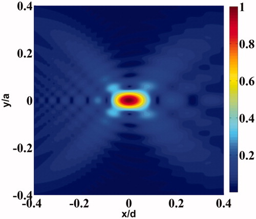
Table 1. Parameters for computing pressure distribution due to focused ultrasound transducer.

Frequency of excitation (f)	1.1 MHz
Radius of active surface	32 mm
Focal length	62.6 mm
Average velocity of sound in the object (c0)	1545 m/s (PVA) 1500 m/s (agarose)
Average mass density	1000 kg/m^3 (for both)
Non-linearity coefficient (β)	6.2(PVA) 3.5(agarose)
Sound attenuation coefficient(α=δω^2/2c0^3)	1 dB/cm (PVA) 0.1911 dB/m (agarose)
Pressure on the transducer surface (P0)	230 kPa
Frequency difference (Δf)	470–520 Hz (PVA) 1020–1070 Hz (agarose)

Figure 1 shows the cross-sectional pressure distribution due to one of the two identical focussed ultrasound transducers used in this work. The pressure distribution shown in this figure is axi-symmetric [38].

As mentioned in Introduction section, we have used two focussing ultrasonic transducers, both are identical in all respects, with one driven at a frequency of 1.1 MHz plus Δf/2 and the other at 1.1 MHz minus Δf/2, aligned in such a way that their focal volumes intersect at the thinnest region perpendicularly.

Beating of the acoustic waves takes place at the intercept volume (denoted again by ROI) giving a sinusoidal force which oscillates at a frequency Δf Hz, as well as one at approximately 2.2 MHz. We note that the force that is generated from acoustic intensity absorption and scattering depends on the square of the pressure [40]. The absorbed intensity of the ultrasonic pressure causes a temperature rise in the ROI. The force field generated at the difference frequency at a point x is given by reference [41] (3)

Here, F₀ depends on the squared pressure at the ROI induced by the two transducers, the acoustic absorption coefficient of the material in the ROI and the speed of sound.

We consider the force driving the material in the ROI and generating a secondary acoustic wave, which is detected at the boundary of the object. In the next section, the response of the object to the sinusoidal forcing is derived based on a force balance equation.

Natural frequencies of vibration of the ROI

The free vibration of the ROI depends, along with other material parameters such as the elastic modulus and volume density of the mass, on the projected shape and dimension of the freely vibrating region on the ultrasound beams. Therefore, it is important to ascertain the boundary ∂Ω of the ROI, in the interior of which the displacement amplitude is nonzero, to numerically compute the resonant (natural) frequencies of the body. To delineate ∂Ω, we solve the linear momentum balance equation for an infinite object driven by a sinusoidal forcing at the intersection volume of the focal regions of the two ultrasound transducers, given by Equation (3)(3) . This sinusoidal force distribution is observed to be approximately nonzero only over a small region including the intersection of the focal volumes of the ultrasound transducers. With this forcing, we set up the linear momentum balance equation, which is (4)

Here, u is the displacement vector field, σ is the Cauchy stress tensor, F₀(x) is the amplitude of the sinusoidal forcing at point x within the support region denoted by the indicator function, I_Ω, for the applied force. We have employed ANSYS^® to solve Equation (4)(4) for one full cycle of the sinusoidal forcing F(x,t)=F₀(x)cos(2πΔf₀t)IΩ and obtained a cycle of the vibration of the particles in the object, from which the amplitude of vibration is ascertained. Figure 2 shows schematically the orientation of the transducers during the experiments reported in Results section. The distribution of the force field due to a transducer, at an instant of time, is shown in Figure 3. The stress-free surface of the ROI, ∂Ω, is obtained by identifying the boundary nodes that separate the vibrating region from its non-vibrating complement. 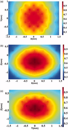For agarose and PVA, which are the materials used in the objects in the experiments reported here, we have set up Equation (4)(4) and arrived at ∂Ω. The amplitudes of vibration in three orthogonal planes passing through the centre of the object, here, agarose, are shown in Figures 4(a–c). We emphasise that the dynamics introduced are truly local and confined to within the ROI; therefore, the acoustic amplitude distribution generated is a function of the local mechanical (and acoustic) properties of the object.

Figure 2. Schematic diagram of the orientation of the two transducers (top view).

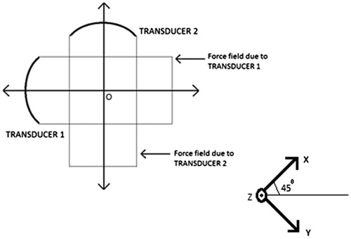
Figure 3. Contour plot of the force distribution (−6 dB) along the axial plane corresponding to Transducer 1 (refer to Figure 2). For Transducer 2, we get an identical plot, rotated clockwise by 90°. The colour bar shows normalised force distribution.

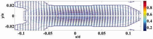
Figure 4. Axial cross-section of the maximum displacement in the focal region when driven by the difference frequency force obtained by “mixing” the radiation from the two transducers on the agarose phantom. (a) Simulated displacements in the Y–X plane of the agarose phantom. The colour bar shows normalised displacement magnitude. (b) Same as Figure 4(a), but in the Z–X plane. (c) Same as Figure 4(a), but in the Z–Y plane.

Having found the shape and volume of the ROI, we now proceed to compute its natural frequencies of mechanical vibration. We use a software package available in ANSYS^® to compute the resonant modes; however, a word about the principle used to compute the set of natural frequencies would perhaps be in order. Following a variational approach used to arrive at the governing Euler–Lagrange equations, an eigenvalue problem is set up for the unforced and undamped problem. The solution to this eigenvalue problem yields the natural frequencies [42]. Specifically, for a free body, i.e. with stress-free boundary conditions and the displacement vector u satisfying the elastic wave equation, the Lagrangian L=∫V(E_K-E_P)dV of the system is stationary. Here, E_K is the kinetic energy equal to (1/2)ρω²u_iu_i, and E_P is the potential energy given by (1/2)C_ijkl ∂_ju_i ∂_lu_k, where the usual sign convention of repeated indices is followed. Moreover, u_i, etc., are components of u that have harmonic time variations given by e^jωt, and ρ and C_ijkl are the volume density of mass and the elasticity tensor, respectively. The next step is to expand u_i in terms of a basis function set defined over V: u_i=u˜_i,λB_λ, λ=1,2….N. The principle δL=0 leads to the following computable equation, which is our symmetric eigenvalue problem: (5) where the mass matrix M is real, symmetric and positive definite, and the stiffness matrix Γ is real and symmetric. The elements of M and Γ are M_λi,λi^′=δ_i,i^′∫VB_λρB_λ′dV and , respectively. The concatenated column vector α is obtained by arranging all the coefficients u˜_i,λ of the displacement field u_i.

The major contribution of reference [43] to the development of an easily computable forward model that is applicable for any arbitrarily shaped (and sized) object is the introduction of a basis B_λ using monomials of the form B_λ=x^l(λ)y^m(λ)z^n(λ). The {Bλ}’s are not an orthogonal set; therefore, the matrix M is not diagonal with consequent loss of advantage in the inversion of Equation (5)(5) . In any case, since the orthonormal basis has to be chosen afresh for each problem depending on the shape of the object and the variation of ρ(r), we lose the usefulness of a generalised procedure for computing the matrix elements in closed form, valid for all arbitrary shapes. The basis with monomials allows us such a closed form with analytic expressions valid for any object, without destroying the symmetry and positive definiteness of M.

Assuming ∂Ω to be the free boundary of the ROI, we compute its resonant modes using ANSYS^®. The parameters to be input are (i) the geometry of the free boundary, (ii) the material parameters such as ρ, Young’s Modulus (Y) and Poisson’s ratio (0.495 in this present case) and (iii) the boundary conditions. A change in temperature in the ROI leads to a stiffness change therein, leading to a shift in the natural frequencies. With the present software, we are able to track these changes.

To complete the simulation of the dependence of Δf₀ (i.e. the resonant frequency) on temperature, we need the variation of the elastic properties of the object material with temperature. This input, we realise through the experimental measurement of storage modulus (G′) and loss modulus (G″), with temperature, using a rheometer, MCR102 Rheoplus, Anton Paar, for the agarose and PVA phantoms. Circular discs of thickness 0.6 mm and diameter 25 mm were used as samples. Prior to the temperature sweep (TS), the samples were subjected to an “amplitude sweep” (AS) wherein the shear-strain amplitude was varied within a preset range corresponding to first the maximum and then the minimum temperatures in the range. This was done to identify the amplitude at which the gel will yield (or be permanently damaged). During TS, the strain amplitude was maintained at a constant value within this “safe” amplitude range. Maintaining the selected constant strain amplitude, the temperature was varied slowly to cover the entire temperature range, planned previously. At each temperature, a wait of 5–7 min was needed to ensure the sample stabilised at the temperature of the plate that was measured in the instrument. These precautions were taken during both the heating and cooling parts of the temperature cycling. The measurements were repeated for five samples to generate data for arriving at the mean and standard deviation.

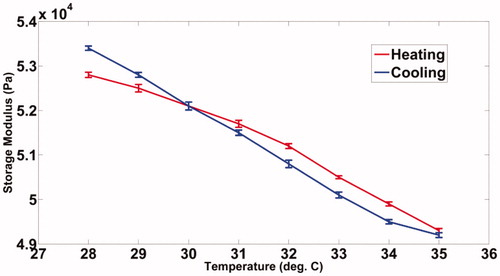
We have observed that the storage modulus of the PVA phantom drops from 6730 Pa to 6320 Pa, a typical range of shear modulus for normal soft tissue, when its temperature is increased from 34 °C to 41 °C as shown in Figure 5. Figure 6 also shows a decrease in the storage modulus for agarose, decreasing from 52 900 Pa to 49 300 Pa, a range chosen to mimic stiffer tumours, when the sample temperature is increased from 28 °C to 35 °C. A visco-elastic model that may reasonably approximate the behaviour of human tissue upon mechanical loading is the Kelvin–Voigt model [44,45]. Considering this model, it can be readily derived that the measured storage modulus (G′) of the phantoms is numerically equal to their shear modulus (G) [46]. The Young’s modulus required to compute the modes is three times the shear modulus for the present value of Poisson’s ratio of 0.495. The modal frequencies of the vibrating ROI at different temperatures are then computed using the modal analysis module available in ANSYS^®. The computed modal frequencies and their experimentally measured shift with temperature are further discussed in Results section.

Figure 5. Variation of the storage modulus of the PVA sample with temperature.

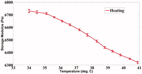
Figure 6. Variation of the storage modulus of the agarose sample with temperature.

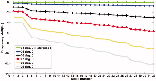
We have observed during the simulation study that the sensitivity of the resonant frequency shift with temperature continues to increase with the mode number, which is anticipated anyway. Keeping in mind this greater sensitivity, we have proceeded to target the higher modes in our experimental work. Figure 7 demonstrates this observation based on results obtained from simulation studies on the PVA phantom.

Figure 7. Plots showing the simulated resonant frequency shift vs. the mode number. It is evident that the temperature sensitivity of the modal frequency is higher when the mode number is higher.

Experimental verification

Experiments are performed on the tissue-mimicking phantoms of PVA and agarose to confirm our theoretical results for shift in the resonant frequencies with temperature.

Experiments with the PVA phantom

The phantoms used in this experiment are of the dimensions 40*40mm*70mm. The recipe for fabrication of PVA gels of different stiffness is given in references [47,48]. Similar details for fabrication of agarose are given in reference [49]. A resistance temperature detector (RTD), Pt100 of dimensions 1mm*1mm, is inserted inside the phantom while fabricating, allowing an independent measurement of the local temperature of the phantom targeted by the ultrasound focal region. The variation of the sample’s storage modulus, as measured with a rheometer, with temperature is shown in Figures 5 (PVA) and 6 (agarose). As mentioned earlier, these values have been used in our simulations using ANSYS^® to compute the resonant modes.

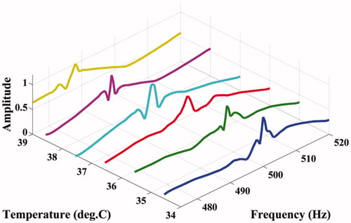
The experimental set-up to capture the resonant modes at various temperatures is shown in Figure 8. In this experiment, two H-101 high intensity focussed ultrasound (HIFU) transducers (Sonic Concepts, WA) are used to heat the ROI as well as to vibrate the same with the difference frequency Δf. We have designed a PID controller, the details of which conform to standard textbook material, to maintain the ROI at a particular temperature in the range of interest. A PC-based, micro-positioner-controlled three-axis translation stage (Holmarc Opto-Mechatronics Pvt. Ltd., Kerala, India) is used to adjust the orientation of the phantom so that, on the one hand, the RTD element inside the phantom is close enough to the ROI for an accurate assessment of its temperature and, on the other hand, allows unhindered free vibration of the ROI. After achieving a strict control of temperature at the ROI by adjusting the parameters of the controller, we studied the variation in the amplitude of vibration of the acoustic wave detected at the boundary when the ultrasound forcing frequency Δf in the ROI is varied from 470 Hz to 520 Hz. We used a piezo-electric “receiver” (Roop Telsonic Ultrasonix Ltd., Mumbai, India) to measure this acoustic wave. Prior to the actual experiments, in preliminary trials with samples of the same phantom, we have verified that the detector has a flat frequency response in the range of frequencies of interest. The amplitude of the detected signal is measured with an EG&G Instruments 7265 DSP lock-in amplifier as Δf is varied. We have repeated the set of measurements as the temperature of the ROI is varied in steps of 1°C, from 34°C to 39°C. The ambient temperature was measured to be 31°C (±0.5°C) during the experiment. Figure 9 shows the variation of the amplitude of the detected signal with frequency at different temperatures. From this, we have also been able to identify one of the simulated modes of the ROI as the experimentally measured one and thus assign a mode number to it.

Figure 8. Experimental set-up to measure the resonant frequencies of the PVA and agarose phantoms at different temperatures. DAQ: data acquisition system; T/C: temperature controller; DCFG: dual channel function generator; SCFG: single channel function generator; PA: power amplifier; I/M: impedance matching circuit; LA: lock-in amplifier; C1: control signal to the Gate of PA1; C2 is the same for PA2; HIFU: high intensity focussed ultrasound transducers.

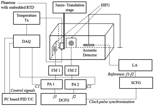
Figure 9. Variation of the acoustic amplitude with Δf at different temperatures for the PVA phantom.

Test using the agarose phantom

The agarose sample is prepared following the recipe given in reference [49]. An appropriately trimmed sample is loaded in a rheometer to measure the storage modulus while its temperature is varied in steps to cover the intended range. Figure 6 plots the measured storage modulus with temperature. A reason for choosing this phantom is that it mimicked human tissue well for its mechanical properties [49].

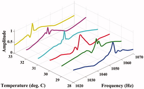
The experimental set-up for studying the shift of resonant mode(s) with temperature is shown in Figure 8. Fixing Δf, the variation of acoustic emission from the ROI with temperature is measured using a PVDF hydrophone (RP Acoustics PVDF RP 10I), the output of which is suitably amplified using a high-gain HVA-10 M-60-F A.C. amplifier to facilitate measurement. The frequency Δf itself is varied from 1020 Hz to 1070 Hz (for our present material), and the variation of the peak of the power spectrum with temperature is noted. The ambient temperature of the phantom was 26°C , and the temperature was varied from 28°C to 33°C. The results are plotted in Figure 10.

Figure 10. Variation of the acoustic amplitude with Δf at different temperatures for the agarose phantom.

It was seen during our experiments that the phantom made of agarose gets degraded (breaking of the gel, leading to changes that are irreversible) at higher temperatures beyond 36 °C. It is at 40 °C that we dissolve agarose powder en route to making the phantom. Hence, we have worked within 35 °C when experimenting with agarose phantoms. However, PVA phantoms remain quite stable even for temperatures up to 50 °C. Therefore, when working with PVA phantoms we have heated them up to 41 °C.

Results

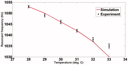
Figures 11 and 12 show the variation of the computed modal frequencies with temperature for different modes, in the cases of the PVA and agarose phantoms, respectively. Also shown is the experimentally obtained variation, which is seen to match well with the variation of one of the modes, the thirtieth for PVA and the eighteenth for agarose. The modes selected are shear modes. Strictly, we have not selected them, but found them through the match observed between experimental resonant frequency vs. temperature curve and its simulated counterparts for different modes (see Figures 11 and 12). We would also like to note that the corresponding shear waves are always tightly confined to the location of the US focal region, and the variations thereof should be through parameters of the region, including temperature. (It is also to be noted that the excited mode primarily corresponds to a shear mode of vibration of the ROI that in turn modulates the vibro-acoustic waves, reaching the boundary as explained in reference [29]. The other modes such as torsional modes and compressional modes, although excited due to ultrasonic forcing, do not play any significant role in modulating the vibro-acoustic wave, which is the carrier of information from the ROI to the surface in our measurement.) Therefore, Figures 13 and 14, which are our “transduction curves” for the two objects, give the readout for local temperature in terms of the resonant frequency. The standard deviations recorded in these figures show that the measurements are repeatable.

Figure 11. Variation of computed and captured modes with temperature for the PVA phantom.

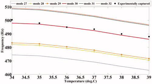
Figure 12. Same as Figure 11, but for the case of the agarose phantom.

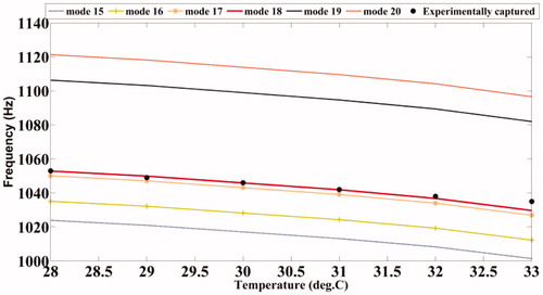
Figure 13. Experimentally observed variation of a resonant mode of ROI with temperature for the PVA phantom. This captured mode closely matches the thirtieth mode of the ROI obtained through simulation.

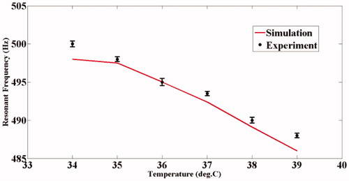
Figure 14. Same as Figure 13, but for the agarose phantom. This experimentally captured mode matches with the eighteenth mode of the ROI during the simulation.

Discussion

We have demonstrated the working of a remote temperature measurement system suitable for hyperthermia applications, the accuracy and repeatability of which are demonstrated through simulations and experiments on phantoms. One source of inaccuracy, however, is the hysteresis observed in rheometer measurements of temperature cycling (Figure 6). Notwithstanding the above, the performance of the present system is either comparable to or surpasses the existing temperature measurement systems. In the “Introduction”, we have cited a number of non-invasive temperature monitoring systems over which the presently developed one has certain advantages in the hyperthermia application, the main one being its ability to monitor temperature precisely at the region of heat application without the need for a separate “imaging” system. For comparison of performance, we quote some of the indices such as accuracy, repeatability and response time reported in the literature of existing systems (see also Introduction). Currently used systems for temperature monitoring employ either ultrasound thermometry or MR imaging. In ultrasound thermometry, one uses (1) the shift in input ultrasound pulse echo that depends on changes in the speed of sound and the thermal expansion coefficient of tissue with temperature; (2) the transmitted intensity change owing to the variation of the ultrasound attenuation coefficient with temperature and (3) back-scattered US energy changes with temperature. The MRI-based method utilises the change in proton resonance frequency (PRF) with temperature. Of these, MRI has the fastest response time, typically 438 ms in an application involving temperature mapping of a rat thigh while heating it with focussed ultrasound [50]. US thermometry, on the other hand, is not known for its fast response time, which is also true for the present system. For accuracy of measurement, MRI scores the best (accuracy of ±0.37⁰C has been reported in laboratory experiments with live animals [50]), followed by back-scattered energy monitoring (0.5 °C over a range of 25 °C to 43 °C that includes the hyperthermia range [51]). For the rest, the values are ±1% for a range of 5–65 °C (using changes in the speed of sound) and ±10% for the same range (using attenuation coefficient changes) [52]. The corresponding value for the present system is 0.3 °C over 34 °C to 39 °C for PVA and over 28 °C to 33 °C for agarose. However, there is no information available on the repeatability of measurements of existing systems. In the present case, with the precaution to avoid cycling of temperature because of the small residual hysteresis as mentioned, the measurements were found to be repeatable to a high accuracy (see also Figures 13 and 14).

We would like to mention in passing that we made attempts to demonstrate the working of the remote measurement on actual tissue samples through in vitro measurements on pork muscles and fat. We have, in fact, observed a shift in resonant frequencies with temperature as anticipated, but choose not to report this for lack of calibration. Our attempt to calibrate by inserting an RTD in tissue for independent tracking of temperature was a failure. This was due to the alteration of the resonant frequencies of the insonified focal region caused by the incision required for the insertion of a transducer. (For phantom studies, the insertion of RTD was done while moulding before solidification.) In addition to this, leakage of the ambient buffer solution into the region upsets calibration. The solution is to have a non-interfering alternative calibration such as MRI that can detect temperature changes. Unfortunately, we did not have access to an MRI system to complete this calibration, which is left for the future as part of an ongoing instrument development programme.

Considering the practical scenario wherein the tissue medium has heterogeneous acoustic properties, it is important to account for these first while arriving at the pressure distribution of the focal region, solving the Westervelt equation, and then modelling the transmittance of the measurement signal to the detector through the inhomogeneity. The inhomogeneity in the tissue will alter the quantitative accuracy as well as the spatial distribution of focal region pressure. Intensity changes will alter the strength (but not the location) of the resonant modes and thus do not affect the accuracy of the present measurements. Spatial distribution, however, alters the shape of the vibrating region affecting the modal frequencies, which will have a deleterious effect on the accuracy of the proposed measurement.

Secondly, the acoustic spectrum as detected in these experiments is essentially the spectrum of the vibrating region of interest (VROI) multiplied by the “transfer function” of the intermediate medium between the source and the tissue boundary, which is the background object (denoted as H(ω) in reference [27]). As a spectral shift is associated with modulation in the “time domain”, a shift in the locations of the modal frequencies is only expected when the background objects have periodic “grating-like” structures in them that can possibly modulate the emanating acoustic wave. Since such types of structures are unusual for an actual tissue, any effect on the present measurement from transmission through the background is trivial.

The heating-history dependent behaviour shown in Figure 6 is indicative of a non-trivial role played by the non-equilibrium aspects of the associated thermodynamics en route to a history-dependent modification of the spring-type internal forces offered by the material. For instance, in case a generalised Langevin dynamic model is adopted to describe the phenomena [53], a history-dependent multiplicative noise term may arise that would alter the local stiffness of the material. Furthermore, a fluctuation relation expressed in terms of the associated entropy production [54] may, in principle, be exploited to characterise this hysteresis. A detailed exploration of these issues is, however, beyond the scope of this work. Indeed, this hysteresis may carry over to our transduction curves as well. We caution that, though the deviation due to hysteresis is small, one should be aware of its effect, especially when a controller tries for the set point through cycling the temperature around it.

In the event of actual hyperthermia being performed on a patient, a phased array high intensity ultrasonic transducer can be employed for remote temperature measurement of different regions within the tumour at the same time. This measured temperature distribution can be used as a feedback to a control system to distribute the heat uniformly throughout the tumour volume. The method, being frequency based, does not suffer from signal corruption due to noise, as in the case with amplitude-based measurements.

Conclusions

The technique described in this paper may serve the dual purpose of heating the tumour and, more importantly, providing a patient friendly solution to the remote measurement of tumour temperature. We have been able to readout the temperature with the help of the natural frequency of vibration of the ultrasound focal volume, albeit with a small amount of hysteresis on temperature cycling, an analysis of which would, in itself, be an interesting future study. This technique can also be employed in any other hyperthermia systems employing other means of heating. In only such cases, the high intensity transducers may be replaced by low intensity ultrasonic sources. Variations in the elastic properties with temperature change during tests on two different phantom materials have been presented in this work. A somewhat classical modelling of the ROI has been done to compute the shift in its resonant frequency at various temperatures. The theoretically calculated shifts have had a high degree of agreement with their experimentally obtained counterparts. Implementation of this technique with a phased array HIFU transducer and an appropriate temperature control algorithm for multiple points will make cancer treatment with hyperthermia more patient friendly and effective.

Disclosure statement

No potential conflict of interest was reported by the authors.

References

- Hildebrandt B, Wust P, Ahlers O, et al. (2002). The cellular and molecular basis of hyperthermia. Crit Rev Oncol/hematol 43:33–56.
- van der Zee J. (2002). Heating the patient: a promising approach?. Ann Oncol 13:1173–84.
- Wust P, Hildebrandt B, Sreenivasa G, et al. (2002). Hyperthermia in combined treatment of cancer. Lancet oncol 3:487–97.
- Rhoads JE. (1983). Cancer – principles & practice of oncology. Ann Surg 197:116.
- Falk M, Issels R. (2001). Hyperthermia in oncology. Int J Hyperthermia 17:1–18.
- Gunderson LL, Tepper JE, Bogart JA. (2015). Clinical radiation oncology. Philadelphia: Elsevier Health Sciences.
- Kapp DS, Hahn GM, Carlson RW. (2000). Principles of hyperthermia.
- VanBaren P, Ebbini E. (1995). Multipoint temperature control during hyperthermia treatments: theory and simulation. IEEE Trans Biomed Eng 42:818–27.
- Seip R, Ebbini ES. (1995). Noninvasive estimation of tissue temperature response to heating fields using diagnostic ultrasound. IEEE Trans Biomed Eng 42:828–39.
- Hijnen NM, Heijman E, Köhler MO, et al. (2012). Tumour hyperthermia and ablation in rats using a clinical MR‐HIFU system equipped with a dedicated small animal set‐up. Int J Hyperthermia 28:141–55.
- Salomir R, Palussière J, Vimeux FC, et al. (2000). Local hyperthermia with MR‐guided focused ultrasound: Spiral trajectory of the focal point optimized for temperature uniformity in the target region. J Magn Reson imaging 12:571–83.
- Bing C, Nofiele J, Staruch R, et al. (2015). Localised hyperthermia in rodent models using an MRI-compatible high-intensity focused ultrasound system. Int J Hyperthermia 31:813–22.
- Peek M, Ahmed M, Scudder J, et al. (2016). High intensity focused ultrasound in the treatment of breast fibroadenomata: results of the HIFU-F trial. Int J Hyperthermia 32:881–8.
- Kaye EA, Monette S, Srimathveeravalli G, et al. (2016). MRI-guided focused ultrasound ablation of lumbar medial branch nerve: Feasibility and safety study in a swine model. Int J Hyperthermia 32:786–94.
- Thiburce AC, Frulio N, Hocquelet A, et al. (2015). Magnetic resonance-guided high-intensity focused ultrasound for uterine fibroids: Mid-term outcomes of 36 patients treated with the Sonalleve system. Int J Hyperthermia 31:764–70.
- Zhang L, Zhang W, Orsi F, et al. (2015). Ultrasound-guided high intensity focused ultrasound for the treatment of gynaecological diseases: a review of safety and efficacy. Int J Hyperthermia 31:280–4.
- Aptel F, Lafon C. (2015). Treatment of glaucoma with high intensity focused ultrasound. Int J Hyperthermia 31:292–301.
- Novell A, Al Sabbagh C, Escoffre J-M, et al. (2015). Focused ultrasound influence on calcein-loaded thermosensitive stealth liposomes. Int J Hyperthermia 31:349–58.
- Seip R, VanBaren P, Cain CA, Ebbini ES. (1996). Noninvasive real-time multipoint temperature control for ultrasound phased array treatments. IEEE Trans Ultrason Ferroelectr Freq Control 43:1063–73.
- Fossheim SL, Il'yasov KA, Hennig J, Bjørnerud A. (2000). Thermosensitive paramagnetic liposomes for temperature control during MR imaging-guided hyperthermia: in vitro feasibility studies. Acad radiol 7:1107–15.
- Quesson B, de Zwart JA, Moonen CT. (2000). Magnetic resonance temperature imaging for guidance of thermotherapy. J Magn Reson Imaging 12:525–33.
- El-Sharkawy A-MM, Sotiriadis PP, Bottomley PA, Atalar E. (2006). Absolute temperature monitoring using RF radiometry in the MRI scanner. IEEE Trans Circuits Syst I Regul Pap 53:2396–404.
- Conway J. (1987). Electrical impedance tomography for thermal monitoring of hyperthermia treatment: an assessment using in vitro and in vivo measurements. Clin Phys Physiol Meas 8:141.
- van Dongen KW, Verweij MD. (2011). A feasibility study for non-invasive thermometry using non-linear ultrasound. Int J Hyperthermia 27:612–24.
- Bing C, Staruch RM, Tillander M, et al. (2016). Drift correction for accurate PRF-shift MR thermometry during mild hyperthermia treatments with MR-HIFU. Int J Hyperthermia 32:673–87.
- Fatemi M, Greenleaf JF. (1998). Ultrasound-stimulated vibro-acoustic spectrography. Science 280:82–5.
- Fatemi M, Greenleaf JF. (1999). Vibro-acoustography: an imaging modality based on ultrasound-stimulated acoustic emission. Proc Nat Acad Sci 96:6603–8.
- Fatemi M, Greenleaf JF. (2000). Probing the dynamics of tissue at low frequencies with the radiation force of ultrasound. Phys Med biol 45:1449.
- Mazumder D, Umesh S, Vasu RM, et al. (2016). Quantitative vibro-acoustography of tissue-like objects by measurement of resonant modes. Phys Med Biol 62:107.
- Inaba S, Kumazaki H, Horibe M, Hane K. (1994). Temperature dependence of resonance frequency of shape-memory alloy vibrated photothermally. Jpn J Appl phys 33(9R):5064.
- Shiraishi N, Kimura M, Ando Y. (2014). Resonant frequency temperature dependence of polymer-based cantilever sensor for monitoring VOC. 9th International Workshop on microfactories, INMF 2014. p. 146–50. Available from: http://conf.papercept.net/images/temp/IWMF/media/files/0012.pdf
- Landsberger B, Hamilton M. (2001). Second-harmonic generation in sound beams reflected from, and transmitted through, immersed elastic solids. J Acous Soc Am 109:488–500.
- Aanonsen SI, Barkve T, Tjo JN. (1984). Distortion and harmonic generation in the nearfield of a finite amplitude sound beam. J Acous Soc Am 75:749–68.
- Tjo JN. (1987). Interaction of sound waves. Part I: Basic equations and plane waves. J Acous Soc Am 82:1425–8.
- Hamilton MF, Blackstock DT (eds.) (1998). Nonlinear acoustics. Boston: Academic press. 245.
- Rienstra SW, Hirschberg A. (2003). An introduction to acoustics. Eindhoven, Netherlands: Eindhoven University of Technology; 18:19.
- Westervelt PJ. (1963). Parametric acoustic array. J Acous Soc Am 35:535–7.
- Kamakura T, Ishiwata T, Matsuda K. (2000). Model equation for strongly focused finite-amplitude sound beams. J Acous Soc Am 107:3035–46.
- http://sonicconcepts.com/wp-content/uploads/2016/05/H-%C3%BF64_DataSheet_B.pdf
- Nightingale KR, Palmeri ML, Nightingale RW, Trahey GE. (2001). On the feasibility of remote palpation using acoustic radiation force. J Acous Soc Am 110:625–34.
- Konofagou E, Thierman J, Hynynen K. (2001). A focused ultrasound method for simultaneous diagnostic and therapeutic applications – a simulation study. Phys Med Biol 46:2967.
- Roy D, Rao GV. (2012). Elements of structural dynamics: a new perspective. Chichester, UK: John Wiley & Sons.
- Visscher WM, Migliori A, Bell TM, Reinert RA. (1991). On the normal modes of free vibration of inhomogeneous and anisotropic elastic objects. J Acous Soc Am 90:2154–62.
- Ďoubal S, Klemera P, Semecký V, et al. (2004). Non-linear mechanical behavior of visco-elastic biological structures–measurements and models. Biophysical DAYS 47:297–300.
- Wu CZ, Parker KJ. (2005). Shear wave interferometry, an application of sonoelastography. J Acous Soc Am 117:2587.
- Barnes HA, Hutton JF, Walters K. (1989). An introduction to rheology: Amsterdam, Netherlands: Elsevier.
- Kharine A, Manohar S, Seeton R, et al. (2003). Poly(vinyl alcohol) gels for use as tissue phantoms in photoacoustic mammography. Phys Med Biol 48:357.
- Hassan CM, Peppas NA. (2000). Structure and applications of poly (vinyl alcohol) hydrogels produced by conventional crosslinking or by freezing/thawing methods. In: Biopolymers· PVA Hydrogels, Anionic Polymerisation Nanocomposites. Berlin Heidelberg: Springer. 37–65.
- D’Souza WD, Madsen EL, Unal O, et al. (2001). Tissue mimicking materials for a multi-imaging modality prostate phantom. Medical physics 28:688–700.
- de Zwart JA, Vimeux FC, Delalande C, et al. (1999). Fast lipid-suppressed MR temperature mapping with echo-shifted gradient-echo imaging and spectral-spatial excitation. Magn Reson med 42:53–9.
- Simon C, VanBaren P, Ebbini ES. (1998). Two-dimensional temperature estimation using diagnostic ultrasound. IEEE Trans Ultrason Ferroelectr Freq Control 45:1088–99.
- Bamber J, Hill C. (1979). Ultrasonic attenuation and propagation speed in mammalian tissues as a function of temperature. Ultrasound Med biol 5:149–57.
- Sarkar S, Chowdhury SR, Roy D, Vasu RM. (2015). Internal noise-driven generalized Langevin equation from a nonlocal continuum model. Phys Rev E 92:022150.
- Crooks GE. (1999). Excursions in statistical dynamics. Doctoral dissertation. Berkeley, CA: University of California at Berkeley.