Optical flow and image segmentation analysis for noninvasive precise mapping of microwave thermal ablation in X-ray CT scans - ex vivo study

Abstract

Purpose: To develop image processing algorithms for noninvasive mapping of microwave thermal ablation using X-ray CT.

Methods: Ten specimens of bovine liver were subjected to microwave ablation (20–80 W, 8 min) while scanned by X-ray CT at 5 s intervals. Specimens were cut and manually traced by two observers. Two algorithms were developed and implemented to map the ablation zone. The first algorithm utilises images segmentation of Hounsfield units changes (ISHU). The second algorithm utilises radial optical flow (ROF). Algorithm sensitivity to spatiotemporal under-sampling was assessed by decreasing the acquisition rate and reducing the number of acquired projections used for image reconstruction in order to evaluate the feasibility of implementing radiation reduction techniques.

Results: The average radial discrepancy between the ISHU and ROF contours and the manual tracing were 1.04±0.74 and 1.16±0.79mm, respectively. When diluting the input data, the ISHU algorithm retained its accuracy, ranging from 1.04 to 1.79mm. By contrast, the ROF algorithm performance became inconsistent at low acquisition rates. Both algorithms were not sensitive to projections reduction, (ISHU: 1.24±0.83mm, ROF: 1.53±1.15mm, for reduction by eight fold). Ablations near large blood vessels affected the ROF algorithm performance (1.83±1.30mm; p < 0.01), whereas ISHU performance remained the same.

Conclusion: The two suggested noninvasive ablation mapping algorithms can provide highly accurate contouring of the ablation zone at low scan rates. The ISHU algorithm may be more suitable for clinical practice as it appears more robust when radiation dose reduction strategies are employed and when the ablation zone is near large blood vessels.

Keywords:

• Microwave
• thermal ablation
• X-ray CT
• thermal monitoring
• noninvasive

Introduction

According to an estimation of the American Cancer Society, 1.6 million new cases of cancer are diagnosed each year in the US alone, with a mortality of more than 35% [1]. In many cases the cancer is manifested as a tumour growth. Consequently, tumour removal or destruction is a major clinical challenge. Although surgery is the default option in most cases, it is not always desired or possible to operate [2]. Accordingly, there is a continuous effort to develop alternative minimal intervention methods for tumour treatment.

Thermal ablation therapy is an increasingly accepted minimal invasive option for the treatment of focal tumours in the liver, kidney and lung [3,4]. With this option, a needle type applicator is inserted into the body under image guidance. Thermal changes are then induced by either freezing the target [5,6] or heating it. Heating is commonly induced using radio frequency (RF) or microwave (MW) radiation. Continuous noninvasive monitoring with high temporal resolution is essential during the therapeutic procedure to verify whether the target tissue is adequately ablated and the damage to surrounding healthy tissue is minimised [7].

The most clinically mature technology available today for thermal monitoring is MRI [8–10]. However, MRI is an expensive imaging modality and imposes severe restrictions on the types of equipment that can be used for the procedure. Ultrasound is cost effective, hazardless and provides real time imaging. However, it has typically low signal to noise ratio (SNR) which leads to low accuracy in monitoring of the ablation boundaries [11,12]. Moreover, it has limited capability in imaging structures containing bones or gas. X-ray CT on the other hand is a widely available imaging modality, with high temporal and spatial resolution, is substantially less expensive than MRI and provides image quality which is superior to ultrasound. Additionally, it can also image the brain and lungs which ultrasound cannot and does not impose any restrictions on the equipment located in its vicinity. Furthermore, CT is particularly suitable for image guided robotic surgery [13,14]. Hence, when maintaining acceptable radiation levels, X-ray CT may be a beneficial modality for noninvasive monitoring of thermal procedures. Indeed, the potential of X-ray CT for thermal monitoring has been noted by previous investigators and several studies have examined the changes to image grey levels, i.e., Hounsfield units (HU), stemming from thermal changes [15–18]. These studies have most often attempted to relate the HU to temperature. However, as the outcome of the procedure is tissue ablation, direct mapping of the ablated zone, i.e., providing the contour of the tissue region which has undergone an irreversible change within the CT image, may be more clinically beneficial than temperature mapping. Although, previous studies [19–21] have reported that accurate ablation estimation (average radius discrepancy <2 mm) can be achieved, results to date have been largely incomplete as only partial information such as maximal diameter or average radius has been provided. Yet, under most clinical conditions accurate three dimensional measurement including detailed contours of the ablation area may be critical. This is particularly true for high risk locations [22] or problematically located tumours [23]. Hence, it is desired to develop a non-invasive method that will be capable of depicting to the operating crew the accurate contour of the ablated area in each CT image.

In this study, two new alternative algorithms for fine ablation contour analysis are introduced. The algorithms are applicable for noninvasive monitoring of the ablation area outline using a temporal set of X-ray CT scans acquired during the treatment. These two algorithms were chosen after conducting a preliminary evaluation with several alternative segmentation methods of textural analysis such as changes in the entropy or changes in the statistical parameters of the CT values and were found to be most promising candidates for further evaluation. The first algorithm is based on image segmentation of Hounsfield units changes (ISHU), the second algorithm is based on radial optical flow (ROF). These two approaches were chosen based on our previous works which have shown CT textural changes [19] and tissue expansion [20] during ablation. In an era of radiation dose awareness, the need for possible reduction of radiation was also assessed increasing interval of input data and reducing the number of acquired projections for image reconstruction as we hypothesised that less comprehensive data acquisition may be sufficient for real-time assessment of the ablation process.

Materials and method

Experimental setup and data acquisition

In order to evaluate the two algorithms, ten microwave ablation procedures were performed in ex-vivo bovine specimens obtained from several animals. Each specimen was approximately 10 × 10 × 10 cm in size. It was placed within a unique apparatus especially built for this research (Figure 1). The apparatus provides a fixed setup in order to ensure reproducibility and consistency of the experiments and to provide spatial match between the X-ray CT cross-section images and the gross pathology slices. After the specimen was placed in the apparatus, the MW antenna (HS Amica probe 14 G, HS Hospital Service S.P.A., Rome, Italy) tip was inserted through a hole in the apparatus wall into the tissue and positioned precisely at the centre of the apparatus. The ablation was performed for a constant heating duration of 8 min in each experiment. Each specimen was heated at one out of four power levels: 20, 40, 60 or 80 Watts, respectively to enable evaluation of the algorithms for different sized ablations. During the thermal ablation the liver was scanned with a CT scanner (Brilliance, Philips Healthcare, Cleveland, OH) every 5 s. The tube voltage and current were 120 kVp and 50 mAs, respectively, for all scans. FOV of 160 mm for an image size of 512 x 512 pixels was used yielding voxel size of: 0.3125 mm x 0.3125 mm x 1 mm. Each helical scan covered 40 slices of 1 mm thickness without overlap, covering a total of 40 mm along the antenna axis. Overall, 97 scans were acquired per experiment yielding 3880 images per ablation.

Figure 1. A photograph of the special apparatus used in this research. (a) The MW antenna is positioned at the centre of the apparatus. (b) The stainless steel blades, which were used for the gross pathology cuts were inserted through the apparatus slits which were positioned to match the known X-ray CT slices.

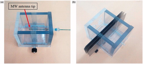
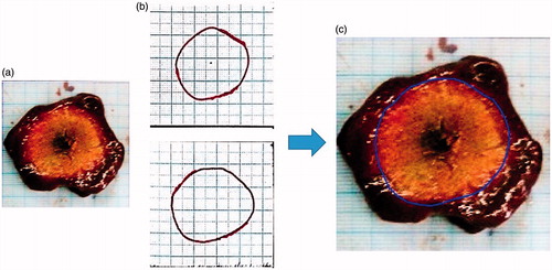
At the end of the ablation procedure, the specimen was sectioned with 10 mm spacing with thin steel blades inserted through the apparatus slits which were positioned to match the known X-ray CT slice coordinates (Figure 2). Each experiment provided 2–3 gross pathology sections through the ablation zone. Overall, 26 sections were obtained from all specimens. The contour of the ablated area was then manually traced on a transparent plastic sheet positioned atop the tissue and copied onto millimetric paper with a marked square region of 55 x 55 mm for calibration. The manual tracing was then digitally scanned and converted into black and white (BW) images for later comparison with the algorithm results. In addition, a scaled photograph of the gross pathology cross section was acquired. The photo was centred and calibrated to match the contour image and its number of pixels was decimated to match the number of pixels in the corresponding CT scan cross section (Figure 3). These contours served as the gold standard for comparison. Quantitative quality analysis was possible only to the cross sectional images which precisely matched the gross pathology cuts (2–3 images per case).

Figure 2. A pre-scan review image depicting the special apparatus with the MW antenna. Note the slits from both sides are used for inserting the stainless steel blades. The three dashed lines designate the planes used for comparison with the gross-pathology.

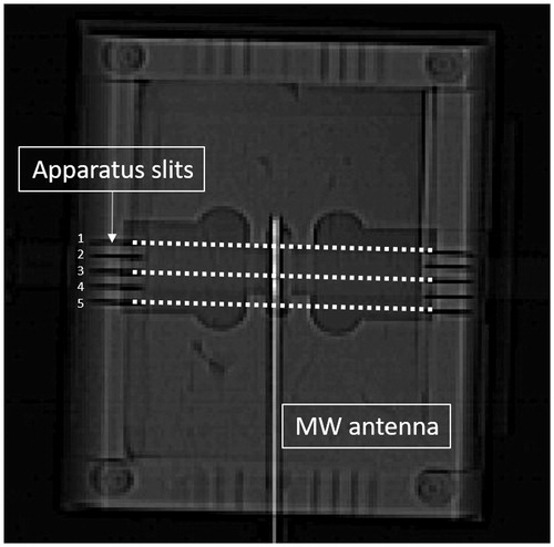
Figure 3. (a) A gross pathology cut. (b) The manual contours traced by two independent observers. (c) Graphic overlay of the average manual contour atop the calibrated gross pathology image. All images are 55 × 55 mm in size.

In order to examine inter-observer variability, sixteen slices were marked independently by two observers.

Algorithm I: image segmentation based on ISHU

All algorithms were implemented in MATLAB (MATLAB R2015a, Mathworks, Natick, MA).

In order to implement this algorithm, the following initial pre-processing stage was implemented: the antenna centre was automatically detected in each slice by making use of the fact that the metallic antenna demonstrates the highest HU values in the image. For every slice, the image was converted into a binary image. Using a connected components labeling (CCL) algorithm [24] an object corresponding to the antenna was detected and its centre of gravity was calculated and used for centring the image. Based on the detected antenna centres, the antenna axis in 3 D space was estimated using linear regression from a selected 55 x 55 mm sized region of interest (ROI) around this axis. In addition, a set of centred images corresponding to each single slice at all-time points was obtained. The algorithm was consequently examined on each temporal set (40 slices).

The algorithm consisted of the following steps:

1. Using the pre-treatment scan as a reference, a new set of centered images was generated by subtracting it from all images.

2. All the subtraction images, for each slice at all-time points, were summed up (Figure 4). This was done in order to enhance image feature changes and reduce the noise.

   Figure 4. Schematic depiction of the threshold selection procedure applied for the ISHU algorithm. (a) Subtracting the pre-treatment scan from all images. (b) Summing all subtracted images for each slice. (c) Select a ROI (red square) on the summed image which is outside the expected ablation zone. Set from this ROI a threshold value. (All images are 55 × 55 mm in size with the needle at the centre).

   

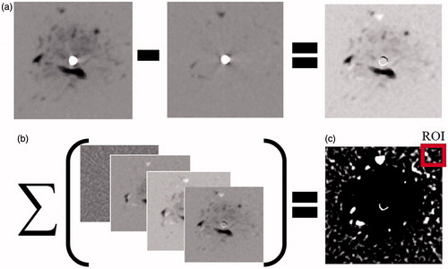
3. A 10 × 10 mm sized ROI located far from the antenna and outside the expected ablation zone was then selected in the summation image which was produced in the previous stage. It is assumed that any changes occurring outside the ablation zone are attributed to random scanning noise. Accordingly the reference zone needs to be sufficiently far from the ablated area in order to separate the random changes from changes caused by the ablation. The ROI was used for setting the threshold value. The threshold was determined by subtracting two standard deviations of the ROI grey levels from its mean value. This value statistically encompasses 97.72% of the background grey levels. Applying the threshold has yielded a binary image which emphasised the region around the antenna.

4. The binary image obtained in the stage 3 was then subjected to the following steps (see Figure 5):

   • “Holes” in the binary image were filled in using the “imfill” Matlab function, in order to obtain image continuity.

   • Using the CCL method a set of connected objects was generated.

   • The largest object located around the antenna centre was selected while all other were removed, in order to generate an image of a single object.

   • A median filter was then applied in order to smooth the object.

   Figure 5. The main stages of the ISHU algorithm. (a) Binary complement image based on the threshold. (b) The main blob after applying CCL and median filter. (c) Image b in a polar presentation using 10 degrees sectors to determine the radius of each sector. (d) The estimated ablation contour. (Images a, b and d are 55 × 55 mmin size).

   

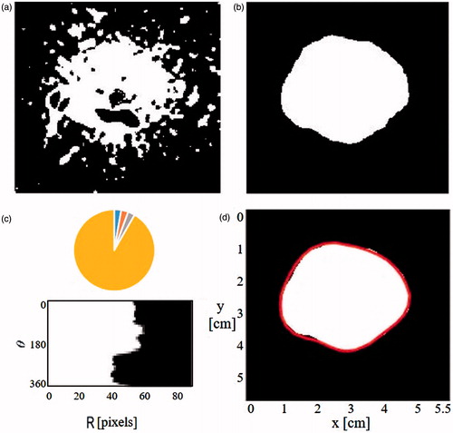
5. The output image from stage 4 was presented in a polar configuration using 10 degrees sectors. The average radius in each sector was calculated to yield a set of 36 radii around the antenna which were posited to represent the ablation zone boundaries (Figure 5). This was done in order to smooth the obtained contour demarcations and also to reduce the number of the required calculations.

6. The obtained contour was converted back into a Cartesian coordinate system and depicted as a graphical overlay atop the gross-pathology section picture along with the manual contour.

7. Finally, the obtained contours were compared to the gold standard as explained below.

Optical flow

Based upon the assumption that the ablation front expands radially relative to the antenna [20,21], the main idea of the optical flow algorithm is to detect radial textural changes occurring between two consecutive CT scans. For this purpose, we implemented the Lucas – Kanade optical flow method [25] on a polar presentation of the CT images.

In general, for a case of 2 D + t dimensions, a voxel located at (x, y, t) and with an intensity of I(x, y, t) will move at time t + Δ t between two consecutive frames by (Δx, Δy). Assuming that the brightness of the voxel is constant the following relation can be written: (1)

Also assuming that the movements are small, one can expand a Taylor series around the voxel to obtain: (2)

From Equations (1)(1) and (2)(2) it follows that: (3)

Dividing the equation by Δt yields: (4)

This can be rewritten as: (5)

Designating I_x, I_y, I_t as the partial derivatives of I(x, y, t) by ∂x,∂y,∂t respectively and V_x,V_y as the velocities along the x, y directions, respectively, this equation can be written as: (6)

Equation (6)(6) is defined as the optical flow equation. From this equation the optical flow velocities V_x, V_y can be calculated.

The Lucas–Kanade method for solving the optical flow equation assumes that the displacement of a voxel located at point p will constrain the voxels within its neighbourhood to move in a matching displacement. As a result, the optical flow equation holds for all voxels within a small window around point p. Therefore, the flow vector (V_x, V_y) is the solution to the following system of equations: (7)

Where, q1_,…,q_n are the location indices of the voxels within the window and I_x(q),I_y(q),I_t(q) are the corresponding partial derivatives at point q as explained above.

The matrix form of Equation (7)(7) is given by: (8)

The least squares solution for Equation (8)(8) is given by [25]: (9)

When converting the images into a polar coordinate system (r,φ), the flow components become the radial V_r and tangential V_φ velocities, i.e., .

In this study we focussed primarily on the radial velocity V_r as noted above.

Algorithm II: ROF

The first stage of the optical flow algorithm was identical to the pre-processing stage described above for the image segmentation algorithm. Thereafter, the algorithm processing continued as follows (see Figure 6):

Figure 6. The main stages of the ROF algorithm. (a) Convert all images into polar presentation using 10 degrees sectors. (b) Apply the Lukas- Kanade optical flow method on every two consecutive scans to obtain a radial flow map where red represents an area with high flow value. (c) Sum all the flow maps acquired for each slice at all time points and choose reference radius (red line). (d) Thresholded image. (e) The red line represents the ablation front.

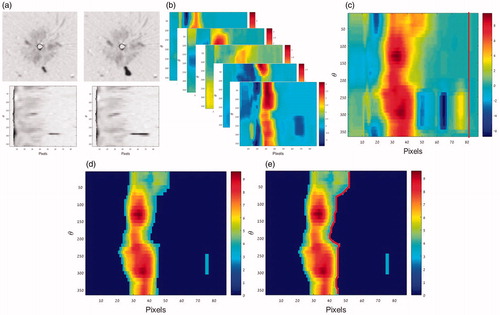
1. All subtraction images were converted into a polar presentation using 10 degrees sectors.

2. The Lukas-Kanade optical flow method was applied on every two temporally consecutive scans of the same slice, using a window of 11 × 11 pixels (about 3 × 3 mm). It is postulated that the pixels which depict the most significant changes are those located at and near the border zone. Hence, the ROF actually tracks the border propagation. By considering only the radial flow V_r in the polar images, a radial flow map was obtained.

3. All the obtained flow maps for each slice at all-time points were summed, i.e., all the frames obtained for that slice.

4. A reference radius which is much larger than the expected ablation zone was then chosen. According to the data reported by Hines-Peralta et al. [26] the short axis radius for 8 min duration and power of 100 watt is 23 ± 0.5 mm. Hence, it should be smaller for lower power levels. In our case the duration was similar (8 min), but the maximal power applied was 80 watt. Nonetheless, to be on the safe side, the reference radius was set here to 26 mm. The average and standard deviation of the optical flow values for that reference radius were calculated. These flow values are expected to stem from noise only. The threshold was subsequently determined by adding two standard deviations to the mean value of that optical flow value. All values below the threshold were nulled.

5. For each angular sector, the largest radius which depicted optical flow value above the threshold was considered to represent the ablation front.

6. The ablation contour was then presented as a vector and was filtered using discrete cosine transform (DCT). The cut-off point was set at 50% of the DCT coefficients.

7. Finally, the obtained contour was converted back into a Cartesian coordinate system and depicted as a graphical overlay atop the gross-pathology section picture along with the manually traced contour. The results were quantitatively compared to the gold-standard as noted below.

Quality analysis

Finally, the two manually traced contours were also converted into a polar presentation and averaged for the corresponding 36 angular sectors. This was done in order to obtain a comparable accuracy with the automatic contours. The mean contour was used as a gold-standard for quantitative comparison to the automatic boundary detection. Comparison was possible only to the cross sectional images which precisely matched the gross pathology cuts (2–3 images per case).

Three numerical indices were used: (i) Average absolute radial discrepancy, |ΔR|, between the gold-standard Rm_i and the automatically obtained contour R_ai using the Equation (10)(10) , for 36 angular sectors of 10 degrees in each of the 16 slices (576 sectors altogether): (10)

(ii) The maximal over-estimation, i.e., the largest positive radial discrepancy of the automatic contour which exceeded the gold-standard. (iii) The maximal under-estimation, i.e., the largest negative radial discrepancy where the gold-standard exceeded the automatic contour.

Sensitivity analysis of the algorithms to the spatiotemporal sampling rate

The motivation for the sensitivity analysis stems was from the need to minimise the ionising radiation absorbed during the treatment. Accordingly, it is desired to know by how much the number of acquisitions can be reduced while still retaining the essential information needed to perform the ablation contour analysis with an acceptable accuracy.

Changes in two parameters were evaluated: (i) scan acquisition rate, i.e., the time interval between two consecutive scans and (ii) the number of projections obtained in a single acquisition. Both methods were evaluated offline from the entire scan data, where partial data was used, instead of the full acquisition data.

Initially, out of the 97 scans acquired during the 8 min of ablation in each case, subsets of scans representing time intervals of 1, 2, 4 and 8 min (which is equivalent to relative dose (RD) of 0.5, 0.25 and 0.125 respectively) were selected. The analysis was consequently performed on these subsets and the accuracy of the analysis was evaluated as a function of scan acquisition rate.

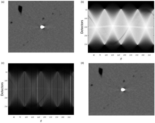
The second analysis was performed by generating a sinogram (Radon transform) for each acquired frame. The sinogram was then down sampled by factors of 2, 4 and 8, by choosing subsets from the Radon sinogram. Using the inverse Radon transform new sets of images (with lower quality) were generated and analysed (Figure 7). The corresponding obtained contours were compared to the gold standard so the performances of both algorithms can be compared with each other.

Figure 7. Exemplary image obtained by artificially reducing the number of projections. (a) Originally acquired X-ray CT image. (b) Radon transform of image a. (c) Down sampled Radon transform by a factor of four. (d) Inverse Radon transform of image c.

Results

Inter-observer variability of gross pathology contouring

The sizes of the ablation diameters measured were 2.75 ± 0.29 mm for ablation at 20 Watts, 3.34 ± 0.29 mm for 40 Watts, 3.68 ± 0.44 mm for 60 watts and 4.27 ± 0.34 mm for 80 Watts. The obtained average absolute value of the radial discrepancy and its standard deviation were 1.35 ± 0.91 mm, respectively. There was no significant difference between the observers (t-test, p > 0.05).

Algorithm I: ISHU

The image segmentation algorithm was implemented to the entire data set (which comprised of 38 800 images =10 cases x 97 scans x 40 slices). The algorithm ran smoothly without any notable complications. Run time was 0.159 s per slice. Representative results are depicted in Figure 8. The overall results are summarised in Table 1 for all power levels. The mean absolute discrepancy obtained was: 1.04 ± 0.74 mm. The maximal over estimation and the maximal under estimation for the 26 trials averaged 2.51 ± 1.01 and −2.03 ± 0.78 mm and ranged from 0.76 to 3.75 mm and −3.34 to 0 mm respectively.

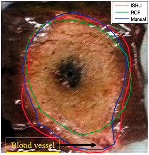
Figure 8. Exemplary results obtained by both algorithms and the corresponding average manual contours depicted atop the gross pathology images. All images are 55 × 55 mm in size.

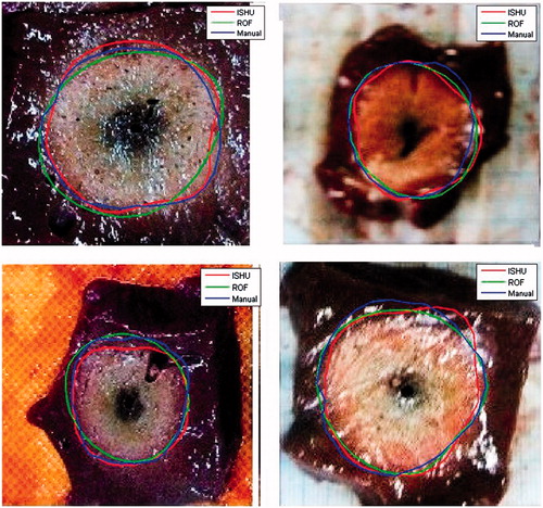
Table 1. Average results of the radial discrepancy for both algorithms depending on the power level for acquisition interval of 5 s.

Power	Ablation diameter (mm)	$\mathrm{I}\mathrm{S}\mathrm{H}\mathrm{U}:\left|\mathrm{\Delta }\mathrm{R}\right|\mathrm{m}\mathrm{m}$	$\mathrm{R}\mathrm{O}\mathrm{F}:\left|\mathrm{\Delta }\mathrm{R}\right|\mathrm{m}\mathrm{m}$
20 Watt	2.75±0.20	0.78±0.50	0.85±0.50
40 Watt	3.34±0.29	1.09±0.72	1.14±0.96
60 Watt	3.68±0.44	1.13±0.87	1.26±0.96
80 Watt	4.27±0.34	1.11±0.81	1.32±0.85
Total		1.04±0.74	1.16±0.79

Algorithm II: ROF

The ROF algorithm was implemented to the entire data set as well. Run time was 0.498 s per slice. Representative results are depicted in Figure 8. The average absolute discrepancy was: 1.16 ± 0.79 mm. The maximal over estimation and the maximal under estimation were comparable to the ISHU algorithm and ranged from 0 to 3.49 mm and −5.01 to 0 mm with an average of 2.06 ± 1.32 and −2.14 ± 1.53 mm, respectively. The overall results obtained for the different power levels are summarised in Table 1.

For this algorithm however, the performance was inadequate under certain conditions, specifically when the ablation site was proximal to a large blood vessel. For these cases, the average absolute discrepancy was: 1.83 ± 1.30 mm, compared to 1.00 ± 0.67 mm when no large blood vessels were in the ablation front vicinity.

Radiation dose reduction

The results of both algorithms depending on the acquisition interval are outlined in Table 2. As can be seen, the accuracy of the ISHU algorithm has not changed up to an interval of 2 min. For all intervals, the absolute mean discrepancy ranged from 1.04 ± 0.74 to 1.79 ± 1.10 mm. In this data arrangement, the ROF algorithm did not always perform smoothly. Specifically, when the time interval between the scans was set to 4 min, the algorithm yielded results in only 42% of the cases, likely stemming from the fact that the amount of data available was insufficient to calculate the temporal derivatives adequately. The ROF algorithm is not applicable for 8 min acquisition interval. The algorithm performed well for all other data sets and the absolute mean discrepancy ranged from 1.16 ± 0.79 to 1.76 ± 1.28 mm (values similar to the initial data set).

Table 2. Average results of the radial discrepancy for both algorithms depending on the acquisition interval.

Acquisition interval	Scans	$\mathrm{I}\mathrm{S}\mathrm{H}\mathrm{U}:\left|\mathrm{\Delta }\mathrm{R}\right|\mathrm{m}\mathrm{m}$	$\mathrm{R}\mathrm{O}\mathrm{F}:\left|\mathrm{\Delta }\mathrm{R}\right|\mathrm{m}\mathrm{m}$
5 s	97	$1.04\pm 0.74$	$1.16\pm 0.79$
1 min	9	$1.09\pm 0.76$	$1.49\pm 1.09$
2 min	5	$1.12\pm 0.85$	$1.76\pm 1.28$
4 min	3	$1.37\pm 0.96$	1.85±1.30*
8 min	2	$1.79\pm 1.10$	N/A

* The algorithm yielded results in only 11 cases out of 26.

The results examining the effect of reduction in the number of projections used for the image reconstruction are summarised in Table 3 for both algorithms. As can be noted, both algorithms were as accurate with the full Radon transform data set and the mean discrepancy ranged from 1.09 ± 0.76 to 1.24 ± 0.83 mm for the ISHU algorithm and 1.49 ± 1.09 to 1.53 ± 1.15 mm for the ROF algorithm. The acquisition interval for all data sets in this section was 1 min.

Table 3. Average results of the radial discrepancy for both algorithms depending on the number of projections (NP) used for the image reconstruction. The acquisition interval was 1 min.

NP	RD	$\mathrm{I}\mathrm{S}\mathrm{H}\mathrm{U}:\left|\mathrm{\Delta }\mathrm{R}\right|\mathrm{m}\mathrm{m}$	$\mathrm{R}\mathrm{O}\mathrm{F}:\left|\mathrm{\Delta }\mathrm{R}\right|\mathrm{m}\mathrm{m}$
1080	100%	$1.09\pm 0.76$	$1.49\pm 1.09$
540	$50\mathrm{\%}$	$1.13\pm 0.82$	$1.50\pm 1.11$
270	$25\mathrm{\%}$	$1.05\pm 0.74$	$1.51\pm 1.07$
135	$12.5\mathrm{\%}$	$1.24\pm 0.83$	$1.53\pm 1.15$

RD: the ratio between the number of projections in the current set and the original number of projections.

Discussion

In this study, two alternative algorithms for noninvasive thermal ablation monitoring by detailed contouring have been introduced. Both algorithms have yielded high accuracy for all power levels in ex-vivo experiments. Although techniques for ablation area mapping have been suggested for MRI and US [27–30], to the best of our knowledge, this is the first study which attempts to provide automated noninvasive ablation detailed contouring with precise bordering of the ablated zone using X-ray CT. This improves over previous studies results [19–21] which provided only partial information such as maximal diameter or average radius. Such analysis is highly important and may be crucial for evaluating the effectiveness of the treatment. Moreover, it can reduce the need for post-treatment injection of enhancing contrast agent and its corresponding imaging protocols. The fact that the established average accuracy is smaller than 2 mm in all of the studied cases and in the range of the inter-observer variability (in some cases even better) obtained by the manual tracing strongly indicates that such an approach may be potentially useful in the clinical setting. According to[31,32] there is no standardisation about the optimal margin size beyond the tumour border but currently 5–10 mm margin is recommended. In our case, if the ablation is stopped at 7.5 mm margin beyond the tumour border, an accuracy of 2 mm will ensure that ablated zone is within the recommended range.

The two suggested methods differ substantially in their computational approaches. While the ISHU algorithm is based on analysis of stationary changes in the Hounsfield units, the ROF algorithm investigates the dynamic motion of the ablation front as manifested in the derivatives of the image texture (This is particularly true for high risk locations [22] or problematically located tumours [23]. Hence, it is desired to develop a non-invasive method that will be capable of depicting the accurate contour of the ablated area in each CT image). Therefore, merger of the two contour types may not necessarily lead to a more accurate tracing, as can be clearly noted in Figure 8. Although both algorithms can potentially perform comparably well, each one has its own advantages and drawbacks. Whereas the ISHU is more robust and requires less computations, hence provides shorter run timesand relies upon a pre-selected reference zone. This zone needs to be chosen by the operator from the reference scan prior to the ablation procedure. Furthermore, this reference zone needs to be sampled from the same tissue/organ which is being treated. In addition, it has to be relatively homogenous and sufficiently far from the ablated area. This may pose a problem when treating small tumours located in isolated regions. The ROF on the other hand is fully automated and does not require any operator intervention. However, since it relays on temporal derivatives, it must have at least three scans acquired at different time points, (to obtain two subtraction images).

One of the obstacles encountered when implementing the ROF algorithm is its inadequate outcome when the ablation was located near a major blood vessel. Because of the ex-vivo setup, the blood vessels contained air. Consequently, a “chimney effect” [33,34] was generated whereby heat convection in the blood vessels was much faster than the heat conduction in the tissue. This causes the ablation front to have irregular features. As a result, the ROF algorithm which assumes radial expansion of the ablation front tends to ignore these regions of the ablation and the algorithm performance has been impaired (see Figure 9). This phenomenon is expected to occur less in in-vivo procedures, where “heat-sink” effect is more probable to occur [7,35,36].

Figure 9. Example of the “chimney effect” phenomenon. As can be noted the ROF algorithm ignores the regions of ablation that were caused by this phenomenon while the ISHU algorithm captures them.

One of the most important features that hinders an extensive use of X-ray CT as a monitoring modality is the naturally associated risk of ionising radiation. Nonetheless, based on current research in this field, it is anticipated that radiation dose will be substantially reduced for commercially available CT scanners in the near future [37], making X-ray CT monitoring and the suggested algorithm more attractive for routine clinical use. Today, there are several strategies for reducing radiation dose which can be divided into software based and hardware based strategies. The main software based strategy is applying iterative image reconstruction [38,39]. Some hardware strategies are based on changing the X-ray tube current in real-time, such as the tube current modulation (TCM) method or the automatic exposure control (AEC) [40,41]. Another approach is to use external collimators around the scanned object and reduce the number of acquired projections [42]. Our study focussed on two approaches for this purpose: (i) reduce the total number of scans acquired and (ii) reduce the number of projections acquired in each scan. In this study, we have examined the effect of implementing both approaches on the suggested algorithms.

Based upon our results, the ISHU algorithm appears to be more robust, it presents accurate outcome for all diluted data sets under both dose reduction strategies. This could imply that ISHU is more appropriate for use in protocols which involve dose reduction. Furthermore, since it can be applied under the constraints of both dose reduction strategies mentioned earlier, it is noted that an optimal protocol may potentially be found by combining the two dose reduction approaches.

The ROF algorithm on the other hand, is more sensitive to the reduction in the amount of data. This stems from the fact that a basic assumption in optical flow is that the changes between two successive images are small enough to implement the expansion by the Tylor series (Equation (3)(3) ). Hence, when the sampling interval is large this approximation may become less valid. As was observed in this study, it can be ineffective when the total number of acquisitions during the ablation is smaller than three scans. Nonetheless, it is expected that during clinical applications the number of acquisitions will be larger than three in order to provide real time feedback to the operator. Hence, the recommended approach for radiation dose reduction when using the ROF algorithm should be the projections reduction approach. This stems from the findings that the algorithm implementation on all diluted data sets yielded precise results comparable to the results obtained from the full Radon set.

In order to bring these imaging approaches to the next level and develop a clinical tool based on the ISHU or ROF algorithms, one must consider several issues: First, we will need to accelerate the algorithms run time so that it will be suitable for a real-time application. To attain this goal, one may use parallel coding, code translation into low-level programming language or use more powerful hardware such as GPU. Secondly, the algorithms should be examined under in-vivo conditions and extended to yield 3 D reconstruction. In such case, other quality metrics could potentially be more beneficial. For example: the Hausdorff distance or DICE indices. Thirdly, since the detectors of X-ray CT scanner are calibrated to work in a limited HU range of the human body composition, the metallic antenna, which has high attenuation, can cause severe artefacts that will influence the adjacent pixels and they will appear darker than their actual HU. This problem may be significant in cases of ablation of small objects where high accuracy in the vicinity of the antenna is necessary. Metal artefacts reduction methods are available today [43–47] and can be used for such cases. However, it should be taken into account that every use of additional algorithms will increase the computation time. Finally, the suggested algorithms were tested on X-ray CT scans acquired during a thermal ablation that was performed using MW antenna. Yet, there is no notable reason that the algorithms outcome will be affected when they are applied to a data sets acquired during other needle-type applicators such as RF or laser.

In conclusion, this study presents two alternative algorithms for noninvasive monitoring of thermal ablation procedures. Both algorithms provide highly accurate (average error <2 mm) detailed contours of the ablated area. When introduced to dose reduction strategies, the results of both algorithms were not affected substantially but the ISHU algorithm was more robust and stable, hence seems to be more suitable for such applications. Using this algorithm can potentially provide a real time accurate monitoring with reasonable radiation dose and can advance the use of thermal ablation as an alternative solution for surgery in tumour removal procedures.

Acknowledgments

This research was financially supported by the Israel Science Foundation [Grant No. 758/14]. In addition, the authors wish to acknowledge the financial support provided by the Technion-ITT. The authors would also like to thank Shem-Tov Halevi and Nathalie Greenbaum for their technical support.

Additional information

Funding

This research was financially supported by the Israel Science Foundation [Grant No. 758/14]. In addition, the authors wish to acknowledge the financial support provided by the Technion-ITT.

References

- Siegel RL, Miller KD, Jemal A. (2016). Cancer statistics, 2016. CA Cancer J Clin 66:7–30.
- Van Tilborg AAJM, Meijerink MR, Sietses C, et al. (2011). Long-term results of radiofrequency ablation for unresectable colorectal liver metastases: a potentially curative intervention. Br J Radiol 84:556–65.
- Dodd GD, Soulen MC, Kane RA, et al. (2000). Minimally invasive treatment of malignant hepatic tumors: at the threshold of a major breakthrough. Radiographics 20:9–27.
- Singletary S. (2001). Minimally invasive techniques in breast cancer treatment. Semin Surg Oncol 20:246–50.
- Gill IS, Remer EM, Hasan WA, et al. (2005). Renal cryoablation: outcome at 3 years. J Urol 173:1903–7.
- Hines-Peralta A, Hollander CY, Solazzo S, et al. (2004). Hybrid radiofrequency and cryoablation device: preliminary results in an animal model. J Vasc Interv Radiol 15:1111–20.
- Goldberg SN, Gazelle GS, Mueller PR. (2000). Thermal ablation therapy for focal malignancy: a unified approach to underlying principles, techniques, and diagnostic imaging guidance. AJR Am J Roentgenol 174:323–31.
- Hynynen K, McDannold N. (2004). MRI guided and monitored focused ultrasound thermal ablation methods: a review of progress. Int J Hyperthermia 20:725–37.
- Germain D, Chevallier P, Laurent A, Saint-Jalmes U. (2001). MR monitoring of tumour thermal therapy. Magn Reson Mater Phys Biol Med 13:47–59.
- Clasen S, Pereira PL. (2008). Magnetic resonance guidance for radiofrequency ablation of liver tumors. J Magn Reson Imaging 27:421–33.
- Gaitini D, Zivari M, Abadi S, et al. (2008). Evaluating Tissue changes with ultrasound during radiofrequency ablation. Ultrasound MedBiol 34:586–97.
- Correa-Gallego C, Karkar AM, Monette S, et al. (2014). Intraoperative ultrasound and tissue elastography measurements do not predict the size of hepatic microwave ablations. Acad Radiol 21:72–8.
- Abdullah BJJ, Yeong CH, Goh KL, et al. (2014). Robotic-assisted thermal ablation of liver tumours. Eur Radiol 25:246–57.
- Herrell SD, Kwartowitz DM, Milhoua PM, Galloway RL. (2009). Toward image guided robotic surgery: system validation. J Urol 181:783–90.
- Fani F, Schena E, Saccomandi P, Silvestri S. (2014). CT-based thermometry: an overview. Int J Hyperthermia 30:219–27.
- Li M, Abi-Jaoudeh N, Kapoor A, et al. Towards cone-beam CT thermometry. In: Holmes DR III, Yaniv ZR, editors. SPIE, Medical Imaging 2013: Image-Guided Procedures, Robotic Interventions, and Modeling. Bellingham, WA: SPIE; 2013. p. 86711I.
- Pandeya GD, Klaessens JHGM, Greuter MJW, et al. (2011). Feasibility of computed tomography based thermometry during interstitial laser heating in bovine liver. Eur Radiol 21:1733–8.
- Schena E, Saccomandi P, Giurazza F, et al. (2013). Experimental assessment of CT-based thermometry during laser ablation of porcine pancreas. Phys Med Biol 58:5705–16.
- Weiss N, Goldberg SN, Nissenbaum Y, et al. (2016). Noninvasive microwave ablation zone radii estimation using X-ray CT image analysis. Med Phys 43:4476–82.
- Weiss N, Goldberg SN, Nissenbaum Y, et al. (2015). Planar strain analysis of liver undergoing microwave thermal ablation using X-ray CT. Med Phys 42:372.
- Liu D, Brace CL. (2014). CT imaging during microwave ablation: analysis of spatial and temporal tissue contraction. Med Phys 41:113303.
- Teratani T, Yoshida H, Shiina S, et al. (2006). Radiofrequency ablation for hepatocellular carcinoma in so-called high-risk locations. Hepatology 43:1101–8.
- Chen MH, Yang W, Yan K, et al. (2008). Radiofrequency ablation of problematically located hepatocellular carcinoma: tailored approach. Abdom Imaging 33:428–36.
- Ronse C, Devijver PA. (1984). Connected components in binary images: the detection problem. Letchworth, Hertfordshire, England: Research Studies Press; New York: Wiley.
- Lucas BD, Kanade T. (1981). An iterative image registration technique with an application to stereo vision. Imaging 130:674–9.
- Hines-Peralta AU, Pirani N, Clegg P, et al. (2006). Microwave ablation: results with a 2.45-GHz applicator in ex vivo bovine and in vivo porcine liver. Radiology 239:94–102.
- Weidensteiner C, Quesson B, Caire-Gana B, et al. (2003). Real-time MR temperature mapping of rabbit liver in vivo during thermal ablation. Magn Reson Med 50:322–30.
- Samset E. (2006). Temperature mapping of thermal ablation using MRI. Minim Invasive Ther Allied Technol 15:36–41.
- Chen BT, Shieh J, Huang CW, et al. (2014). Ultrasound thermal mapping based on a hybrid method combining physical and statistical models. Ultrasound Med Biol 40:115–29.
- Fosnight TR, Hooi FM, Keil RD, et al. (2016). Echo decorrelation imaging of rabbit liver and VX2 tumor during in vivo ultrasound ablation. Ultrasound Med Biol 43:1–11.
- Brace C. (2011). Thermal tumor ablation in clinical use. IEEE Pulse 2:28–38.
- Munireddy S, Katz S, Somasundar P, Espat NJ. (2012). Thermal tumor ablation therapy for colorectal cancer hepatic metastasis. J Gastrointest Oncol 3:69–77.
- Lopresto V, Pinto R, Lovisolo GA, Cavagnaro M. (2012). Changes in the dielectric properties of ex vivo bovine liver during microwave thermal ablation at 2.45 GHz. Phys Med Biol 57:2309–27.
- Cavagnaro M, Pinto R, Lopresto V, et al. (2015). Numerical models to evaluate the temperature increase induced by ex vivo microwave thermal ablation. Phys Med Biol 60:3287–311.
- Yu NC, Raman SS, Kim YJ, et al. (2008). Microwave liver ablation: influence of hepatic vein size on heat-sink effect in a porcine model. J Vasc Interv Radiol 19:1087–92.
- Lu DSK, Raman SS, Vodopich DJ, et al. (2002). Effect of vessel size on creation of hepatic radiofrequency lesions in pigs: assessment of the “heat sink” effect. AJR Am J Roentgenol 178:47–51.
- Sarti M, Brehmer WP, Gay SB. (2012). Low-dose techniques in CT-guided interventions. Radiographics 32:1109–19.
- Leipsic J, Nguyen G, Brown J, et al. (2010). A prospective evaluation of dose reduction and image quality in chest CT using adaptive statistical iterative reconstruction. AJR Am J Roentgenol 195:1095–9.
- Silva AC, Lawder HJ, Hara A, et al. (2010). Innovations in CT Dose reduction strategy: application of the adaptive statistical iterative reconstruction algorithm. AJR Am J Roentgenol 194:191–9.
- Yu L, Liu X, Leng S, et al. (2009). Radiation dose reduction in computed tomography: techniques and future perspective. Imaging 1:65–84.
- Mc Collough C, Primak NA, Braun N, et al. (2009). Strategies for reducing radiation dose in CT. Radiol. Clin. North Am 47:27–40.
- Christner JA, Zavaletta VA, Eusemann CD, et al. (2010). Dose reduction in helical CT: dynamically adjustable z-axis X-ray beam collimation. Am J Roentgenol 194:49–55.
- Subhas N, Polster JM, Obuchowski NA, et al. (2016). Imaging of arthroplasties: improved image quality and lesion detection with iterative metal artifact reduction, a new CT metal artifact reduction technique. AJR Am J Roentgenol 207:378–85.
- Zhao S, Robeltson DD, Wang G, et al. (2000). X-ray CT metal artifact reduction using wavelets: an application for imaging total hip prostheses. IEEE Trans Med Imaging 19:1238–47.
- Wang G, Snyder DL, O’Sullivan JA, Vannier MW. (1996). Iterative deblurring for CT metal artifact reduction. IEEE Trans Med Imaging 15:657–64.
- Wu M, Keil A, Constantin D, et al. (2014). Metal artifact correction for X-ray computed tomography using kV and selective MV imaging. Med Phys 41:121910.
- Kennedy JA, Israel O, Frenkel A, et al. (2007). The reduction of artifacts due to metal hip implants in CT-attenuation corrected PET images from hybrid PET/CT scanners. Med Biol Eng Comput 45:553–62.