Two questions about the analysis and interpretation of randomised trials

Abstract

This non-technical tutorial focus on two questions about the analysis of data from randomised trials. Which is the more appropriate analysis of data from a randomised trial – an unadjusted analysis or an adjusted one? When a result is not statistically significant is it nevertheless appropriate to comment on its direction?

Keywords:

• Randomised trial
• statistical adjustment
• statistical significance

Introduction

The analysis and interpretation of data from randomised trials can be a source of confusion. Indeed, two questions can be particularly perplexing:

1. Which is the more appropriate analysis of data from a randomised trial – an unadjusted analysis or an adjusted one? More specifically: should the primary analysis always be the unadjusted one?

2. When a result is not statistically significant is it nevertheless appropriate to comment on its direction?

We discuss these questions, with a focus on pictures and general principles rather than technical details.

Question 1: statistical adjustment

Figure 1(a,b) illustrate two possible rationales for adjustment. The primary predictor variable is study group, illustrated by the different symbols. The outcome (response) variable is plotted on the y-axis. As drawn the outcome variable, labelled Y, is continuously scaled. The control variable (i.e., the covariate) is plotted on the x-axis. As drawn there is a single continuously scaled covariate, labelled Z, although nothing fundamental changes if there are more or differently scaled variables except that the figures becomes more complex.

Figure 1. (a) Illustration of an unbalanced covariate. (b) Illustration of a balanced covariate.

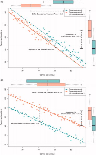
The main difference between Figure 1(a,b) is the degree to which the two study groups are balanced on the covariate: Figure 1(a) is unbalanced whereas Figure 1(b) is balanced. Because randomisation tends to produce (approximate) balance between the study groups Figure 1(b) is more typical of randomised trials, although Figure 1(a) is possible for trials with small sample sizes, or small subgroups within larger trails, or large trials with extraordinarily bad luck. Figure 1(a) can also occur when randomisation is unsuccessful – for example, when study personal have discovered the randomisation scheme and, whether intentionally or not, preferentially enrol subjects depending upon which treatment they will receive. Within the context of randomised trials, preventive measures include hiding the randomisation scheme, making decisions about inclusion and exclusion before randomisation and stratified or blocked sampling (i.e., often intended to ensure approximate balance, even within small subgroups). Figure 1(a) often describes non-randomised observational studies, which tend to have less balance than randomised trials.

The imbalance in Figure 1(a) is illustrated by the differences in the boxplots at the top of the figure, whereas the balance in Figure 1(b) is illustrated by their similarity.

As drawn, in Figure 1(a) the unadjusted comparison is based on the boxplots to the right of the figure. These were drawn by ignoring the covariate, and simply plotting the value of the outcome variable (i.e., in a single dimension). More specifically, the unadjusted comparison is the difference between the mean values of Y in the two groups, as illustrated in the figure. The unadjusted comparison suggests that outcomes are larger in group B.

In contrast, the adjusted comparison takes into account the imbalance between the covariates (technically, by applying an analysis of covariance for which the predictors are study group, usually denoted by X, and the covariate Z). Graphically, this is equivalent to first fitting regression lines that summarise the relationship between Z and Y, and then calculating the vertical distance between these lines (which, for simplicity of presentation, are assumed to have the same slopes, and thus, the question of “interaction” need not be considered). The “adjusted” comparison suggests that outcomes are larger in group A. More generally, the figure illustrates that the analysis of covariance adjusts for the imbalance between the groups by making the comparison at identical values of Z (and, thus, “compares likes with likes”).

In epidemiology, the covariate is termed a “confounder” – that is, a variable which is related to both the outcome and the primary predictor of interest (i.e., here: study group). The main rationale for adjusting a confounder is to avoid bias. Here, the bias is equivalent to the difference in estimates of efficacy: namely, the difference between the (unadjusted) means of Y in the boxplots and the (adjusted) vertical difference between the regression lines in the analysis of covariance.

Figure 1(b) depicts a more typical situation in a randomised trial that with a balanced distribution of the covariate. Bias is not an issue (i.e., the covariate is unrelated to study group), and the adjusted and unadjusted analyses yield similar estimates of the intervention’s efficacy. However, the adjusted analysis is more precise – in other words, even though the signals are the same the level of noise in the adjusted analysis is smaller. (In the figure, noise is depicted by the width of the boxplots in the unadjusted analysis and the spread around the regression line in the adjusted one). The more accurately the covariate predicts the outcome, the greater the increase in precision.

Because the signals are essentially the same, for the purpose of generating a point estimate of the efficacy of the intervention the adjusted and unadjusted analyses are equally valid. Based on purely statistical considerations, the adjusted analysis is to be preferred when the covariate is a strong predictor of outcome, but otherwise the level of noise will be similar and thus so will be the signal to noise ratio. Some investigators find an unadjusted analysis to be more straightforward, especially those with a suspicion of multi-predictor models. Typically, both the adjusted and unadjusted analyses are presented.

In practice, which of the two analyses are considered to be “primary” depends on what is specified in the analysis plan. Nowadays, the expectation is that the analysis plan will be completed and publically archived (e.g., for studies performed within the United States: on clinicaltrials.gov) before data analysis begins.

Our example used a single covariate, although, in practice, adjustment is often based upon more than one. In general, covariates should be specified ahead of time, biologically plausible, and strongly predictive of outcome [1]. They should never be in the causal pathway of how the treatment is hypothesised to impact the outcome. Trying multiple covariate adjustment models and selecting the one with the strongest treatment effect is a form of selective reporting and should be avoided. Among others, statisticians can help investigators select a strategy for covariate adjustment and also help to explain the nuances of how the principles illustrated here extend to other types of outcome variable (e.g., binary, time-to-event).

Question 2: direction

Is it true that “absence of a statistically significant difference” always means “no advantage”? Figure 2 illustrates the efficacy results from two hypothetical randomised trials. For concreteness, assume that the x-axis represents the differences in the proportion of patients with a “good outcome” between the two groups (the x-axis could also represent the difference in group means, among others). Thus, the null value is zero. Values to the left of zero indicate that group A is superior; similarly, values to the right of zero indicate the superiority of group B. The x-axis also includes a separation of the values to the right of zero into those which are below the minimum important difference (i.e., these are near to zero) and those which are above the minimum important difference (i.e., these are far from zero).

Figure 2. Illustration of two types of statistically non-significant results.

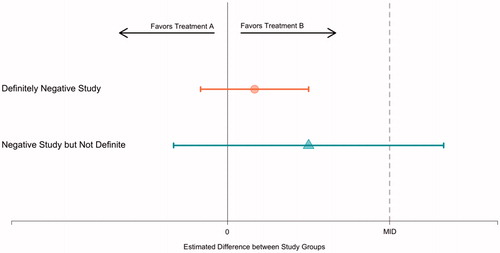
Figure 2 depicts a point estimate and confidence interval for the estimated efficacy. Line 1 of the figure illustrates a definitively negative study. Because the confidence interval includes zero, the result is not statistically significant. Because all the values in the confidence interval are below the minimum important difference, we can confidently interpret the results as negative. As drawn, the confidence interval is narrow, which typically requires a large sample size.

Line 2 of the figure illustrates a study that is not definitively negative. Because the confidence interval includes zero the results is not statistically significant. However, some of the values in the confidence interval are above the minimally important difference, and thus, the confidence interval is consistent with interpretations of both “no difference” and “more than a minimally important difference”. As drawn, the confidence interval is wide, which is typically the result of a small sample size and a correspondingly underpowered study.

How one chooses to describe the results of an underpowered negative study is primarily a question of analytical philosophy and semantics. It is reasonable to say that the results are not statistically significant and then stop. It is similarly reasonable to comment on the direction of “trends”, especially if those trends are clinically plausible, so long as it is clear that what is being described is the direction of the results rather than their statistical significance.

If the analyst chooses to comment on trends, it is important to emphasise the limitations on any conclusions that are tentatively drawn. In particular, while it is true that a larger study should have a narrower confidence interval, that confidence interval would not necessarily be centred on the same value. Indeed, it is possible that the actual effect is zero or otherwise within the portion of the confidence interval that is below the minimum important difference. It is also important to emphasise that p > 0.05 is most properly interpreted as “lacking statistical significance” rather than “equivalence” or “non-inferiority”.

In passing, readers are encouraged not to take statements such as “the trial has 80% power” at face value. Power calculations typically specify their assumptions (and, if not, these assumptions can usually be approximately derived). In fact, what is typically being communicated is something such as “assuming a particular magnitude of efficacy (sometimes termed an “effect size”) and sample size the power is 80%”. It is important to compare the effect size with the minimum important difference. Small studies are usually only powered to detect very large effect sizes – for example, 80% of patients in the intervention group having a good outcome in comparison with 50% in the control group. If less extreme effect sizes are also important, then the power calculation is technically accurate yet potentially misleading.

Underpowered studies are not ideal and, indeed, whether or not it is ethical to intentionally perform them except in special cases (e.g., rare disease with explicit plans for including the results with those of similar trials in a meta-analysis, early-phase trials that are adequately powered for a purpose other than a randomised comparison between treatments, secondary outcomes for a trial that is powered for a primary outcome) is a subject of debate (e.g., [2]).

Discussion

In summary, our proposed answers to the two questions in the introduction are as follows:

1. When a randomised trial has a balanced distribution of covariates, the adjusted and unadjusted analyses should yield similar point estimates of efficacy. If the control variables are strong predictors of outcome, an adjusted analysis should be more precise. Both adjusted and unadjusted analyses are statistically reasonable. The decision should be specified in the analysis plan ahead of time and then followed. When a randomised trial has an unbalanced distribution of an important covariate an adjusted analysis should probably be the default.

2. Whether to consider the direction of effects that are not statistically significant is a question of analytical philosophy. There is nothing inherently wrong about doing this, so long as the lack of statistical significance is appropriately cited.

Disclosure statement

No potential conflict of interest was reported by the authors.

References

- Hauck WW, Anderson S, Marcus SM. (1998). Should we adjust for covariates in nonlinear regression analysis of randomized trials? Control Clin Trial 19:249–56.
- Halpern SD, Karlawish JHT, Berlin JA. (2002). The continuing unethical conduct of underpowered clinical trials. JAMA 288:358–62.