Regional deep hyperthermia: quantitative evaluation of predicted and direct measured temperature distributions in patients with high-risk extremity soft-tissue sarcoma

Abstract

Background: Temperature distributions resulting from hyperthermia treatment of patients with high-risk soft-tissue sarcoma (STS) were quantitatively evaluated and globally compared with thermal simulations performed by a treatment planning system. The aim was to test whether the treatment planning system was able to predict correct temperature distributions.

Methods: Five patients underwent computed tomography (CT) fluoroscopy-guided placement of tumor catheters used for the interstitial temperature measurements. For the simulations, five 3 D patient models were reconstructed by segmenting the patient CT datasets into different tissues. The measured and simulated data were evaluated by calculating the temperature change ($\Delta \mathrm{T}$), T90, T50, T20, T_mean, T_min and T_max, as well as the 90th percentile thermal dose (CEM43T90). In order to measure the agreement between both methods quantitatively, the Bland–Altman analysis was applied.

Results: The absolute difference between measured and simulated temperatures were found to be 2°, 6°, 1°, 4°, 5° and 4 °C on average for T_min, T_max, T90, T50, T20 and T_mean, respectively. Furthermore, the thermal simulations exhibited relatively higher thermal dose compared to those that were measured. Finally, the results of the Bland–Altman analysis showed that the mean difference between both methods was above 2 °C which is considered to be clinically unacceptable.

Conclusion: Given the current practical limitations on resolution of calculation grid, tissue properties, and perfusion information, the software SigmaHyperPlan™ is incapable to produce thermal simulations with sufficient correlation to typically heterogeneous tissue temperatures to be useful for clinical treatment planning.

Keywords:

• Invasive thermometry
• thermal simulation
• regional deep hyperthermia
• thermal dose
• Bland–Altman analysis

Introduction

Regional hyperthermia (RHT) is considered a well-established, nonablative technique that is of clinical value, only when combined with radiotherapy and/or chemotherapy. The clinical effectiveness of the RHT was proven in several randomized clinical trials with various advanced tumors, including sarcoma, melanoma, head and neck, recurrent breast cancer, cervical cancer and bladder cancer [1–4]. Elevated temperatures in the range of 40–43 °C inside the tumor volume together with an improved temperature control are essential for good clinical response, whereby excessive heating of normal tissues should be prevented [5]. Treatment outcomes, such as tumor regression and normal tissue effects, depends on achieved temperature [6,7]; and a thermal dose of 43 °C for 1 h is generally considered optimal [8].

One of the most common established approaches to control and monitor the tumor temperature during tissue heating, is the clinical use of minimally invasive or invasive thermometry. To this end, closed-tip catheters are used, in which temperature sensors, so-called Bowman thermistors, were inserted in order to read the temperatures along the catheter tracks. These catheters are placed either directly in the treated tumor region, (invasive) or in hollow organs close to the tumor volume (minimally-invasive), such as the rectum, vagina and bladder. The minimal-invasive thermometry in the pelvic tumors was as effective as invasive thermal monitoring [9]. The use of invasive catheters in the tumor is relatively time-consuming and can be associated with potential risks such as hemorrhages, infections, acute side effects, and a low acceptance by patients and physicians [10]. Nonetheless, many clinical studies reported that interstitially measured temperatures correlate well with clinical endpoints [11,12]. However, thermometry using these types of temperature thermistors is normally restricted to selected sites of the tumor or the normal tissues [13]. An alternative approach is magnetic resonance (MR)-based thermometry which offers the opportunity for noninvasive 3 D thermometry by collecting temperature information throughout the patient body including regions where no catheters are inserted [5]. However, the reliability of the magnetic resonance imaging (MRI)-based thermometry, in particular in the pelvic and abdominal region, is generally affected by patient, and organ motion as well as blood flow [14].

Hyperthermia treatment planning (HTP) can be a very useful instrument to gain accurate information about the 3 D temperature distribution in the patient, as well as to optimize hyperthermia treatments. With the HTP specific absorption rate (SAR), and temperature distributions can be estimated in the patient using numeric calculations [15]. In addition to that, numerical optimization approaches can be employed to predict phase-amplitude settings which yield appropriate tumor tissue heating [16–18]. The accuracy of pretreatment planning is highly dependent on dielectric and thermal tissue properties, which are usually taken from literature and feature a large deviation [19,20], yielding significant quantitative uncertainties in temperature predictions [20–22]. For clinical application, Kok et al showed in recent studies that HTP can even be applied on-line during hyperthermia treatment in order to improve tumor temperatures in a real-time setting [21,22].

There are some research and commercial software packages available in several clinical centers which can be used for HTP [21,23]. However, for the use in clinical hyperthermia applications, there is a necessity to validate, by utilizing planning systems, especially with respect to its accuracy for patient-specific predictions as well as its robustness. The most widely utilized commercial HTP software is SigmaHyperPlan^TM (Dr. Sennewald Medizintechnik GmbH, Munich Germany), was specifically designed for RHT and was employed in this study for all thermal simulations. This has been clinically validated by comparing simulations with real measurements of specific absorption rate (SAR) distribution, which is measured either in phantom or within the patient in so-called tumor-related reference points [24,25].

Currently, there is no study in the literature investigating the comparison between interstitial and simulated temperature distributions in sarcoma patients using the SigmaHyperPlan^TM. Therefore, the aim of this study was firstly to quantitatively analyze clinical data collected by the invasive thermometry of patients with high-risk soft-tissue sarcoma (STS) located in the lower extremity region. In the second step, the accuracy of the HTP was evaluated by comparing interstitial temperature data with the simulated data. Here, it must be emphasized that the ultimate goal of our data evaluation was to test whether the SigmaHyperPlan^TM is able to predict correct temperatures like those measured by invasive thermometry. The outcome of this study will allow us to answer the question, whether the SigmaHyperPlan^TM can be reliably utilized for thermal simulations of the STS patients, where the tumors are located laterally.

Methods

Invasive thermometry

Patient data acquisition

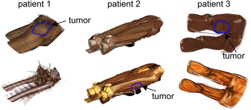
The analysis presented in this study covered five patients with STS in the upper leg region (Table 1). CT scanning of each patient was performed for HTP using a Somatom Sensation Open (Siemens Healthineers, Erlangen, Germany) CT system. The patients were positioned head first, supine with arms up (similar to the hyperthermia treatment position). The CT field of view (FOV) was approximately 60 cm ± 5 cm to cover the entire hyperthermia applicator. The CT scan parameters were 512 × 512 acquisition matrix; 4 mm ± 1.4 mm slice thickness, 120 kV tube voltage and 150 mA tube current. The in-plane resolution of the reconstructed CT images was 1 × 1 mm². No contrast agent was administered during the CT scan. Following the data acquisition, a radiologist determined the hyperthermia gross tumor volume (HT-GTV) from the CT (or sometimes MR images) before the beginning of treatment. The radiologist treatment plan was used for the entire course of hyperthermia patient treatment.

Table 1. Patient characteristic, including the number of the CT slices used for manual and semi-automatic segmentation of structures.

Patient	Gender	Diagnosis	# of CT slices	# of catheters	Tumor volume/cm³
1	m	leiomyosarcoma	178	3	511
2	f	rhabodomysarcoma	120	2	290
3	f	pleomorphic sarcoma	100	2	226
4	m	Synovial sarcoma	191	1	501
5	m	pleomorphic sarcoma	131	2	188

Implementation of tumor catheters

All consecutive patients, from February 2016 to May 2017, underwent CT fluoroscopy-guided closed-tip polyethylene catheter implementation for RHT. All patients, who were assigned to the closed-tip catheter placement, had high-risk STS (size >5 cm, histological grade 2 or 3) and were scheduled for neoadjuvant chemotherapy with RHT. The patients underwent pre- and post-interventional CT imaging. Multiplanar reconstructions were utilized to obtain the extent of the tumor. Furthermore, the reconstructions were employed to detect the neighboring anatomical structures and to plan the ideal needle position for catheter placement. For the CT guidance, a 128-slice CT system with CT fluoroscopy (CARE Vision CT, Siemens; 120 kV, 10–20 mA) was used. CT fluoroscopy was driven with angular beam modulation (HandCARETM, Siemens). The whole catheter implementation was performed under periodical single-shot CT fluoroscopic acquisitions only. Further details about the CT fluoroscopy in RHT are described by Strobl et al [10]. The procedure of the catheter invasive placement was carried out by a board-certified radiologist with an experience of over 5 years in CT-guided interventions. The patient position and access route was normally chosen based on the localization of the tumor. The catheters were placed at the same distance from each other, especially when more than one was used. When tumors had both necrotic and solid parts, where possible, the catheters were positioned in the solid region. The insertion was then halted when the needle covered as much as possible of the tumor diameter. Thereafter, a control CT scan was made to ensure that there was no active bleeding or other complications and also to verify a correct position of the tumor catheters. These catheters were placed one day before the start of the hyperthermia treatment and remained for two treatments in the tumor, and they were removed immediately after the second hyperthermia treatment. Figure 1 shows the 3 D volume rendering of the tumor catheters of three exemplary patients.

Figure 1. 3D volume rendering of three exemplary STS patients with implemented catheters in the tumor.

Hyperthermia treatment

The patients were treated inside the SIGMA-Eye applicator (BSD-2000/3D, Pyrexar Medical Corp., Salt Lake City, UT). The central point of the HT-GTV of each patient was placed at the central plane of the applicator. The thermometry data were collected from the first patient treatment. All channels of the applicator were set to 100% of the applied power (Table 2). The maximum power was determined patient-specific at the first treatment day. The maximum power was adjusted by considering desired temperature range (40–43 °C) in the tumor, patient feedback regarding complaints and superficial sensation at the patient skin surface. The target focus for each patient was determined from the 2 D CT coordinates (x_CT,y_CT) of the HT-GTV center. The hyperthermia coordinates (x_HT,y_HT) were then calculated theoretically, which is based on many focus measurements with our lamp phantom (width = 380 mm, height = 255 mm) inside Sigma 60, Sigma-Eye and Sigma-Eye MR applicators. It turns out from these phantom measurements that the clinically useful range of the focus adjustment in the X-axis is from −7 to 7 cm and in the Y-axis from −4 to 4 cm. The hyperthermia focus is calculated using the following formula: $$(X_{\mathit{HT}},Y_{\mathit{HT}})=\left[\frac{X_{\mathit{CT}}}{\raisebox{1ex}{$380$}\!\left/ \!\raisebox{-1ex}{$2$}\right.}\mathrm{\times }7,\frac{Y_{\mathit{CT}}}{\raisebox{1ex}{$255$}\!\left/ \!\raisebox{-1ex}{$2$}\right.}\mathrm{\times }4\right]$$

Table 2. Applicator setting for both patient treatments and thermal simulations.

Patient	Focus (x,y)/cm			power/watt
	Treatment	HTP_I	HTP_II	Treatment	HTP_I	HTP_II
1	(6,2)	(0,0)	(0,0)	730	613	730
2	(4,0)	(0,−3)	(0,−3)	521	451	521
3	(−3,−1)	(−4,−2)	(−4,−2)	336	334	336
4	(−5,1)	(−8,2)	(−8,2)	440	696	440
5	(−5,5)	(−5,1)	(−5,1)	420	604	420

The Bowman thermistors with an accuracy of ±0.2 °C were inserted to the tip of the tumor catheters. These thermistors are transparent for the electromagnetic field, due to their high resistance of the carbide wires. For the temperature reading, a clinical thermometry system was employed, consisting of stepping motors which ensured that the thermistors could be pulled out in 5–10 mm increments up to maximum mapping length of 200 mm through the catheter in tumor. Temperatures were continuously recorded within a time interval of 6 min during the RHT. Due to the fact that temperature distribution in tissues during electromagnetic radiation is not uniform, it is important to monitor temperatures not only in the HT-GTV, but also in the surrounding anatomical structures. This has not been considered in this study due to absence of invasive catheters in the normal tissues.

Thermal simulations

SIGMA-Eye applicator

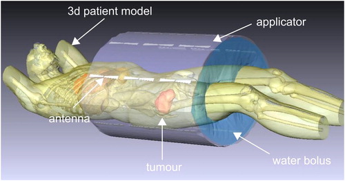
A model of the SIGMA-Eye applicator in the software SigmaHyperPlan^TM, which was used for the electromagnetic (EM) as well as thermal simulations, is shown in Figure 2. The applicator consists of three rings of 24 dipole antenna pairs that are coupled in 12 channels of two antennas each. Amplitudes and phases of the hyperthermia signals, which are fed into each antenna, can be adjusted in order to control the interference of the radio frequency (RF) field [26]. The arrangement of 24 dipole antennas in the SIGMA-Eye allows for 3 D steering capability. A significant improvement in the quality of tumor heating can be achieved with the SIGMA-Eye [27].

Figure 2. Thermal simulation setup in the software SigmaHyperPlanTM.

Patient modeling and EM-simulations

Using the patient CT dataset with a cranial-caudal length of at least 60 cm, a 3 D discrete patient model was reconstructed by manual/semi-automatic segmentation of different tissue structures (Figure 2). For all simulations, five organs (i.e., fat, muscle, bone, bladder and blood vessels) were contoured. In addition to that, the HT-GTV was delineated covering the target volume. The challenge in this study was to segment the catheters, since each patient underwent two CT scans collecting two datasets. The first dataset acquired with large CT-FOV before the catheter placement, whereas the second dataset collected with small FOV, restricted to the longitudinal catheter length. In both acquired CT datasets, the patient positions were different. The first step was to perform a rigid image registration using the open-source software elastix [28], in order to match the patient position in both CT data sets. After that, the catheters were manually delineated and added to the segmentation of organs. Then, a 3 D patient model was generated from the segmented structures. Further details on the workflow for the 3 D modeling of the patient are described by Gellermann et al and Aklan et al [24,29]. On average, the patient models consisted of 70 800 tetrahedra, ±19 000 nodes, and 150 700 triangles with edge lengths of the tetrahedral between 6 and 28 mm, with the dense grid mostly in regions with high tissue contrasts and near the antennas. These numbers were predefined in the SigmaHyperPlan^TM manual to generate the 3 D patient grid model. Furthermore, other studies employed similar numbers of tetrahedral [25,29,30], and support our simulation setting.

The antenna model implemented in the planning system corresponded to the SIGMA-Eye applicator of the BSD-2000 system for the regional hyperthermia. The biconical dipole antennas of the applicator were modeled by pairs of metallic cones (Figure 2), with certain estimates about the neighboring medium in the feeding point as well as around the antennas. After successful generation of the patient model, the grid was extended to incorporate the applicator (antennas and water bolus) and the surrounding air. The selected applicator was automatically aligned with the patient model, whereby the tumor center was aligned in the central plane of the applicator. A water bolus grid (grid size 25 mm) for the SIGMA-Eye, considering the realistic inside bended surface, was then adapted to the positioned patient model with a grid resolution of 10 mm. The bolus was then refilled with tetrahedrons, and the grid for the surrounding air (grid size 50 mm) was generated. EM cross-coupling between antennas was to some extent considered in the software SigmaHyperPlan^TM according to its manual.

The finite element (FE) method was utilized for all EM simulations. The SAR distribution for each point in the patient model can be obtained by superposition of the EM fields of all applicator antennas using the solver of SEMCAD-X (SPAEG, Zurich, Switzerland). The temperature distribution can then be predicted using the thermal tissue properties defined in the database of the HTP software [29]. The simulation of the temperature distribution was determined in the steady state by solving the bioheat-transfer equation on the same grid. The body temperature for all calculations was set to 37 °C and the bolus temperature to 25 °C. Through an optimization process of amplitudes and phases of the 12-applicator antenna pairs surrounding the patient, a focus of the temperature in a predefined target volume can be achieved, while keeping the healthy tissues within a tolerable temperature range. More details about the optimization process used in the SigmaHyperPlan^TM are described by Sreenivasa et al and Canters et al [25,31].

Two different treatment plans of each patient model were created to adjust the amplitudes and phases of the applicator in the simulation:

1. HTP_I: Amplitudes and phases were fully optimized by the HTP.

2. HTP_II: Amplitudes were set manually to 100% after the optimization similar to the real patient treatment, while the phases were left optimized. The optimized power was adapted to the power used in the patient treatment.

Table 2 summarizes the applicator parameters that were utilized in both simulations and real patient treatments.

Lamp phantom measurements

The electrical field distributions were measured in an elliptical lamp phantom by applying the three treatment plans for each patient, namely HTP_I, HTP_II and the plan of the real patient treatment. The phantom has dimensions of 38 × 22 cm (long axis, short axis) with a fat-equivalent phantom shell of 1 cm thickness (ε_r = 10, σ = 0.04 S/m). The length of the phantom is 100 cm in total with a 50 × 37 cm rectangular opening at its back end. The closed front part of the phantom is 50 cm long. The phantom has an elliptical base plate with array of approximately 342 electrical field-sensitive lamps [32].

The phantom was filled with conductive water and positioned in the applicator with the base plate placed at the center of the SIGMA-Eye applicator, where the electric field is highest. For all phantom measurements, lower power of 400 watts was applied to avoid destroying the lamps. 2 D Photograph images were then shot for each applied plan.

Data analysis

Treatment temperature data

The single steps of the evaluation process of both interstitial and simulated temperature data is presented in Figure 3. It must be emphasized that all interstitially measured temperature data were first collected during the patient treatments and then compared afterwards to the simulated temperatures. The patient temperature data obtained from the Bowman thermistors were analyzed with in-house developed C++ code combined with R (The R Foundation for Statistical Computing, Vienna, Austria) [33]. The temperatures T90, T50 and T20 as well as the cumulative equivalent minutes at 43 °C for the T90 temperature (CEM43T90), which is used as measure for the thermal dose applied, were calculated. The CEM43T90 is the 10^th percentile dose – the thermal dose that 90% of the rest of measured thermal doses exceed. It is 10% above the minimum thermal dose. Additionally, T_mean, T_min and T_max were also determined. Beyond that, the temperature rise ($\Delta \mathrm{T}$) for the 90^th percentile temperature (T90) above normal body temperature (37 °C) was calculated as: $$\Delta \mathrm{T}=\mathrm{T}90-37°\mathrm{C}$$

Figure 3. Flowchart illustrating the evaluation procedure of both treatment and simulated temperature data.

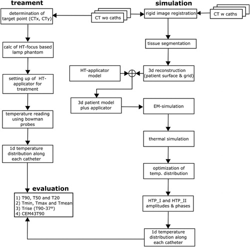
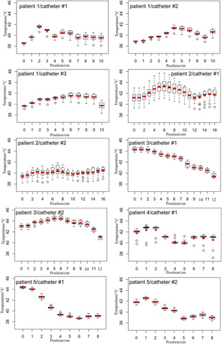
The acquired thermal distribution of each tumor catheter for each patient was visualized in the form of a box plot as a function of distance. Furthermore, the calculated index temperatures were averaged for each catheter within the therapeutic treatment time (from 30 min until 90 min) and illustrated as a boxplot, which represented the time-averaged temperature values for all mapping positions of the catheter. In order to be able to compare the simulation to the real patient treatment, the index temperatures in Figure 4 were averaged within the steady-state treatment time, at which the temperatures in the thermal simulations were in principle calculated.

Figure 4. Measured temperatures along the tumor catheters for all treated patients. Note that the height of each boxplot represents the measured values over the entire treatment time for each catheter position. The red points are the calculated mean values and the black bold line in the boxplot gives the median value. The position 0 cm means that the sensor was located at the catheter tip. The temperature mapping was in 1 cm steps.

Simulation temperature data

To evaluate the simulated data in the same manner as the measured data, only the simulated temperature values along the tumor catheter were obtained by applying a mask consisting of only the segmented catheters to the 3 D simulated thermal maps of the patient model. The T90, T50, T20, T_min, T_max and T_mean were determined using MATLAB 2012 b a (MathWorks, Inc., Natick, Massachusetts, US). The difference of the index temperatures between simulation and real patient treatment (within the steady state treatment time) was determined using the following formula: $$\Delta (°C)=\left|T_{\mathit{treament}}-T_{\mathit{simulation}}\right|$$

Moreover, the $\Delta \mathrm{T}$ of the simulated temperatures and its difference were also computed, where the treatment data was taken as a reference.

For better measuring the agreement between both methods, Bland–Altman [34] plots of the temperature were created using temperature data from all patients. The Bland–Altman approach includes plotting differences between the results of both approaches as a function of averages between them. Such representation is visually more informative than calculating the relative difference. The average ($m$) and standard deviation ($\sigma$) of the differences between two methods were determined. The values of $m+2\sigma$ and $m-2\sigma$ were calculated in the confidence interval of 95%. In accordance with the suggestion of Bland and Altman and of clinical reasoning, differences beyond $m\pm 2\sigma$ could be judged clinically important. These values are used to make a decision on whether the differences between the interstitial and simulation temperature data are important and if they are not, then both methods may be used interchangeably.

Results

The results of the invasive thermometry of the five patients indicated different temperature distributions along the tumor catheters, as shown in Figures 4 and 5. The heating of the sarcoma tumor tissues showed inhomogeneous distributions apart from the tumor volume and location.

Figure 5. Calculated temperatures using the data from Figure 1. Note that the width of the boxplot reflects the time-averaged temperature values for all mapping positions. The red point is the computed mean value.

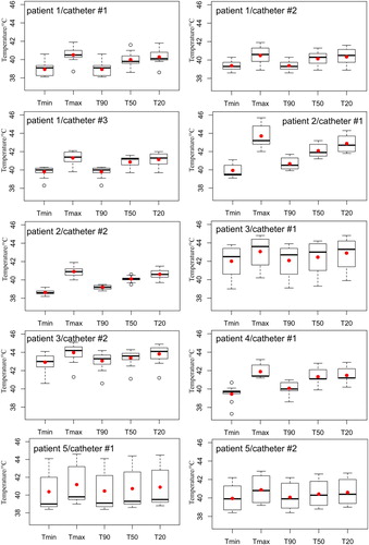
Considering the temperature distribution of the first patient, the temperatures at the tumor margin were significantly lower than those observed in the catheter position of 3–9 cm, as shown in Figure 4. After reviewing the patient CT images, it was seen that a relatively large blood vessel was located close to the tip of the tumor catheters. The temperatures of the tumor tissues with probably less or even no blood circulation were substantially higher than at the tumor rim. Therefore, the CEM43T90 of this treatment was found to be low, as reported in Table 3. Although the power applied (730 watts) for this patient treatment was considered be higher compared to other patient treatments. A similar observation was seen in the temperature data of the second patient. The thermometry showed heterogeneous temperatures in both tumor catheters, where catheter #1 exhibited higher temperatures above 44 °C than catheter #2, as illustrated in Figure 5. Conversely, the third patient’s treatment featured essentially a higher thermal dose with a lower power of 336 watts, measuring higher temperatures due to the large amount of liquid inside the tumor. From that, it can be stated that aqueous parts of the tumor in RHT are fast to heat. This was clearly seen during the treatment, whereby the therapeutic temperature of 43 °C was reached in the first five minutes of the heating process. Furthermore, the temperature during the transition between tumor and muscle tissues dropped down to approximately 40 °C from 44 °C in the catheter position of 10–12 cm. The thermal dose of this patient treatment was also significantly high.

Table 3. Thermal dose (CEM43T90) values for both patient treatments and thermal simulations.

	Patient 1			Patient 2		Patient 3		Patient 4		Patient 5
	Catheter
	1	2	3	1	2	1	2	1	1		2
HTP_I	3.8	3.8	0.9	0.2	0.2	0.2	0.9	0.9	15		0.9
HTP_II	3.8	0.9	0.2	0.2	0.2	60	3.8	0.2	3.8		3.8
Treatment	0.2	0.3	0.6	2.9	0.3	30	55	1.4	0.1		0.2

The fourth patient showed temperature fluctuation along the tumor catheter. The tumor of this patient was less perfused and hence clear temperature gradients were seen with thermal dose of 1.5 min. The last patient, however, showed an interesting temperature behavior, when the sensor passed over the tumor, in the catheter position of 0–2 cm, into the muscular tissues in the distance from 3 to 8 cm. The measured temperature inside the tumor was around 42 °C and was about 39 °C inside the muscles. The thermal dose was almost similar to the first patient treatment due to the effect of the blood perfusion. The temperature change ($\Delta \mathrm{T}$) was on average 3 °C in all patients, except in the third patient where a higher temperature increase of nearly 5 °C was observed, as listed in Table 4.

Table 4. Temperature change ($\Delta \mathrm{T}$) of T90 above the patient body temperature of 37 °C.

	Patient 1			Patient 2			Patient 3		Patient 4		Patient 5
	Catheter
	1	2	3		1	2	1	2	1	1		2
HTP_I	4	4	3		2	2	2	3	3	5		3
HTP_II	4	3	2		2	2	6	4	2	4		4
Treatment	2	2	3		3	2	5	6	3	3		3

On the other hand, the thermal simulations showed a considerable variability in the temperature predictions as well as in the calculated thermal dose, as reported in Tables 3, 4, 5 and 6. It can be noticed that predicted temperatures up to 49 °C were observed among the simulation results. The 3 D simulated thermal maps, overlaid on the anatomical coronal CT image, commonly feature inhomogeneous distribution across the 3 D modeled patients, as presented in Figure 6. Furthermore, the thermal maps of patients 1, 2, 3 and 4 show a slight temperature increase in the healthy tissues, which might be interpreted as critical hot spots. This may have potentially occurred because of the location of the tumors to the high-density bone structures, leading to higher reflection and/or absorption of the electromagnetic waves. Such details about the development of hot spots in the healthy tissues were not feasible with the data of invasive thermometry due to the restriction of the number of placed catheters. The simulations of the HPT_II (Table 6), where the power amplitudes of the modeled applicator were kept similar to the patient treatments, did not significantly differ to the results of the HTP_I (Table 5). The absolute difference between measured and simulated temperatures were found to be 2°, 6°, 1°, 4°, 5° and 4 °C on average (Tables 7 and 8) for T_min, T_max, T90, T50, T20 and T_mean, respectively. A smaller temperature difference in the T90 was seen. Moreover, the difference in the temperature change of T90 showed deviation in the range of 1° to 4 °C from the measured temperatures as shown in Table 9.

Figure 6. Coronal cross-sections thermal maps, overlaid on CT images, of the five STS patients generated from the HTP_I. The maps show relative inhomogeneous temperature distributions within the HT-GTV. Note that some hot spots are developed either within the muscle tissue or close to the bone.

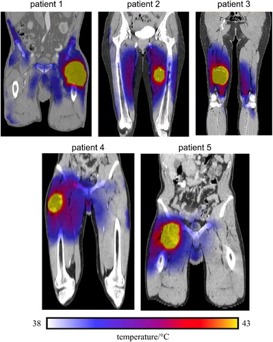
Table 5. Temperatures obtained from the HTP_I. Note that the core body temperature is 37 °C.

	Patient 1			Patient 2			Patient 3		Patient 4		Patient 5
	Catheter
	1	2	3		1	2	1	2	1	1		2
Tmin	38	39	37		37	37	40	38	38	38		37
Tmax	45	48	48		48	48	46	43	49	48		48
T90	41	41	40		39	39	39	40	40	42		40
T50	44	46	45		44	44	43	41	46	47		48
T20	44	48	47		47	47	45	42	48	48		48
Tmean	43	45	45		43	43	43	42	45	46		46

Table 6. Temperatures calculated from the thermal simulation HTP_II.

	Patient 1			Patient 2			Patient 3		Patient 4		Patient 5
	Catheter
	1	2	3		1	2	1	2	1	1		2
Tmin	37	38	37		37	37	38	39	40	37		37
Tmax	46	47	46		48	47	49	49	47	48		48
T90	41	40	39		39	39	43	41	39	41		41
T50	44	44	43		46	43	47	46	44	46		46
T20	45	47	44		47	45	48	48	45	48		47
Tmean	44	44	42		45	42	46	46	43	45		45

Table 7. Temperature differences between patient treatment and thermal simulation HTP_I.

	Patient 1			Patient 2			Patient 3		Patient 4		Patient 5
	$\Delta \mathrm{ }(°\mathrm{C})$
	Catheter
	1	2	3		1	2	1	2	1	1		2
Tmin	1	0	3		3	1	2	5	1	2		3
Tmax	4	8	7		5	8	3	1	7	7		7
T90	2	2	0		1	1	3	3	0	2		0
T50	4	6	4		2	5	1	2	5	6		8
T20	4	8	6		5	7	3	2	7	7		7
Tmean	3	5	4		2	4	1	1	4	5		6

Table 8. Temperature differences between patient treatment and thermal simulation HTP_II.

	Patient 1			Patient 2			Patient 3		Patient 4		Patient 5
	$\Delta \mathrm{ }(°\mathrm{C})$
	Catheter
	1	2	3		1	2	1	2	1	1		2
Tmin	2	2	2		3	1	4	6	2	3		3
Tmax	5	7	5		5	7	6	5	5	7		7
T90	2	1	1		1	1	1	2	1	1		1
T50	4	4	2		4	4	5	3	3	5		6
T20	5	7	3		5	5	6	5	4	7		6
Tmean	4	4	1		4	3	4	3	2	4		5

Table 9. Differences of $\Delta \mathrm{T}$ for both thermal simulations, where the patient treatment served as a reference.

	Patient 1			Patient 2			Patient 3		Patient 4		Patient 5
	$\Delta (°\mathrm{C})$
	Catheter
	1	2	3		1	2	1	2	1	1		2
HPT_I	4	4	3		2	2	2	3	3	5		3
HTP_II	4	3	2		2	2	6	4	2	4		4

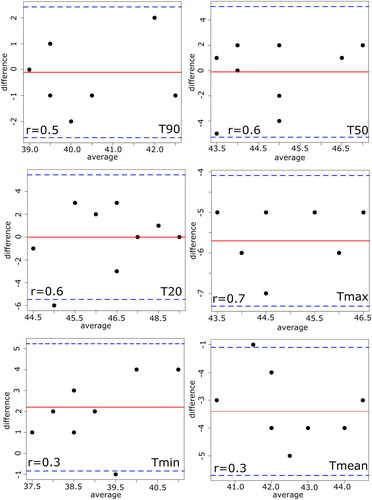
Figure 7 uncovers the fundamental difference between patient treatments and thermal simulations, where the electrical field distributions of all three plans were measured using the lamp phantom. The phantom measurements were performed inside the SIGMA-Eye applicator with a power application of 400 watts. The results indicated that the distributions of both thermal simulations drifted significantly in their distribution form as well as the position of hot spot, when they are compared to those of the real patient treatments. Furthermore, the measured focuses of the thermal simulations were found to have a large divergence to those of patient treatments. In order to measure the agreement between both methods quantitatively, the Bland-Altman method was applied by calculating the differences and averages of the temperatures. Figures 8 and 9 show the results of the Bland–Altman quantitative analysis where the mean of the differences lay between −5° and 2 °C for HTP_I and between −.4° and 0.1 °C for HTP_II. In addition, the correlation coefficients between both approaches seem to be poor in all temperatures (Figure 7). While the standard deviation of the differences is in the range of 1° to 3 °C for both thermal simulations, the lower confidence limits $m-2\sigma$ ranged from −1° to −11 °C and the upper confidence limits $m+2\sigma$ from −2° to 5 °C for HTP_I. For the HTP_II, the corresponding results of $m-2\sigma$ was between −1° and −11 °C and of $m+2\sigma$ it was in the range of −2° and 5 °C. In general, the HTP_I featured larger differences than HTP_II.

Figure 7. 2D Photograph images of the lamp phantom positioned inside the SIGMA-Eye applicator, where the applicator settings of patient treatment, HTP_I and HTP_II were applied. The hot spot in the phantom presents the 2D electrical field distributions using 400 watts for all phantom measurements. Note that the field distributions of HPT_I and HTP_II feature a significant deviation with respect to the shape of the distribution and the hot spot position, when they compared to the treatment settings.

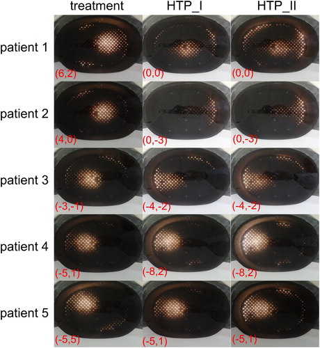
Figure 8. Bland–Altman plot with the corresponding correlation coefficient (r) between the real patient treatment and thermal simulation HTP_I. The solid line shows the mean $m$ of differences between both methods and the thin dashed lines show $m\pm 2\sigma$ of confidence interval of 95%, where $\sigma$ the standard deviation of the differences. Note that values with the same differences will be plotted on the top of each other.

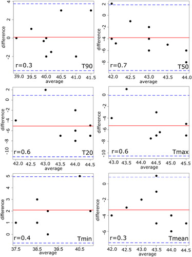
Figure 9. Bland–Altman plot with the corresponding correlation coefficient (r) between the real patient treatment and thermal simulation HTP_II.

Discussion

This study demonstrated a global comparison between invasive thermometry and thermal simulations. The evaluation was performed using five high-risk STS patients with catheters placed in the tumor. The software SigmaHyperPlan^TM was utilized for the thermal simulations. The accuracy of the SigmaHyperPlan™ modeling with measurements has been systematically investigated in previous studies [24,25]. Gellermann et al assessed the clinical practicability and accuracy of the planning software, and found that the bias between the absolute measured and simulated SAR was ±20%. Sreenivasa et al. verified the software by including 30 patients with cervical, rectal and prostate cancers and showed a good correlation between model calculations and clinical data regarding the temperature distribution in these tumors [25]. She concluded that the software delivers valuable information, not only for pre- and clinical practice, but also for further technological improvements. In our study, the accuracy of the SigmaHyperPlan™ was evaluated with direct measured temperatures inside the HT-GTV using clinical data of five STS patients.

In spite of using a very limited number of tumor catheters in each patient, the invasive thermometry provided important clinical details about the tumor behavior with different types of sarcoma tumors. The results showed that the temperature increase inside the tumors is generally dependent on following factors: (1) Anatomical heterogeneity within the tumor tissues resulting into different dielectric properties; (2) Inter- and intratissue tumor perfusion under thermal stress conditions; (3) Location of blood vessels related to the tumor volume. The lower temperatures observed at the tumor margin (Figure 4 in patients 1 and 2) compared to the tumor center are probably caused by a decrease of the blood perfusion due to the adjacent hyperperfused muscle, the so-called steal-effect [14]. However, temperatures were substantially higher in regions of low or negligible perfusion, such as in necrotic tumor. Increased perfusion in the muscle tissues induced a reduction of the measured temperature during RHT, as seen in patient 3 (Figure 7). Blood perfusion works as cooling mechanisms in addition to thermal conduction and water bolus cooling, which are not taken into account in the HTP and may have a large effect on the temperature. The sarcoma tumors usually have very heterogeneous and chaotic vessel networks with various perfusion changes leading to heterogeneous temperature distributions. Perfusion measurements using the MRI technique could be very useful to monitor the perfusion effects during the RHT treatments [13,14]. Further, the sarcoma tumors with a relative large amount of watery collection quickly reached the therapeutic temperature (Figure 4, patient 3). Such watery collections feature higher electrical conductivity as well as lower perfusion in comparison to the solid parts of the sarcoma tumor resulting in a relative rapid heating-up.

The results of the thermal dose CEM43T90 (Table 3) of all patients, except patient 3, show that the values are quite low (0.2–3 min) within the tumor catheters. In patient 3, however, the CEM43T903 was higher and found to be 29–55 min, despite a relative low applied power. This is an indication that tissue properties of the tumor have a significant impact on the thermal response to the RF energies. For instance, the tumor of patient 3 featured a relative high liquid fraction, which was observed during both CT imaging and catheter implementation. The tumor appeared to progress during RHT therapy, and a surgical procedure was performed prematurely. The result of the pathological analysis showed a pseudo-progression due to a volume increase caused by enclosed bleeding. Furthermore, extensive necrosis (>90%) was found. Interestingly, the pathological response (tumor necrosis rate >90%) showed a significant correlation with CEM43T90 in the tumor volume. On the other hand, smaller CEM43T90 values in non-responders were likely associated with a higher tumor perfusion rate and consequently lower temperatures. In patient 1, neoadjuvant chemotherapy was planned followed by pathologic assessment, which revealed a central necrotic component of 20–30%. However, in order to make a clear statement about the correlation between CEM43T90 and necrosis in the tumor in this study, all patient treatments from the start of the therapy to the time of surgery should be considered, which is beyond the scope of this study.

The interstitial temperature measurements could be influenced by the thermal mapping system which provides only a limited spatial temperature resolution. It has the drawback that only temperature data will be successively acquired at a predetermined distance, so that no data can be acquired during the movement phase of the thermistors. Moreover, the thermal mapping device is a mechanical system consisting of a rotary motor, which in turn has a measuring uncertainty and thus inaccurate position reproducibility. This would restrict the measuring precision of the temperature measurements. Furthermore, the simulation and the measured temperatures were compared only as distribution and not at individual points along each catheter due to the large tetrahedron dimensions used in the calculation grid. Additionally, the invasive tumor catheters have a limitation in measuring hot spots outside the HT-GTV, which normally occur at the surface of two different tissue structures. The evaluation of the occurrence and behavior of possible hot spots was neglected in this study due to the absence of the invasive catheters in the normal tissues, which was clinically not feasible. Moreover, location of these invasive catheters could be changed from the implantation day until the first hyperthermia treatment, as these catheters were fixed using filaments attached to the patient skin. Such catheter misalignments could happen during the patient sleep phase and movement, or even when the tumor is predominantly composed of fluid tissue (e.g., patient 3). This effect would clearly impact the results of this study, since the position of the catheters was taken from the CT dataset directly after the implementation. The initial CT position of the catheter could not be ensured at the day of the hyperthermia treatment, in most of the clinical cases. A new CT scan to verify the correct catheter positions was not possible in the clinical routine.

The thermal simulations exhibited overall higher predicted temperatures than the invasive thermometry. Particularly questionable temperatures were those that were higher than 45 °C. Moreover, the temperature rise of simulated temperatures was substantially higher than those observed during the real patient treatments (Table 4). The deviation between thermal simulations and real patient treatments was in the range of 2 °C lower and 6 °C higher (Figures 8 and 9, Tables 7 and 8). The observed difference is clinically not acceptable and thus both approaches should not be used interchangeably. Nevertheless, the results of the invasive thermometry revealed important observations that help to practically improve the accuracy of the HTP, although few catheters were placed in the tumor. These could largely enhance the accuracy of thermal simulations with the SigmaHyperPlan™. One of these observations is inter- and intratissue tumor perfusion under thermal stress conditions. Heat exchange between blood vessels and tissue strongly depends on the flow rate, which can increase considerably during RHT [35] depending on the local temperature rise and the physical condition of the patient. To this end, a temperature dependent perfusion model instead of using a global value for the blood circulation, which is the case in the SigmaHyperPlan™, might be helpful to further improve the temperature predictions [17]. A previous study reported that ignoring the temperature dependence of the perfusion can lead to a clear overestimation of the absolute thermal dose that can be delivered [36]. Therefore, modeling using realistic 3 D vessel networks is important for accurate absolute temperature predictions, since the Pennes model does not take into account the local thermal impact of the vasculature and the direction of the blood flow. One study in the literature tried to implement such an accurate realistic 3 D vessel networks into the HTP system, showing that the feasibility of online temperature-based simulations with such networks will lead to improvement of tumor temperatures [37]. However, further research investigation is required to assess the benefit of such adaptive treatment planning system and whether the possible advantage justifies the extra patient burden and clinical workload. From the results of the invasive thermometry, it can also be observed that an accurate segmentation of the target volume into different compartments is essential, which consider necrotic, solid and liquid tissues. The different segmented tumor tissues should be then assigned to corresponding dielectric properties. This would mimic a realistic tumor composition and help to reduce the difference between both HTP and real patient treatment. The existing dielectric (i.e., permittivity and effective conductivity) and thermal (i.e., blood perfusion, thermal conductivity, heat capacity, density, and metabolic heat generation) tissue properties show a large variability of approximately 50%, but patient-specific tissue properties are not available and, therefore, average literature values are currently utilized for the simulations with the SigmaHyperPlan™ [20,38]. These uncertainties in the tissue properties might explain why the software is not quantitatively reliable. Recent research projects focus of further improvement of the HTP predictions by reconstruction of patient-specific dielectric properties with the help of MR-based dielectric imaging and advanced thermal modeling using temperature-dependent perfusion and discrete vasculature [17,39,40]. The MR-based dielectric imaging will potentially improve the reliability of the SAR predictions, which are also input for thermal simulations.

There are a series of uncertainties in the HTP that might lead to suboptimal treatment settings and thus would add further error to the thermal simulations. One of these uncertainties is the grid resolution of the 3 D patient model. The grid resolution used in this study was 10 mm for the patient model, 25 mm for the water bolus and 50 mm for the air, which could be reduced to potentially improve the temperature predictions. With such rough resolution, structure information may be lost, particularly at the boundaries between the segmented regions, that is, at the tissue interfaces. Finer anatomical details (such as tissue physiology as well as arteries and veins) needed for the perfusion modeling, are strongly affected by a rough resolution and thus EM and thermal simulations would not be expected to be accurate enough [15]. High grid resolution may be expected to improve the accuracy and reliability of the HTP in routine clinical practice. Another uncertainty is the observer variability in delineating the HT-GTV and organs at risk in terms of segmentation accuracy and temperature predictions. The segmentation variations have a statistically significant impact on the temperature coverage of the target in RHT [41]. This might also influence the results of the planning calculations. Another uncertainty is the patient position, since the patient normally lies on a flat table during the CT imaging with their legs elevated. While the applicator model (Figure 2) available in the simulation is optimal, this does not necessarily reflect reality. For example, fine individual adjustments of the real hyperthermia applicator are necessary, which will not be taken into account in the thermal simulations. The use of an optimization method could also induce an uncertainty to the HTP, which aims for higher temperatures inside the tumor volume and lower temperatures in the surrounding healthy tissues. The predicted temperatures might be influenced by the accuracy of those optimization algorithms [18,42,43].

The electrical field distributions of the third patient were to some extent similar inside the lamp phantom (Figure 7) for simulation and treatment. Therefore, the simulation-based treatment plan was applied in the first 30 min of the second real patient treatment, where the temperature data of the invasive thermometry were taken as reference in order to assess the reliability of the HTP. In fact, low temperatures were observed below 40 °C, while the interstitial measurements in the first treatment showed, however, higher temperatures in the tumor above 44 °C for the same treatment time. For this reason, the simulation-based treatment plans of other patients were not applied for the real patient treatments. Since our treatment facility has more than three decades of experience in performing regional and superficial hyperthermia using invasive thermometry in sarcoma tumors, the amplitude steering as well as the power setting for each individual patient is based on our empirical knowledge and clinical long-term experience. A reliable and accurate treatment planning system, which mimics a real hyperthermia patient treatment, would potentially improve the quality of hyperthermia treatment and thus the clinical outcome. While HTP with current limitations on spatial resolution of calculation grid and tissue properties is not able to provide precise patient specific treatment planning, there are other uses for the SigmaHyperPlan™. This planning tool helps us inherently by investigating the impact of metal implants, patient mispositioning, as well as by comparing the relative heating effectiveness of different applicator settings. Furthermore, it is a useful tool for predicting the treatment hot spot locations in order to distinguish between patients who should be easy to heat or difficult to heat.

Finally, all these mentioned uncertainties could be possible sources for the difference between the invasive thermometry and the thermal simulations in this study, which focused on sarcoma tumors in the extremity region. The evaluation in this study had a low number of patients (n = 5). This is due to the fact that invasive thermometry has a very low acceptance rate by hyperthermia patients.

Conclusion

This study demonstrates that the global difference between invasive thermometry and thermal simulations of temperature distributions in sarcoma tumors is large and clinically unacceptable for routine treatment planning. Given the current practical limitations on resolution of calculation grid and tissue properties as well as perfusion information, the software SigmaHyperPlan™ is incapable to produce thermal simulations with sufficient correlation to typically heterogeneous tissue temperatures to be useful for clinical treatment planning.

Disclosure statement

L.H.L. received research and travel support from Dr. Sennewald Medizintechnik. S.A.-R. received travel support and honoraria from Pyrexar and Medtherm. B.A. und B.Z have received travel support from Dr. Sennewald Medizintechnik to present the results of this work on the ESHO conference 2018 in Berlin. All authors declare no competing interests and responsible for the content and writing of the article.

References

- Issels RD, Lindner LH, Verweij J, et al. Neo-adjuvant chemotherapy alone or with regional hyperthermia for localised high-risk soft-tissue sarcoma: a randomised phase 3 multicentre study. Lancet Oncol. 2010;11:561–570.
- Franckena M, Stalpers LJ, Koper PC, et al. Long-term improvement in treatment outcome after radiotherapy and hyperthermia in locoregionally advanced cervix cancer: an update of the Dutch Deep Hyperthermia Trial. Int J Radiation Oncol, Biol, Phys. 2008;70:1176–1182.
- van der Zee J, Gonzalez Gonzalez D, van Rhoon GC, et al. Comparison of radiotherapy alone with radiotherapy plus hyperthermia in locally advanced pelvic tumours: a prospective, randomised, multicentre trial. Dutch Deep Hyperthermia Group. Lancet. 2000;355:1119.
- Issels RD, Lindner LH, Verweij J, et al. Effect of neoadjuvant chemotherapy plus regional hyperthermia on long-term outcomes among patients with localized high-risk soft tissue sarcoma: the EORTC 62961-ESHO 95 randomized clinical trial. JAMA Oncol. 2018; 4:483–492.
- Gellermann J, Hildebrandt B, Issels R, et al. Noninvasive magnetic resonance thermography of soft tissue sarcomas during regional hyperthermia: correlation with response and direct thermometry. Cancer. 2006;107:1373–1382.
- Wust P, Rau B, Gellerman J, et al. Radiochemotherapy and hyperthermia in the treatment of rectal cancer. Recent Results Cancer Res. 1998;146:175–191.
- Oleson JR, Samulski TV, Leopold KA, et al. Sensitivity of hyperthermia trial outcomes to temperature and time: implications for thermal goals of treatment. Int J Radiat Oncol Biol Phys. 1993;25:289–297.
- Sapareto SA, Dewey WC. Thermal dose determination in cancer therapy. Int J Radiat Oncol Biol Phys. 1984;10:787–800.
- Wust P, Cho CH, Hildebrandt B, et al. Thermal monitoring: invasive, minimal-invasive and non-invasive approaches. Int J Hyperthermia. 2006;22:255–262.
- Strobl FF, Azam H, Schwarz JB, et al. CT fluoroscopy-guided closed-tip catheter placement before regional hyperthermia treatment of soft tissue sarcomas: 5-Year experience in 35 consecutive patients. Int J Hyperthermia. 2016;32:151–158.
- Oleson JR, Dewhirst MW, Harrelson JM, et al. Tumor temperature distributions predict hyperthermia effect. Int J Radiat Oncol Biol Phys. 1989;16:559–570.
- Issels R. Regional deep hyperthermia of sarcoma for improving local tumor control. Langenbecks Arch Chir Suppl II Verh Dtsch Ges Chir. 1990;1:923–927.
- Ludemann L, Wlodarczyk W, Nadobny J, et al. Non-invasive magnetic resonance thermography during regional hyperthermia. Int J Hyperthermia. 2010;26:273–282.
- Winter L, Oberacker E, Paul K, et al. Magnetic resonance thermometry: methodology, pitfalls and practical solutions. Int J Hyperthermia. 2016;32:63–75.
- Kok HP, Wust P, Stauffer PR, et al. Current state of the art of regional hyperthermia treatment planning: a review. Radiat Oncol. 2015;10:196.
- Kok HP, Van Haaren PM, Van de Kamer JB, et al. High-resolution temperature-based optimization for hyperthermia treatment planning. Phys Med Biol. 2005;50:3127–3141.
- Kok HP, van den Berg CA, Bel A, et al. Fast thermal simulations and temperature optimization for hyperthermia treatment planning, including realistic 3D vessel networks. Med Phys. 2013;40:103303.
- Das SK, Clegg ST, Samulski TV. Computational techniques for fast hyperthermia temperature optimization. Med Phys. 1999;26:319–328.
- Pa, Di Gennaro F H, Baumgarter C, et al. [IT’IS Database for thermal and electromagnetic parameters of biological tissues]. Version 3.0; 2015.
- Gabriel C, Gabriel S, Corthout E. The dielectric properties of biological tissues: I. Literature survey. Phys Med Biol. 1996;41:2231–2249.
- Kok HP, Korshuize-van Straten L, Bakker A, et al. Online adaptive hyperthermia treatment planning during locoregional heating to suppress treatment-limiting hot spots. Int J Radiat Oncol Biol Phys. 2017; 99:1039–1047.
- Kok HP, Kotte A, Crezee J. Planning, optimisation and evaluation of hyperthermia treatments. Int J Hyperthermia. 2017;33:593–607.
- Paulides MM, Van Rhoon GC. Towards developing effective hyperthermia treatment for tumours in the nasopharyngeal region. Int J Hyperthermia. 2011;27:523–525.
- Gellermann J, Wust P, Stalling D, et al. Clinical evaluation and verification of the hyperthermia treatment planning system hyperplan. Int J Radiat Oncol Biol Phys. 2000;47:1145–1156.
- Sreenivasa G, Gellermann J, Rau B, et al. Clinical use of the hyperthermia treatment planning system HyperPlan to predict effectiveness and toxicity. Int J Radiat Oncol Biol Phys. 2003;55:407–419.
- Wust P, Fahling H, Wlodarczyk W, et al. Antenna arrays in the SIGMA-eye applicator: interactions and transforming networks. Med Phys. 2001;28:1793–1805.
- Canters RA, Paulides MM, Franckena M, et al. Benefit of replacing the Sigma-60 by the Sigma-Eye applicator. A Monte Carlo-based uncertainty analysis. Strahlenther Onkol. 2013;189:74–80.
- Klein S, Staring M, Murphy K, et al. elastix: a toolbox for intensity based medical image registration. IEEE Trans Med Imaging. 2010;29:196–205.
- Aklan B, Gierse P, Hartmann J, et al. Influence of patient mispositioning on SAR distribution and simulated temperature in regional deep hyperthermia. Phys Med Biol. 2017;62:4929–4945.
- Gellermann J, Goke J, Figiel R, et al. Simulation of different applicator positions for treatment of a presacral tumour. Int J Hyperthermia. 2007; 23:37–47.
- Canters RA, Franckena M, Paulides MM, et al. Patient positioning in deep hyperthermia: influences of inaccuracies, signal correction possibilities and optimization potential. Phys Med Biol. 2009;54:3923–3936.
- Wust P, Fahling H, Jordan A, et al. Development and testing of SAR-visualizing phantoms for quality control in RF hyperthermia. International journal of hyperthermia: the official journal of European Society for Hyperthermic Oncology. North Am Hyperthermia Group. 1994;10:127–142.
- R RDCT. A Language and Environment for Statistical Computing. Vienna (Austria): R Foundation for Statistical Computing; 2013. http://www.R-project.org.
- Bland JM, Altman DG. Statistical methods for assessing agreement between two methods of clinical measurement. Lancet. 1986;1:307–310.
- Song CW. Effect of local hyperthermia on blood flow and microenvironment: a review. Cancer Res. 1984;44:4721s–4730s.
- de Greef M, Kok HP, Correia D, et al. Uncertainty in hyperthermia treatment planning: the need for robust system design. Phys Med Biol. 2011;56:3233–3250.
- Kok HP, Korshuize-van Straten L, Bakker A, et al. Feasibility of on-line temperature-based hyperthermia treatment planning to improve tumour temperatures during locoregional hyperthermia. Int J Hyperthermia 2017;16:1–10.
- De Greef M, Kok HP, Bel A, et al. 3D versus 2D steering in patient anatomies: a comparison using hyperthermia treatment planning. Int J Hyperthermia. 2011;27:74–85.
- Schooneveldt G, Kok HP, Balidemaj E, et al. Improving hyperthermia treatment planning for the pelvis by accurate fluid modeling. Med Phys. 2016;43:5442.
- Balidemaj E, Kok HP, Schooneveldt G, et al. Hyperthermia treatment planning for cervical cancer patients based on electrical conductivity tissue properties acquired in vivo with EPT at 3 T MRI. Int J Hyperthermia. 2016;32:558–568.
- Aklan B, Hartmann J, Zink D, et al. Regional deep hyperthermia: impact of observer variability in CT-based manual tissue segmentation on simulated temperature distribution. Phys Med Biol. 2017;62:4479–4495.
- Erdmann B, Lang J, Seebass M. Optimization of temperature distributions for regional hyperthermia based on a nonlinear heat transfer model. Annals NY Acad Sci. 1998;858:36–46.
- Cheng KS, Stakhursky V, Craciunescu OI, et al. Fast temperature optimization of multi-source hyperthermia applicators with reduced-order modeling of ‘virtual sources’. Phys Med Biol. 2008;53:1619–1635.