Challenges and recommendations for magnetic hyperthermia characterization measurements

Abstract

Purpose

The localized heating of magnetic nanoparticles (MNPs) via the application of time-varying magnetic fields – a process known as magnetic field hyperthermia (MFH) – can greatly enhance existing options for cancer treatment; but for broad clinical uptake its optimization, reproducibility and safety must be comprehensively proven. As part of this effort, the quantification of MNP heating – characterized by the specific loss power (SLP), measured in W/g, or by the intrinsic loss power (ILP), in Hm²/kg – is frequently reported. However, in SLP/ILP measurements to date, the apparatus, the analysis techniques and the field conditions used by different researchers have varied greatly, leading to questions as to the reproducibility of the measurements.

Materials and Methods

An interlaboratory study (across N = 21 European sites) of calorimetry measurements that constitutes a snapshot of the current state-of-the-art within the MFH community has been undertaken. Identical samples of two stable nanoparticle systems were distributed to all participating laboratories. Raw measurement data as well as the results of in-house analysis techniques were collected along with details of the measurement apparatus used. Raw measurement data was further reanalyzed by universal application of the corrected-slope method to examine relative influences of apparatus and results processing.

Results

The data show that although there is very good intralaboratory repeatability, the overall interlaboratory measurement accuracy is poor, with the consolidated ILP data having standard deviations on the mean of ca. ± 30% to ± 40%. There is a strong systematic component to the uncertainties, and a clear rank correlation between the measuring laboratory and the ILP. Both of these are indications of a current lack of normalization in this field. A number of possible sources of systematic uncertainties are identified, and means determined to alleviate or minimize them. However, no single dominant factor was identified, and significant work remains to ascertain and remove the remaining uncertainty sources.

Conclusion

We conclude that the study reveals a current lack of harmonization in MFH characterization of MNPs, and highlights the growing need for standardized, quantitative characterization techniques for this emerging medical technology.

Keywords:

• Thermal dosimetry
• thermal ablation
• quality assurance
• physics
• thermal dose

1. Introduction

Cancer remains a leading public health challenge facing humanity in the twenty first century. In 2018 there were 17 million new cases worldwide, with an anticipated increase to 27.5 million by 2040 [1]. The most established methods of cancer treatment at present are surgery, radiotherapy and chemotherapy. These techniques have shown significant progress in recent decades, and are complemented today by other more recently developed techniques such as immunotherapy [2] or hormonotherapy [3]. Despite the progress made, there remains a significant need for innovative approaches which improve patient outcomes, while minimizing the trauma and collateral damage associated with established cancer therapies.

Magnetic field hyperthermia (MFH), also referred to as magnetic fluid hyperthermia, is an emerging technique capable of complementing or replacing established cancer therapies [4,5]. MFH requires magnetic nanoparticles (MNPs) to be introduced to the tumor tissue, which are then activated by the application of a radio frequency time-varying magnetic field. The MNPs dissipate heat, elevating the temperature of the cancer cells to induce weakness or death, or to render them more sensitive to chemo- or radiotherapy [6]. The technique has already shown great promise in human [4,7] and animal trials. With appropriate refinement, MFH is anticipated to offer new capabilities in cancer therapy, while inflicting minimal strain on the patient’s physiology [8].

When evaluating MNP heating efficiency for hyperthermia, researchers typically make calorimetry measurements, and report the heating power P dissipated per unit mass of MNPs, m_MNP. The efficiency of this process is reported as the specific loss power (SLP): (1) $$\mathit{SLP}=P/m_{\text{MNP}},$$(1) measured in Watts per gram [9]. The properties of the externally-applied time-varying magnetic field dictate the extent of heating produced by the MNPs, and thus Kallumadil et al. [10] proposed the intrinsic loss power (ILP) as an approximation suitable for comparing the outcomes of heating efficiency measurements conducted at different magnetic field frequencies or amplitudes. It is given by: (2) $$\mathit{ILP}=\mathit{SLP}/H_{\mathrm{o}}{{}^2}^{}f,$$(2) where f is the frequency and H_o the magnitude of the time-varying field, H (t) = H_o sin (2π f t).

Equation (2)(2) $$\mathit{ILP}=\mathit{SLP}/H_{\mathrm{o}}{{}^2}^{}f,$$(2) is strictly only valid for low field amplitudes and frequencies as dictated in part by the linear response theory (LRT) regime for superparamagnetic nanoparticles [11,12]. One way to describe the LRT condition is to note that the power dissipation in Equation (1)(1) $$\mathit{SLP}=P/m_{\text{MNP}},$$(1) is generated by the cyclic response of the magnetization of the material, M (t), in response to the time-varying magnetic field: (3) $$P={\mu }_{0}f\oint M\left(t\right)\mathrm{ }\mathrm{d}{H}_{}\left(t\right),$$(3) where μ₀ is the permeability of free space. The LRT condition then applies when the magnetization is linearly proportional to the magnetic field.

Carrey et al. [12] have shown that this corresponds to the condition that the parameter: (4) $$\xi ={\mu }_0{M}_{\mathrm{S}}V{H}_{\mathrm{o}}/k_{\mathrm{B}}T\text{ should}\mathrm{ }\text{be} \lesssim 1,$$(4) where M_S is the saturation magnetization of a nanoparticle of volume V at temperature T, and k_B is the Boltzmann constant. Carrey et al. have also shown that the LRT approximation is generally suitable for materials with high magnetocrystalline anisotropies, where the anisotropy field H_K is much higher than H_o, but that it may also be applicable in less anisotropic materials if V is reduced [12]. For f in the range typically used in MFH, namely ca. 10⁵–10⁶ Hz, it has been shown [11] that the LRT holds for polydisperse systems with a polydispersity index $\gtrsim$0.1. For typical iron-oxide based MNPs, the LRT region has been found experimentally to apply at the clinically relevant H_o amplitudes of a few kA/m and frequencies of several hundred kHz respectively [10].

Keen interest in MFH has resulted in a competitive research environment, with different laboratories vying to publish the latest attention-grabbing SLP or ILP values [13]. However, despite the large number of research groups and publications, there is as yet no consensus on a harmonized approach to conducting either the measurements or the data analysis used for determining the SLP. Furthermore, until now no interlaboratory comparison of MNP heating efficiency measurements has been published. Testing is required to examine whether the results produced by the different techniques vary, and to quantify the extent of the variation. Without these verification steps, the comparison of SLP measurements reported by different laboratories is of questionable significance. In the extreme, it is not possible to judge which are the most efficient particles, despite this being a vital issue for MFH development.

From both the standardization and product development perspectives then, reliable and accurate calorimetric characterization of MNPs is a key requirement for the successful technology transfer and clinical implementation of MFH [14]. Some efforts have been made in this direction, including a study of relevant factors and recommendations for best practice SLP measurements [15]; and a study and discussion of factors relevant for MFH standardization [16]. However, while these works illustrated how the results of in-house measurements on a specific calorimetry apparatus can differ with changing sample properties, measurement protocols and analysis techniques, the impact within the wider hyperthermia community has yet to be studied. It is therefore timely for an interlaboratory survey of the current technical capabilities in SLP characterization, to understand the cross-compatibility of the apparatus used, and to lay the foundation for future prenormative research and standardization. There is a similar need for validated SLP measurement methods. This is a complex topic, albeit one with established procedural guidelines to probe the robustness, precision and trueness of the measured value [17]. With MFH expanding ever further into preclinical and clinical trials, it is important to understand the current state of accuracy, and level of compatibility, between the different measurement methods in use today [18].

To this end, an interlaboratory comparison study was devised and conducted under the auspices of the RADIOMAG EU COST action TD 1402 [19]. A total of 21 laboratories contributed their measurements to the study, providing an unprecedented snapshot of the current state-of-the-art in measurement centers across the Europe. Here, we present the key findings and recommendations which resulted from this interlaboratory study.

2. Materials and methods

All of the participating laboratories used calorimetry-based methods and magnetic nanoparticle samples in liquid suspension. The specific apparatus, measurement and analysis techniques varied greatly between laboratories. The study was designed accordingly.

2.1. Study design

The goal of the study was to determine the reproducibility of SLP and/or ILP measurements acquired at different participating laboratories using a universal measurement protocol, and the same MNP preparations. Qualified reference materials for this purpose are not currently available. Guidelines state that materials other than certified reference materials may be employed as a provisional benchmark in order to test whether candidate reference materials and/or candidate test methods approach the required level of certainty [20]. A representative test material is defined as a material taken from a single batch, which offers sufficient homogeneity and stability regarding the specified properties, and which is implicitly assumed to be fit for use in development for target properties not yet validated.

To this end, RADIOMAG project members with expertise in MNP synthesis produced eight distinct batches of iron oxide nanoparticles, from which two were selected for distribution to the measurement laboratories. The nanoparticle systems selected differed in composition, magnetic properties and concentration, and exhibited distinct hyperthermia behaviors. The systems were characterized before distribution to the measurement partners, viz.: iron oxide concentration was estimated using a colorimetric assay after appropriate acidic digestion in HCl 5 mol L⁻¹ [21], and the hydrodynamic diameters of the suspensions were measured by a backscattering DLS method (at 135° angle), not necessitating any dilution [22].

The study comprised two rounds. The measurement protocol in Round 1 represented the consortium’s best initial effort at establishing suitable sample preparation and data collection methods. After assessing these results, in Round 2 the sample preparation and measurement details were refined, and additional system characterization tests were included.

2.2. Measurement apparatus

To find the experimental conditions which best matched those available across the participating laboratories, a questionnaire was circulated to all partners. The results provided an interesting snapshot of experimental capabilities in the field. The best match of measurement parameters accessible to almost all the participants was as summarized in Table 1.

Table 1. Field frequency, intensity and sample volume parameters chosen as the best match for the different capabilities of the measurement laboratories.

Frequency	Field intensity	Sample volume
300 kHz	15 kAm^−1 (Peak) − 10.6 kAm^−1 (RMS)	1 ml

Separately, a detailed survey of the apparatus used was conducted. This revealed a large variation in equipment types, with: nearly adiabatic versus non-adiabatic systems; commercial versus custom build magnetic field generators; thermocouple versus fiber optic probe thermometers; copper versus Litz wire coils; and various coil designs with different numbers of turns and sample volumes, etc.

2.3. MNP samples

The choice of samples for the study was driven in part by the goal of applying correlation and repeatability analysis methods to the collected data (see Section 2.6 below). In particular, the ASTM E691-18 guidelines on “Standard Practice for Conducting an Interlaboratory Study to Determine the Precision of a Test Method“ [23] state that analysis should be undertaken on a single “test result”, this being defined as “the value of a characteristic obtained by carrying out a specified test method”. Given that our intention was to determine the precision of the magnetic hyperthermia test method, even though the participating laboratories in the study had similar, but not identical apparatus (and therefore could not be expected to employ the same field intensity and frequency), it was apparent that the “test result” parameter would need to be the ILP rather than the SLP. This therefore meant that a key requirement for the choice of samples was that they should exhibit behavior consistent with the LRT conditions described in Equations (3)(3) $$P={\mu }_{0}f\oint M\left(t\right)\mathrm{ }\mathrm{d}{H}_{}\left(t\right),$$(3) and (4)(4) $$\xi ={\mu }_0{M}_{\mathrm{S}}V{H}_{\mathrm{o}}/k_{\mathrm{B}}T\text{ should}\mathrm{ }\text{be} \lesssim 1,$$(4) above.

Given the already-mentioned observation that many iron-oxide based MNPs have been reported as exhibiting LRT behavior in response to fields and frequencies comparable to those listed in Table 1 [10], it was therefore natural to start the search for suitable samples from that material type. After some preliminary testing, two promising MNP samples (Samples 1 and 2) were selected as representative of those typically studied in hyperthermia characterization, and as likely LRT candidates. Both were aqueous suspensions of multicore magnetic nanoparticles with organic coatings, with the magnetic cores being composed of the iron oxides magnetite (Fe₃O₄) and/or maghemite (γ-Fe₂O₃). A summary of their primary characteristics is shown in Table 2. The measured saturation magnetizations at 300 K (356 ± 22 kA m⁻¹ and 485 ± 30 kA m⁻¹ respectively) were consistent with Sample 1 being primarily maghemite, and Sample 2 being primarily magnetite [24]. Both samples were measured in each round of the study, but fresh aliquots were delivered in Round 2 to avoid the possible confounding effects of interlaboratory differences in storage conditions.

Table 2. Properties of the liquid suspensions distributed for measurement: c_FeOx = iron oxide concentration; σ_s = saturation magnetization per unit mass of iron oxide, measured at 300 K; M_s = saturation magnetization per unit volume of iron oxide, measured at 300 K; d_core = average magnetic core diameter; d_Hydro = intensity (z) average hydrodynamic diameter; PDI = polydispersity index; the latter two parameters determined from second order cumulant fitting of the DLS correlogram.

Sample ID	cFeOx [mgFeOx/mL]	σs [Am^2/kgFeOx]	Ms [kA/m]	dcore [nm]	dHydro [nm]	PDI
Sample 1	40.6	69.3	356	7.0	170	0.21
Sample 2	3.9	94.4	485	8.3	90	0.24

2.4. Measurement protocol

For each round, a measurement protocol and a results table were distributed to each partner, along with the samples. The protocols were detailed, but allowed for some flexibility in recognition of the different apparatus in each laboratory.

2.4.1. Round 1 protocol

2.4.1.1. Sample preparation

Inspection – Prior to measurement, samples were to be visually inspected and any signs of sedimentation or precipitation noted. Subsequent sonication or vortexing for a period of not more than 5 min was permitted, but was not mandatory, being instead a matter of local practice. (If such a step was included, an additional 30 min was to be added to the thermalization time.) Thermalization – Samples were to be equilibrated at room temperature for at least 2 h before measurements commenced. Filling – A standard empty vial (chromatographic 1.8 ml) was supplied along with the sample material, with a request to transfer 1.0 ml of the undiluted sample fluid into the vial using a pipette or micropipette. If the supplied vial did not fit the local apparatus, the measurer was advised to use their normal sample receptacle, and use a volume as close to 1 ml as possible.

2.4.1.2. Apparatus positioning

Sample Positioning – No guidance was provided for placement of the sample within the excitation coils. This allowed the measurers to use their normal procedures and provided an accurate representation of their in-house measurement technique. Temperature Probe Positioning – The temperature probe was to be centered as much as possible within the solution. If the sample volume was too small, then it was understood that the available positions might be limited. In any case, the measurer was asked to aim for the temperature probe to be totally immersed within the sample, while not touching the sides of the container.

2.4.1.3. Measurements

Adiabatic and Non-adiabatic Apparatus – Both were used in the study, although most laboratories used non-adiabatic systems. (The less common adiabatic calorimeters typically include an “active” vacuum insulation jacket or similar means to minimize or control heat transfer between the sample and its environment.) For the adiabatic systems, the measurement protocol was slightly changed by omitting the cooling curve part of the measurement (see below). Time Resolution – Sample temperatures were to be recorded once per second if the measurement equipment permitted. If the measurement equipment was not compatible with this requirement, the measurer was asked to use the nearest possible setting. Initial Temperature Recording – Measurers were asked to record the sample temperature for 200 s prior to switching on the applied time-varying field. Field Exposure Time – The field was to be switched on for 300 s. The frequency and amplitude were requested to be as close to 300 kHz and 15 kAm⁻¹ as possible. In those cases where the apparatus could not match the requested values, the measurer was asked to report the actual values used. Cooling curve – After the field was switched off, the temperature was to continue to be recorded as the sample cooled. The measurement was to be terminated only once the sample temperature had returned to that observed before the field was switched on, and this baseline state had been maintained for 30 s. Repeats – The measurement procedure was to be repeated three times for each sample. For each repetition, the same values for all measurement parameters (field intensity, frequency, sample volume, exposure time, etc.) were to be used. Ambient Temperature – The measurers were asked to track and report the ambient temperature in their laboratory over the measurement period.

2.4.1.4. Analysis

In addition to providing the raw measurement data in the measurement report sheet, each measurer was also requested to calculate the SLP from the measurement data using their own in-house technique. For this calculation, the iron concentration values for each sample were provided in the report sheet, and the measurers were asked to report the SLP in watts per gram of iron.

2.4.2. Round 2 protocol

The measurement protocol set was refined before Round 2, based on the lessons learnt from analyzing the results of Round 1. A summary of the changes made is as follows.

Temperature Limits – Measurers were requested to switch off the field early if the sample temperature reached 60˚C. This was to avoid the possible confounding effects of water evaporation from the sample. Probe Positioning – Further guidance on optimal positioning of the temperature probe(s) was included. Refinement of Instructions – General improvements of the instructions section of the protocol to improve the accessibility and ease of understanding, including an explanation of the concepts of “adiabatic” and “non-adiabatic” systems, and a diagram illustrating the entire measurement protocol from start to finish, as well as a simplified data-reporting spreadsheet. Water Measurement – To help assess the environmental losses in the non-adiabatic systems, a pure water sample was circulated for measurement in the same manner as the MNP samples, to assess environmental heat transfer both into and out of the sample space during measurement.

2.5. SLP calculations

The raw data collected from each laboratory comprised three successive heating and (for non-adiabatic systems) cooling curves for each sample, all collected under the same conditions. To preserve anonymity during data processing, each laboratory was randomly assigned a unique identifier consisting of two letters and two numbers. These identifiers were used to label the results.

Various approaches exist for calculating the SLP from heating/cooling curves, and each of the measurers had their own method for calculating it. Therefore, in each round, the participants were asked to analyze their data using their in-house methods, and also to provide the raw data for single-operator recalculations based on the Corrected Slope Method [15] (CSM), a method that was used to analyze and compensate for the environmental heat losses in the non-adiabatic systems.

Briefly, in the CSM the thermal loss behavior of the apparatus is determined by measuring the cooling behavior of a hot sample in the absence of a magnetic field excitation. Plotting the numerical derivative of the cooling curve reveals an apparatus-specific ΔT_LLR above the baseline temperature T₀ over which the environmental losses are directly proportional to the measured ΔT = T (t) - T₀. Within this ‘linear loss region’ the power P in Equation (1)(1) $$\mathit{SLP}=P/m_{\text{MNP}},$$(1) is replaced by P - L ΔT, where the ‘linear loss factor’ L is a sample-specific constant. By restricting data analysis to the ΔT_LLR region, the L parameter could be determined directly from the heating curves, alongside the SLP [25].

2.6. Correlation and repeatability analysis

For correlation analysis of the data, both the Pearson and Spearman statistical methods were used. In both cases they were calculated using readily available spreadsheet functions. The Pearson correlation coefficient r_xy is a measure of the linear correlation between two variables x and y, with r_xy = +1 or −1 denoting a total positive or negative linear correlation, and r_xy = 0 indicating no linear correlation at all. The Spearman rank correlation coefficient ρ is equal to the Pearson coefficient applied to the rank values of the two variables, rather than the variables themselves. It is the non-parametric version of the Pearson correlation and is used to assess the degree to which two variables are monotonically related.

For repeatability analysis of the data, Youden plots [26] and Mandel h statistics [23,27] were used. Youden plots are a means of comparing precision and bias between laboratories, and distinguishing between random and systematic uncertainties, by graphical means. The Mandel h statistic is given by h = (α – α_m)/s_x, where α_m is the mean value for each sample, and s_x is the standard deviation of all the measurements of the laboratories. In this way, h is a measure of the deviation of a single laboratory’s result from the overall mean, and can be used to identify outliers, and test significance. For the latter, a critical value of the statistic, h_crit, may be defined for any given significance level and number of independent measurements [23], which can further assist the comparative process.

3. Results

3.1. Initial review and analysis

Completed measurement reports and temperature-time data suitable for detailed analysis were received from 17 of the 21 responding laboratories during Round 1 of the interlaboratory study, and from 8 of 12 respondents during Round 2. Many of the laboratories were unable to exactly match the requested field parameters (H_o = 15 kA m⁻¹, f = 300 kHz), but in 16/17 of the Round 1 cases H_o and f ranged from 6.2 to 15.0 kA m⁻¹ and 194 to 377 kHz respectively. The exception was one laboratory that used H_o = 15 kA m⁻¹ and f = 928 kHz.

Initial inspection of the heating curves showed that in almost all cases, the three consecutive datasets recorded on the same sample were in excellent agreement with one another. Subsequent single-operator CSM reanalysis confirmed this agreement, with the intra-laboratory standard deviation in the three consecutive measurements generally being of order ±2% to ±6%. That said, the analysis revealed some exceptions, with run-to-run deviations of between ±10% and ±25% in 8/50 cases, and even higher deviations in 3/50 cases. It was further noted that in the 3/50 cases where the run-to-run deviations exceeded ±25%, there was a consistent increase in the reported SLP values from run 1 to run 2 to run 3; while in the 8/50 cases with ±10-25% deviations, no such trend was apparent.

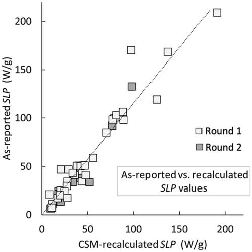
As-reported SLP values were then compared to the CSM-recalculated values, as shown in Figure 1. The data show that there is a correlation between the two, with a mean ratio of 1.15 ± 0.36, indicating a tendency for the as-reported values to be higher than the recalculated ones. Similar deviations have been previously reported from the re-analysis of literature data [15]. For the CSM analysis, the cooling curves from each of the laboratories were analyzed to identify the ‘linear loss region’ for heat transfer to the environment. This ΔT_LLR was found to be surprisingly consistent across all the laboratories, and was of order 25 K. The ‘linear loss factor’ L determined from the CSM fits was more variable, with the fitted values ranging from ca. 10–50 mW K⁻¹ for Sample 1,with a mean of 24 ± 12 mW K⁻¹; and from ca. 6 to 26 mW K⁻¹ for Sample 2, with a mean of 12 ± 6 mW K⁻¹ – values that are comparable with previous reports on similar apparatus of L values of order 5–10 mW K⁻¹ [15].

Figure 1. As-reported SLP values for Samples 1 and 2 plotted against CSM-recalculated values. The CSM analysis takes account of the inherent environmental losses in non-adiabatic calorimetry systems and is confined to the ‘linear loss region’ of the T(t) heating curves. The dotted line is a best linear fit to the data; it has a slope of ca. 1.15, indicating a tendency for the as-reported values to be higher than the recalculated ones.

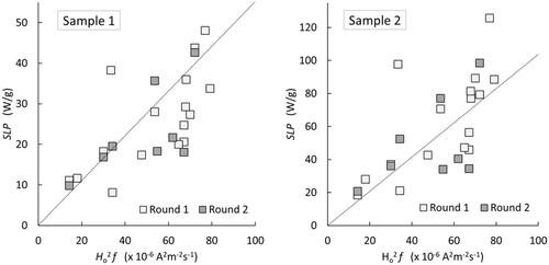
Further analysis proceeded using the CSM-recalculated fits. Figure 2 shows the measured SLP values for Samples 1 and 2, plotted as a function of H_o² f. According to Equations (1)(1) $$\mathit{SLP}=P/m_{\text{MNP}},$$(1) and (3)(3) $$P={\mu }_{0}f\oint M\left(t\right)\mathrm{ }\mathrm{d}{H}_{}\left(t\right),$$(3) it was anticipated that there should be a monotonic relationship between SLP and H_o² f. Although there is indeed a correlation between the variables – the Spearman coefficients are 0.75 and 0.80 for Samples 1 and 2 respectively – it is nonetheless clear from the data that there is significant scatter and variation in the measured data points. Furthermore, comparison in Figure 2 of the data collected in Rounds 1 and 2 of the study shows that despite significant extra control having been taken of the Round 2 measurements, there is even then no clear sign of monotonic behavior in the data. This therefore points to a possible systematic uncertainty in the measurements as undertaken in the different laboratories.

Figure 2. SLP values for Samples 1 and 2 plotted as a function of H_o² f, for which at least a monotonic trend is expected, according to Equations (1)(1) $$\mathit{SLP}=P/m_{\text{MNP}},$$(1) and (3)(3) $$P={\mu }_{0}f\oint M\left(t\right)\mathrm{ }\mathrm{d}{H}_{}\left(t\right),$$(3) . The scatter evident in the data points is an indication of interlaboratory measurement variability. Dotted lines are guides to the eye only.

3.2. Repeatability analysis

Before undertaking repeatability analysis of the data, a decision needed to be taken as to whether the ILP metric of Equation (2)(2) $$\mathit{ILP}=\mathit{SLP}/H_{\mathrm{o}}{{}^2}^{}f,$$(2) could be used for such purposes. This step was required given that the ASTM E691-18 International Standard [23] states that repeatability analysis may be undertaken only on a single measurable metric, such as the ILP, rather than on a range of measurable metrics, such as the SLP.

First, it was noted from Table 2 that both Samples 1 and 2 were polydisperse systems with PDI values well in excess of 0.1; and that the frequencies applied were all in the range from 10⁵ to 10⁶ Hz. According to this criterion [11], both would therefore be expected to lie within the LRT regime. Second, the ξ parameter of Equation (4)(4) $$\xi ={\mu }_0{M}_{\mathrm{S}}V{H}_{\mathrm{o}}/k_{\mathrm{B}}T\text{ should}\mathrm{ }\text{be} \lesssim 1,$$(4) was calculated for both samples using the measured M_S values from Table 2. For H_o = 15 kA m⁻¹ the ξ parameter was determined to be ca. 0.29 for Sample 1 and ca. 0.66 for Sample 2, both of which are less than one, and thus satisfy the criterion to lie within the LRT regime [12]. Third, the data from Table 2 was used to locate the samples on the LRT “validity map” introduced by Carrey et al. [12], which allowed for consideration of both particle size and anisotropy, alongside the external conditions (H_o and T) . According to this graphical analysis, the parameters for both samples lay well within the LRT validity region (see Supplementary Information, Figure S1). Fourth, despite the scatter, the data in Figure 2 are consistent with there being an underlying linear correlation between the SLP and H_o² f, as evidenced by Pearson coefficients of 0.91 and 0.85 for Samples 1 and 2 respectively. Fifth, a complementary version of Figure 2 was produced in which the ILP (rather than the SLP) was plotted against H_o² f (see Supplementary Information Figure S2). No correlation at all was evident between the ILP and H_o² f values, as is expected only in the LRT regime. The Pearson coefficients in this case were −0.12 and −0.26 for Samples 1 and 2 respectively. Taken together, these observations and considerations lead to the conclusion that at the fields and frequencies applied, the magnetizations of both samples responded linearly to the applied stimulus, and could therefore be characterized by the ILP parameter, as defined in Equation (2)(2) $$\mathit{ILP}=\mathit{SLP}/H_{\mathrm{o}}{{}^2}^{}f,$$(2) .

The measured SLP data was therefore converted into ILP data, which allowed for repeatability analyses to be undertaken using both the Mandel h statistic, as shown in Figure 3, and the Youden plot, as shown in Figure 4. For clarity, the Mandel h statistics in Figure 3 are shown for the Round 1 measurements only; the corresponding data for Round 2 are less comprehensive but very similar, and are given in the Supplementary Information, Figure S3. From inspection of both figures it is clear that in only one case did the h statistic exceed the ±0.5% significance level (h_crit = 2.51, for p = 17 independent measurements [23]), and that this occurred for both samples in that laboratory.

Figure 3. Mandel h statistics (relative to the mean) for Round 1 measurements, using the CSM-recalculated ILP values. Laboratory 1 is an outlier, with h values that exceed the ± 0.5% significance level, h_crit = 2.51.

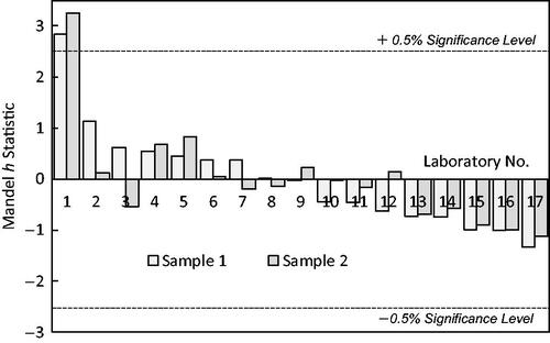
Figure 4. Youden plots of CSM-recalculated ILP values for both samples and for both rounds of measurement. The vertical and horizontal dashed lines mark the mean values for each sample, ILP_1-mean and ILP_2-mean. The diagonal line has slope ILP_2-mean/ILP_1-mean $\simeq$ 2.25.

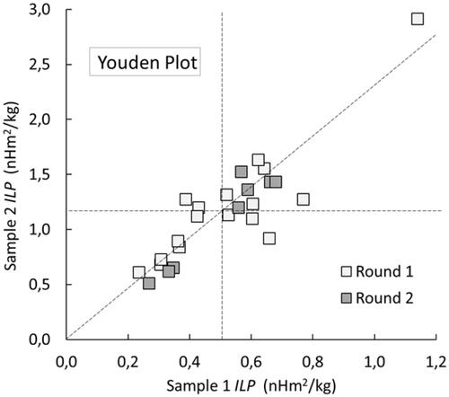
The Youden plot in Figure 4 includes the CSM-recalculated ILP data from both rounds of measurement. The outlier evident in the Mandel analysis is also seen here, as the data point in the top right-hand corner of the diagram, separated from the rest. However, also notable is the tendency for the data points to be spread out along the diagonal line with slope equal to the ratio of the mean ILP values of each sample. Such behavior is typical of Youden plots in which systematic uncertainties dominate over random errors.

Mean ILP values were then determined for each of the samples based on both the as-reported and CSM-recalculated data from Rounds 1 and 2 (see Table 1), but excluding the outlier data from Laboratory 1. On inspection of this data it is apparent that there is good agreement between the Round 1 and Round 2 data, and that the as-reported and CSM-recalculated values were not significantly different, despite the previously-mentioned tendency for the as-reported values to be overestimated, as seen in Figure 1. What is also apparent, however, is that the standard deviations on the means are large, at ca. 30% to 40% of the calculated mean. This is most likely a reflection of the systematic uncertainties seen in Figure 4, and is evidently a feature that was present in both rounds of measurement.

3.3. Correlation analysis

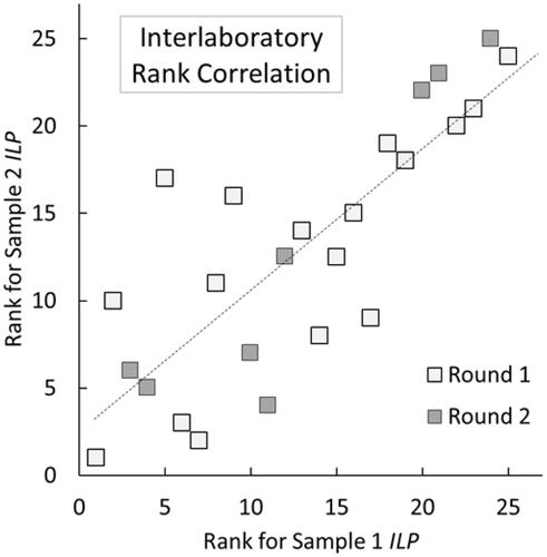
Having identified a systematic error contribution to the measured ILP values, a natural corollary was to explore whether there was a rank correlation in the data, wherein “some laboratories measured low, while others measured high”. To this end the CSM-recalculated ILP values for Samples 1 and 2, as measured in the different laboratories in both Rounds 1 and 2 (N = 25 measurements for each sample) were ranked from highest to lowest ILP, and the results plotted in Figure 5. From this plot it appears that the strongest rank correlation is between those laboratories that recorded the smallest ILP values, i.e., those that were ranked ca. 18th or above. The overall Spearman correlation coefficient was determined to be ρ = 0.81, which indicates a moderately strong correlation.

Figure 5. Interlaboratory rank correlation of the CSM-recalculated ILP values for both samples and both rounds of measurement. Each data point represents the ranking of a pair of measurements (ILP_1, ILP₂) recorded in a single laboratory in a single round. The dotted line corresponds to the best linear fit to the data; its slope is equal to the Spearman correlation coefficient for the data, ρ = 0.81.

3.4. Systematic factors analysis

In light of the large systematic variations revealed in the preceding analyses, the possible sources of such variations were considered and analyzed, as reported below.

3.4.1. Sample degradation

Liquid suspensions of MNPs, as used in this study, may be liable to aggregation, sedimentation, and to a lesser extent chemical reaction. In addition, factors such as the exposure to magnetic fields, heat or sunlight during transit may influence such effects. It was therefore impossible to guarantee a priori that the samples all arrived at each laboratory in the same state as they were when shipped from the source. Participants were therefore asked to report any visually detectable instability in the as-received samples. In practice, no such effects were noted. (In some laboratories a vortexing step was included in the measurement protocol, but this was a matter of local practice, rather than any perceived need to redisperse the samples.)

Sample aging, including environment-dependent aging [28], was another potentially confounding factor that was recognized at the outset. This was mitigated in the study protocol by asking the participants to store the samples at 5–8 °C upon receipt and to complete their measurements promptly thereafter, and by distributing fresh aliquots of centrally controlled samples in each round. In practice, all of the participants measured their samples within ca. one month of the receipt date, and there were no discernible round-to-round variations in the measured ILP values (Table 3).

Table 3. Means and standard deviations of the as-reported and CSM-recalculated ILP values for Samples 1 and 2, for both rounds of the study.

Intrinsic Loss Power, ILP [nHm^2 kg^−1]	As-reported ILP values				CSM-recalculated ILP values
	Round 1		Round 2		Round 1		Round 2
	Sample 1	Sample 2	Sample 1	Sample 2	Sample 1	Sample 2	Sample 1	Sample 2
Mean	0.52	1.13	0.49	1.07	0.49	1.09	0.50	1.09
Std. dev.	0.14	0.42	0.14	0.45	0.15	0.30	0.16	0.42

Data from the outlier, Laboratory 1, identified in Figure 3, was excluded from these calculations. Round 1 data was therefore from N = 16 laboratories; Round 2 from N = 8 laboratories.

3.4.2. Magnetic field amplitude

The study participants used a diverse range of (often bespoke) apparatus to generate the time-varying field, H (t) = H_o sin (2π f t), for their calorimetry measurements, and their as-reported values for the frequency f and magnitude H_o were used in the subsequent ILP analysis. Although frequency can be measured to high precision, standard methods do not yet exist for the in situ measurement of H_o, since standard Hall probes do not function well in the f $\approx$ 300 kHz range, and specialist probes, although they do exist [29], are not yet in widespread use. Similarly, reliable magnetic heating calibration samples have not yet been developed. As such, most laboratories relied either on extrapolations from dc field measurements, or theoretical estimates based on the known geometry of the field generation coils in their apparatus; or, in the case of those users of commercial systems, on the manufacturer’s reported H_o values. These are, however, problematic and generally unverified approaches, which may lead to unrecorded deviations between the reported H_o and the actual H_o at the sample. Furthermore, dependent on the coil geometry, field inhomogeneity over the sample volume may also be a source of unreported deviations.

To further analyze this possible source of systematic uncertainties, a post facto exercise was performed on the Round 1 data (excluding the outlier, Laboratory 1, so that N = 16). It was assumed that the only source of interlaboratory deviation in the measured ILPs was the H_o value, and correction factors were applied – by replacing H_o with H_o‘= (1 + x) H_o – to bring all the measurements in line with the overall mean. Naturally, x took both positive and negative values, hence attention was paid to its absolute value, |x|. It was found that across the 16 laboratories, the mean |x| was 14% for Sample 1, and 11% for Sample 2, with standard deviations of 8% in both cases. Perhaps more pertinently, a laboratory-specific repeatability metric y = |x₁ – x₂| was also derived, where x₁ and x₂ were the x values for Samples 1 and 2 respectively. It was found that y was less than 2% in 4/16 cases, and more than 5% in 9/16 cases. The latter figure implies that it is unlikely that unrecorded deviations in H_o were a primary source of the systematic uncertainties, as if that were the case, the laboratory-specific y metrics derived here should have been close to zero in more cases.

3.4.3. Instrument manufacturer

Although many of the study participants used bespoke field generation apparatus, it was noted that two particular commercial systems had each been used by N = 5 participants. It was found that for System 1, usable data was received from 4 partners, and that the measured mean ILPs for Samples 1 and 2 were ca. 13% and 16% higher, respectively, than the overall means. For System 2, usable data was received from 4 partners, but one of these was the outlier Laboratory 1; the measured mean ILPs for the remaining 3 laboratories, for Samples 1 and 2, were ca. 8% and 18% lower, respectively, than the overall means. Although the numbers of laboratories compared here is low, these are rather large deviations from the mean, which may indicate systematic variations between magnetic hyperthermia instrument manufacturers.

3.4.4. Thermometry

According to the measurement reports, 15 participants used a fiber-optic thermometer (from a wide range of manufacturers and models) in their apparatus; while 5 used a T-type copper/constantan thermocouple, all of which were supplied as standard with the commercial System 2 (see above). For the fiber-optic measurements, usable data was received from 13 partners: the measured mean ILP for Sample 1 was ca. 4% higher than the overall mean, while for Sample 2 it was approximately equal. For the thermocouple measurements, usable data was received from 4 partners, but one of these was the outlier Laboratory 1; the measured mean ILPs for the remaining 3 laboratories, for Samples 1 and 2, were ca. 8% and 18% lower, respectively, than the overall means.

Thermocouples can introduce at least two possible sources of uncertainty due to their electrical conductivity, viz.: (a) the occurrence of a spurious voltage jump upon field switching, which adds a sharp increase or decrease to the output temperature signal; and (b) continuous additional heating throughout the measurement window due to eddy currents within the thermocouple probes [30]. Both issues can be alleviated – the first through additional filtering, and the second by selecting thermocouples made from materials which exhibit minimal conductivity – but to our knowledge the laboratories in question had not adopted such measures.

The mechanism by which such perturbative effects might lead to suppression in the ILP values measured via thermocouple probes is not yet well understood. One possibility is that the eddy-current-generated heat within the probe might inhibit its ability to respond to changes in the temperature of its environment, and that in effect, by having heat continually flowing out of the thermocouple, it might be harder to measure heat flow coming back into the thermocouple.

In addition to the probe types used, the precise manufacturer, model and associated read-out system employed may also influence the accuracy, noise-level and response time of temperature monitoring during calorimetry [31]. Furthermore, it is known that the probe position within a sample can impact on measurement [15,32]. In light if this, probe placement advice was provided in the Round 1 measurement protocol, and precise probe positioning was mandated in Round 2. However, systematic information on the extent to which these instructions were followed was not obtained, and therefore it is not clear whether probe placement factors may have contributed to the systematic uncertainties observed.

3.4.5. Sample environment

All but one of the laboratories used non-adiabatic calorimetry equipment for the SLP measurements. For the non-adiabatic systems, two major sources of heat flow have the potential to impact upon the shape of the heating curve. First, the heat loss behavior from the sample into the surrounding environment is different for every apparatus. It is decided by factors including the sample volume, and the quality of insulation employed. The heat loss behavior may have an impact on the final result, depending on the method used to calculate the SLP: e.g., the Corrected Slope Method is designed to analyze and compensate for the losses, while the initial slope technique does not. However, even the CSM calculations may not hold in cases where the calorimeter operates under low heat generation and/or poor thermal insulation conditions. Second, over time, waste heat from the field generation coil may penetrate the sample space, producing and additional heat flow into the sample, and an artificial enhancement of the apparent heating power.

The variability of heat loss in the non-adiabatic calorimeters was tested by inspection of the CSM-recalculated data, and in particular the calculated ‘linear loss factors’ L (as described in Section 2.5). From the Round 1 data (excluding the outlier, Laboratory 1), the L parameter was found to range from 10 to 50 mW/K for Sample 1 and from 6 to 26 mW/K for Sample 2, with means of 24 and 13 mW/K respectively. These values are somewhat high compared to the 6 mW/K reported by Wildeboer et al. [15], albeit that measurement was on a sample with an ILP of ca. 2.8 nHm²kg⁻¹, and some as-yet unexplored heat loss trends as a function of the ILP may be expected. In any case, correlation analysis of the L and ILP parameters gave Pearson coefficients of 0.02 and 0.00 for Samples 1 and 2 respectively, indicating that no correlation was present.

To explore possible heat-flow effects associated with the sample volume V, correlation analysis was performed on the Round 1 data, where the choice of sample volume had been left to user preference. Excluding the data from one laboratory which had used V = 40 μL, and focusing on the remaining laboratories where V ranged from 0.5 to 2.0 ml, the analysis gave the following Pearson coefficients for Samples 1 and 2 respectively: for V versus L, ρ = 0.04 and −0.02; and for V versus ILP, ρ = −0.16 and 0.25. All four ρ values were thus close to zero. This, coupled with the observation from Table 3 that the Round 2 ILP measurements, which were all performed on a fixed 1.0 ml volume sample, were very similar to the Round 1 measurements, leads to the conclusion that V was not a significant factor in the systematic uncertainties.

Lastly, with respect to possible environmental heat flows into the sample, it was noted that although most calorimeters are designed using cooling water circulation and thermal insulation to minimize or prevent this, no data was collected in Round 1 to evaluate this. A water sample was therefore supplied in Round 2 to provide a means of measuring such background effects in the users’ equipment. Large variations in behavior were observed; Figure 6 illustrates this with temperature-time data as recorded in three different systems, including two extreme cases, and one typical case.

Figure 6. Illustration of the range of environmental heat transfer conditions under which different laboratory calorimeters operate, as measured using a centrally supplied pure water sample and the same measurement protocols as would be applied to a magnetic hyperthermia sample. The gray box highlights the period during which the magnetic field was applied. The middle curve is representative of the response recorded in most laboratories; the other two curves illustrate extreme responses.

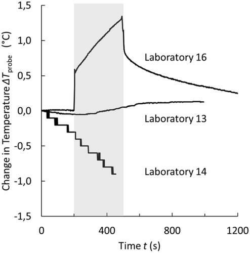
The data shown in Figure 6 from Laboratory 13 (the middle curve) was typical of most of the reported curves. This laboratory used a commercial calorimeter and a fiber-optic temperature probe. The data show that the temperature was broadly stable before the field is switched on, with a slight fall probably caused by the cooling water circulating in the coil. When the field is applied, a slight increase in the sample temperature is recorded, which begins around halfway through the field-on period. The sample temperature does not rapidly reduce after the field is switched off, indicating that the probe has a temperature similar to the surrounding environment. This behavior is most likely due to heat produced in the coil penetrating the sample space over time. However, the overall temperature rise is minimal (ΔT_max $\simeq$ 0.1 K), and as such is unlikely to impact on the resulting SLP, provided that the measured samples produce a much higher temperature rise than this background effect.

Laboratory 16 (the upper curve in Figure 6) used another commercial system, but with an as-supplied T-type thermocouple for temperature measurement. When the field was switched on, an abrupt temperature increase ΔT of ca. 0.5 K was recorded: this was most likely caused by an induced voltage in the thermocouple signal, rather than being a real change in the sample temperature [30]. Thereafter, the probe temperature increased steadily with time, most likely as the result of eddy currents flowing in the thermocouple, reaching a maximum ΔT_max $\simeq$ 1.3 K before the field was switched off. The temperature as recorded then fell abruptly by ca. 0.5 K, after which a typical cooling trend was observed, indicating that the probe was at a higher temperature than its environment. Taken together, this behavior is further evidence for extraneous perturbative effects on thermocouple measurements, as was discussed in Section 3.4.4. Solutions to these problems could be achieved by filtering electric signals and by choosing less conductive materials.

Laboratory 14 (the lower curve in Figure 6) employed a modified version of the same commercial apparatus as used in Laboratory 16, including the substitution of a fiber-optic probe for the as-supplied thermocouple, albeit the resolution of the fiber-optic was only 0.1 K, leading to ‘steps’ in the recorded temperature data. Before the field is switched on, a rather marked cooling effect was observed, presumably due to a refrigerating effect from the cooling water in the coil. This cooling trend continued throughout the measurement, with the field-on and field-off switching having no apparent effect. By the end of the measurement, a ΔT_max of ca. −0.8 K had been recorded, which would likely be sufficient to confound SLP measurement on this apparatus.

However, from the received data it was clear that Laboratories 14 and 16 were exceptions rather than the rule, and as such, samples environment effects of this kind could not explain the observed systematic variations that were observed in Figure 4, nor the rank correlations seen in Figure 5.

4. Discussion

Initial inspection of the completed measurement reports from the participating laboratories showed that there was generally a good level of experimental repeatability within any given laboratory, with run-to-run deviations of less than ±10% in 39/50 cases, and less than ±5% in 33/50 cases. In-house data analysis was also found to be generally good, with single-operator re-analysis of the raw data using the Correlated Slope Method (CSM) showing a strong linear trend (Figure 1), albeit with a tendency toward over-estimation, consistent with previous CSM-recalculation reports [15].

Given the complexity of calorimetric measurements in general, a random uncertainty of order ±5% to ±10% should most probably be considered to be acceptable (so long as the values thus obtained are duly reported with the appropriate corresponding uncertainty). However, larger intra-laboratory run-to-run deviations were noted in 11/50 cases. The three largest deviations were found to correspond to incremental changes in the measurements from run to run, which was most likely a sign of instrument drift, and as such may be regarded as experimental error. In contrast, no such trend was found for the 8/50 cases of run-to-run deviations in the range from ±10% to ±25%, implying that these were cases where significant random experimental uncertainties were present.

In addition to these random measurement uncertainties, inspection of the CSM-recalculated Specific Loss Power (SLP) data plotted as a function of H_o² f in Figure 2 showed that there was significant scatter in the data – more so than would be expected from the intra-laboratory uncertainties alone – and that the expected linear (or at least monotonic) relationship between SLP and H_o² f was not clearly present. In light of this, careful consideration was given to whether the physical and magnetic properties of the samples studied, combined with the experimental conditions used, placed the data in the Linear Response Theory (LRT) regime as described by Equation (4)(4) $$\xi ={\mu }_0{M}_{\mathrm{S}}V{H}_{\mathrm{o}}/k_{\mathrm{B}}T\text{ should}\mathrm{ }\text{be} \lesssim 1,$$(4) . It was determined that the LRT criteria were indeed met, and that as such a linear correlation was to be expected between the SLP and H_o² f parameters, as embodied in Equation (2)(2) $$\mathit{ILP}=\mathit{SLP}/H_{\mathrm{o}}{{}^2}^{}f,$$(2) as the Intrinsic Loss Power (ILP) parameter.

It may be noted that although the focus of the study was on the inter-laboratory comparisons, in retrospect it would have been useful to have conducted more extended studies in at least one laboratory. A good example here would have been to undertake a series of field-dependent SLP measurements at a single site, for which systematic uncertainties would have been minimized, allowing the anticipated linear SLP – H_o² f relationship to be observed directly. Unfortunately, this was not considered at the time, and the uncertain aging characteristics of the samples ruled out subsequent measurements.

Interlaboratory repeatability analysis was then performed using the ILP data. An initial Mandel h statistics analysis (Figure 3) showed that with the exception of one outlier (Laboratory 1), all of the measurements fell well inside the ±0.5% significance level. The outlier was also evident in Youden analysis (Figure 4), but the Youden plot also revealed that there was a clear systematic uncertainty component to the data, with the data points spread out along the ratio-of-means diagonal. The mean ILP values for both samples across both rounds of measurement were then calculated (excluding Laboratory 1) in Table 3, from which is was found that the round-to-round agreement was good, but that the measurement accuracy was poor, with standard deviations of ca. ± 30% to ± 40%.

Rank correlation analysis (Figure 5) indicated significant correlation between the ILPs measured, with a Spearman coefficient of ca. 0.81, consistent with the notion that “some laboratories measured low, while others measured high”. This then led to an analysis of possible sources of systematic uncertainties:

• Sample degradation was considered as a potential source, but discounted on the basis of the study design, and on the absence of any reported issues with suspension stability.

• Unreported deviations in the magnetic field amplitude were considered, and a post facto numerical exercise performed to establish whether deviations between the reported H_o and a postulated ‘actual’ H_o‘= (1 + x) H_o might account for the systematic uncertainties. This analysis was based on the supposition that if there was such a systematic deviation (for example one due to an over- or under-estimation by the user of the current flowing in the coil), it would affect both samples’ measurements, in a given laboratory, by an equal amount. It was found that in 9/16 cases the intra-laboratory deviations differed by more than 5% between Samples 1 and 2, indicating that it was unlikely to be the primary source of the systematic uncertainties. Although other sources of unreported deviations in H_o are possible – such as those due to field inhomogeneity, and/or variable placement of samples within the calorimeter – these were thought more likely to result in random, rather than systematic, uncertainties.

• Possible equipment-related issues were considered by examining the subset of data from those participants whose experiments were performed on one of two particular commercial systems (N = 5 of each). Interestingly, the data showed that the System 1 users reported ILP values ca. 13% and 16% higher than the overall mean, while the System 2 users reported ILP values ca. 8% and 18% lower than the overall mean, for Samples 1 and 2 respectively.

• Thermometry methods were considered, and comparisons made between users of fiber-optic thermometers and of copper/constantan thermocouples – the latter supplied as standard with the System 2 commercial systems. In this case the fiber-optic users reported ILP values within ca. 4% of the overall mean, while the thermocouple users again reported ILP values ca. 8% and 18% lower than the overall mean. Potential systematic uncertainties due to probe positioning were also considered but discounted on the basis that a uniform probe-positioning requirement was included in the Round 2 measurement protocol, with no evident impact on the systematic uncertainties.

• Sample environment factors were considered for the non-adiabatic calorimeters used by all but one participant. Analysis of the ‘linear loss factor’ L determined from the CSM-recalculations showed that although there were definite interlaboratory differences, there was no correlation between L and ILP (Pearson coefficients of ca. 0.02 and 0.00 for Samples 1 and 2). Similarly, there were no clear correlations between the sample volume used, V, and either the L or the ILP parameters. Also, uniform sample volume was included in the Round 2 measurement protocol, with no impact on the systematic uncertainties. Lastly, data acquired during Round 2 on the sample environment by having the participants measure a ‘blank’ sample of pure water showed that in most cases the heat transfer to and from the sample into its environment was small, with typical ΔT_max values of ca. 0.1 K.

Although this analysis of factors that might lead to systematic uncertainties was not exhaustive, it does represent the authors’ best efforts at understanding the correlations in Figures 4 and 5, and the large standard deviations in Table 3. None of the factors considered is an obvious candidate as the sole source of the observed systematic variation. Hence, unless there is some other factor that has escaped our attention, the source must logically be a combination of factors which, in some way that we do not yet fully understand, work together to produce the observed systematic uncertainties.

Nevertheless, it is possible as a result of this analysis to compile a list of recommended best practice for researchers in this field, as follows:

1. The magnetic field strength and its homogeneity over the sample volume should be accurately measured and the frequency verified. All properties of the magnetic field should remain stable for the complete measurement time.

2. The heat flows into and out of the sample space during normal operation should be understood and accounted for in each apparatus. The possibility of inhomogeneous heat distribution across the sample should also be considered and accounted for in an appropriate way. The measurement of ‘blank’ samples of pure water using probes placed at various positions within the sample volume is a good way to check this.

3. Thermal probes should not generate false signals or additional heat in the applied time-varying magnetic field, for which reason the use of thermocouples (unless properly shielded) is not recommended. The accuracy and response time of the chosen probe should also be verified as appropriate for the anticipated range of temperature measurements.

4. The physical and magnetic properties and stability of the material undergoing measurement should be verified in detail. Vortexing of the sample prior to measurement is recommended, to counter possible incipient aggregation effects.

5. A well-defined and repeatable measurement protocol should be employed. The protocol used in this study – comprising three consecutive heating runs plus a cooling curve measurement – is available in the Supplementary Information and is recommended. Standardization of the sample volume and placement in the calorimeter, and of the thermal probe (or probes) positioning within the sample, is also recommended.

6. Data analysis should be undertaken using, or with reference to, current best-practice methods, such as the freely available Corrected Slope Method employed in this study. If the CSM is used, attention should be paid to the linear loss factor, and this should be reported alongside the calculated SLP or ILP for a given sample.

7. Measurement reports, especially those published in the literature, should include details on the apparatus and measurement protocols used, and should always include both the applied field amplitude H_o and frequency f, alongside the chosen SLP or ILP metric. Uncertainties should be reported as the estimated random uncertainties for the laboratory in which the measurement was made, and, in instances where comparisons are made between reported measurements in different laboratories, attention should be paid to the potential impact of ca. ± 30-40% systematic uncertainties of the kind described in this study.

5. Conclusions

Of all the physical properties measured routinely in laboratories around the world, thermal properties are arguably some of the most difficult to get right. Calorimetry measurements are fraught with unexpected and undetected factors that can confound results, especially when experiments are undertaken with non-adiabatic systems. In essence, this is the problem that faces many practitioners in the emerging field of magnetic field hyperthermia today.

In the interlaboratory study reported here we have surveyed the current state-of-the-art in magnetic field hyperthermia calorimetry in Europe. We have found that although there is evidently very good repeatability within a given laboratory, the overall measurement accuracy is poor, with a significant disparity between laboratories. For the two samples that were studied, across 17 laboratories, the reported magnetic heating metrics had standard deviations on the mean of approximately ± 30% to ± 40%. These are large uncertainties. Furthermore, we have found a strong systematic component to the uncertainties, coupled with a clear rank correlation between the measuring laboratory and the reported metric. Both of these are indications of a current lack of normalization in this field.

Through analysis of the potential factors leading to these systematic uncertainties, and comparison with the data provided by the study participants, we have identified a number of possible sources of uncertainty and have considered ways in which these can be alleviated or minimized. However, no single dominant factor was identified, and significant work remains to ascertain and remove the remaining uncertainty sources. In the meantime, the results presented here clearly demonstrate the need for standardized operating procedures in the hyperthermia characterization community. In addition, the development of verified reference materials is also an increasingly pressing requirement. In this context it is interesting to note that materials other than magnetic nanoparticles may prove to be better reference materials for use in interlaboratory or calibration measurements [33].

Although we do not yet have all the answers regarding the origins of the systematic errors identified and quantified through this study, we do nonetheless have a positive outcome in the form of an agreed set of recommended best practice guidelines for magnetic hyperthermia characterization measurements. These are:

1. Verify the homogeneity and stability of the magnetic field strength and frequency applied, ideally using a suitably calibrated probe.

2. Understand and measure the heat flows into and out of the sample space, for example by recording both heating and cooling curves, and by keeping temperature excursions to moderate levels, of order ± 10–20 °C.

3. Use reliable thermal probes that do not generate false signals or additional heat, such as fiber optic probes. (Avoid thermocouples.)

4. Verify the physical/magnetic properties of the sample; and avoid aggregation. Choose a sample concentration appropriate for the intended measurement, even if this means diluting the sample so that the heat generated is manageable.

5. Define and use a repeatable measurement protocol, with standardized sample volumes and placement, and standardized probe positioning. (The Radiomag protocol is recommended, and is given in the Supplementary information.)

6. Perform at least three measurements on any given sample and estimate the random uncertainties associated with the measurement. (Repeatability levels should typically be within ±10%, and preferably within ±5%; larger values may indicate instrumental or procedural issues that should be resolved.)

7. Review and use current best-practice methods for data analysis. (The CSM “calibrated slope method” is recommended, and is freely available [25]).

8. Always report experimental details, H_o and f, alongside the chosen SLP or ILP metric; and report estimates of the local random uncertainties derived from the repeat measurements.

In conclusion, we believe that our study provides a first step in the prenormative validation of magnetic field hyperthermia research methods, and will be an aid to future standardization development, and the continued transition of this exciting new technology from the laboratory to the clinic.

Acknowledgements

The RADIOMAG consortium members participating in this study and not referenced in the authorship are explicitly named here. (See the Supplementary Information for a complete listing, with affiliations.) Nanoparticle synthesis was undertaken by: Dermot Brougham, Daniel Horak, Sophie Laurent, Claudio Sangregorio, Nguyễn Thanh, and Ladislau Vekas. Measurements were undertaken by: Manuel Bañobre, Marko Bošković, Dermot Brougham, Julian Carrey, Nico Cassinelli, Marco Cobianchi, Luc Dupré, Eleni Efthimiadou, Liliana Ferreira, José Angel Garcia, Andrea Guerrini, Claudia Innocenti, Carlton Jones, Georgios Kasparis, Alessandro Lascialfari, Fang-Yu Lin, Patricia Monks, Teresa Pellegrino, Fernando Plazaola, Claudio Sangregorio, Beatriz Sanz Sagué, Niccolò Silvestri, Mahendran Subramanian, Francisco Terán, Nguyễn Thanh, Etelka Tombácz, Le Duc Tung, and Vlasta Zavisova.

Disclosure statement

No potential conflict of interest was reported by the author(s).

Supplementary material

See the Supplementary Material for details of the recommended measurement protocol used in Round 2; and for full sets of the CSM-recalculated data as used in the study.

Data availability statement

The data that support the findings of this study are publicly available for download. The files are uploaded in the Zenodo repository under the title “Radiomag Interlaboratory Comparison of Magnetic Hyperthermia Characterisation Measurements: Data” DOI: https://zenodo.org/record/4281154#.YEiMBk6g82w.

Additional information

Funding

This article is based upon work supported by the COST action [RADIOMAG TD1402], supported by COST (European Cooperation in Science and Technology). The financial support of the DFG research grants “quantMPI: Establishment of quantitative Magnetic Particle Imaging (MPI) application oriented phantoms for preclinical investigations “(TR 408/9-1) and ‘Matrix in Vision”. [SFB 1340/1 2018, no 372486779, projects A02 and B02] are also gratefully acknowledged. Additional financial support was received from the Spanish Ministry of Economy and Competitiveness through the grants RED2018-102626-T, MAT2017-85617-R, MAT2017-86826-R and the “Severo Ochoa” Program for Centers of Excellence in R&D [SEV-2016-0686]. Additional financial support was received from the Portuguese Foundation for Science and Technology (FCT) under UID/MULTI/04046/2019 (BioISI).

References

- “International Agency for Research on Cancer, GLOBOCAN 2018 accessed via Global Cancer Observatory,” 2018.
- Kantoff PW, Schuetz TJ, Blumenstein BA, et al. Overall survival analysis of a phase II randomized controlled trial of a Poxviral-based PSA-targeted immunotherapy in metastatic castration-resistant prostate cancer. J Clin Oncol. 2010;28(7):1099–1105. Hoos A, Britten CM, Huber C, et al. A methodological framework to enhance the clinical success of cancer immunotherapy. Nat Biotechnol. 2011;29(10):867–870.
- Miyamoto H, Messing EM, Chang C. Androgen deprivation therapy for prostate cancer: current status and future prospects. Prostate. 2004;61(4):332–353. Hellerstedt BA, Pienta KJ. The current state of hormonal therapy for prostate cancer. CA Cancer J Clin. 2009;52:154.
- Thiesen B, Jordan A. Clinical applications of magnetic nanoparticles for hyperthermia. Int J Hyperthermia. 2008;24(6):467–474.
- Bañobre-López M, Teijeiro A, Rivas J. Magnetic nanoparticle-based hyperthermia for cancer treatment. Rep Pract Oncol Radiother. 2013;18(6):397–400.
- Dutz S, Hergt R. Magnetic particle hyperthermia-a promising tumour therapy? Nanotechnology. 2014;25(45):452001.
- Johannsen M, Gneveckow U, Eckelt L, et al. Clinical hyperthermia of prostate cancer using magnetic nanoparticles: presentation of a new interstitial technique. Int J Hyperthermia. 2005;21(7):637–647; Wust P, Gneveckow U, Johannsen M, et al. Magnetic nanoparticles for interstitial thermotherapy–feasibility, tolerance and achieved temperatures. Int J Hyperthermia. 2006;22(8):673–685; Johannsen M, Gneveckow U, Thiesen B, et al. Thermotherapy of prostate cancer using magnetic nanoparticles: Feasibility, imaging, and three-dimensional temperature distribution. Eur Urol. 2007;52(6):1653–1661; Maier-Hauff K, Rothe R, Scholz R, et al. Intracranial thermotherapy using magnetic nanoparticles combined with external beam radiotherapy: Results of a feasibility study on patients with glioblastoma multiforme. J Neurooncol. 2007;81(1):53–60; Maier-Hauff K, Ulrich F, Nestler D, et al. Efficacy and safety of intratumoral thermotherapy using magnetic iron-oxide nanoparticles combined with external beam radiotherapy on patients with recurrent glioblastoma multiforme. J Neurooncol. 2011;103(2):317–324.
- Dutz S, Kettering M, Hilger I, et al. Magnetic multicore nanoparticles for hyperthermia-influence of particle immobilization in tumour tissue on magnetic properties. Nanotechnology. 2011;22(26):265102; Perigo EA, Hemery G, Sandre O, et al. Fundamentals and advances in magnetic hyperthermia. Appl Phys Rev. 2015;2(4):041302; Blanco-Andujar C, Teran FJ, Ortega D. Chapter 8 - current outlook and perspectives on nanoparticle-mediated magnetic hyperthermia. In: Mahmoudi M, Laurent S, editors. Iron Oxide Nanoparticles for Biomedical Applications. Amsterdam: Elsevier; 2018. p. 197–245; Chang D, Lim M, Goos JACM, et al. Biologically targeted magnetic hyperthermia: Potential and limitations. Front Pharmacol. 2018;9:831.
- Note: The SLP parameter is also sometimes referred to in the literature as the ‘specific absorption rate’, SAR. This should not be confused with the clinical use of the SAR terminology, which refers exclusively to power dissipation in tissue.
- Kallumadil M, Tada M, Nakagawa T, et al. Suitability of commercial colloids for magnetic hyperthermia. J Magn Magn Mater. 2009;321(10):1509–1513.
- Rosensweig RE. Heating magnetic fluid with alternating magnetic field. J Magn Magn Mater. 2002;252:370–374.
- Carrey J, Mehdaoui B, Respaud M. Simple models for dynamic hysteresis loop calculations of magnetic single-domain nanoparticles: application to magnetic hyperthermia optimization. J Appl Phys. 2011;109(8):083921.
- Dutz S, Clement JH, Eberbeck D, et al. Ferrofluids of magnetic multicore nanoparticles for biomedical applications. J Magn Magn Mater. 2009;321(10):1501; Lee JH, Jang JT, Choi JS, et al. Exchange-coupled magnetic nanoparticles for efficient heat induction. Nat Nanotechnol. 2011;6:418; Hugounenq P, Levy M, Alloyeau D, et al. Iron oxide monocrystalline nanoflowers for highly efficient magnetic hyperthermia. Journal of Physical Chemistry C 2012;116(29):15702–12; Behdadfar B, Kermanpur A, Sadeghi-Aliabadi H, et al. Synthesis of high intrinsic loss power aqueous ferrofluids of iron oxide nanoparticles by citric acid-assisted hydrothermal-reduction route. J Solid State Chem. 2012;187:20–2; Guardia P, Di Corato R, Lartigue L, et al. Water-soluble iron oxide nanocubes with high values of specific absorption rate for cancer cell hyperthermia treatment. ACS Nano. 2012;6(4):3080; Martinez-Boubeta C, Simeonidis K, Makridis A, et al. Learning from nature to improve the heat generation of iron-oxide nanoparticles for magnetic hyperthermia applications. Scientific Reports. 2013;3:1652; Blanco-Andujar C, Ortega D, Southern P, et al. High performance multi-core iron oxide nanoparticles for magnetic hyperthermia: microwave synthesis, and the role of core-to-core interactions. Nanoscale. 2015;7(5):1768–75; Shubitidze F, Kekalo K, Stigliano R, et al. Magnetic nanoparticles with high specific absorption rate of electromagnetic energy at low field strength for hyperthermia therapy. J Appl Phys. 2015;117(9):094302.
- Wells J, Kazakova O, Posth O, et al. Standardisation of magnetic nanoparticles in liquid suspension. J Phys D Appl Phys. 2017;50(38):383003.
- Wildeboer RR, Southern P, Pankhurst QA. On the reliable measurement of specific absorption rates and intrinsic loss parameters in magnetic hyperthermia materials. J Phys D Appl Phys. 2014;47(49):495003.
- Makridis A, Curto S, van Rhoon GC, et al. A standardisation protocol for accurate evaluation of specific loss power in magnetic hyperthermia. J Phys D Appl Phys. 2019;52(25):255001.
- OECD (Organisation for Economic Co-operation and Development). Guidance document on the validation and international acceptance of new of updated test methods for hazard assessment. 2005.
- Spirou S, Basini M, Lascialfari A, et al. Magnetic hyperthermia and radiation therapy: radiobiological principles and current practice †. Nanomaterials (Basel). 2018;8(6):401.
- COST Action “RADIOMAG”. website: http://www.cost-radiomag.eu/
- Roebben G, Rasmussen K, Kestens V, et al. Reference materials and representative test materials: the nanotechnology case. J Nanopart Res. 2013;15:1455.
- Rad AM, Janic B, Iskander ASM, et al. Measurement of quantity of iron in magnetically labeled cells: comparison among different UV/VIS spectrometric methods. BioTechniques. 2007;43(5):627–628, 630, 632 passim.,
- Frot D, Jacob D. US patent 2012/0250019 (priority date 2009/6/26).
- ASTM International. ASTM E691-18 standard practice for conducting an interlaboratory study to determine the precision of a test method. West Conshohocken (PA): ASTM International; 2018.
- Dunlop DJ, Özdemir Ö. Rock magnetism: fundamentals and frontiers. Cambridge: Cambridge University Press; 1997.
- Note: Matlab and Excel versions of the CSM analysis programs are freely available at www.resonantcircuits.com.
- Youden WJ. Graphical diagnosis of interlaboratory test results. J Qual Technol. 1972;4(1):29. Croarkin C, Guthrie W. NIST/SEMATECH e-handbook of statistical methods. 2003. DOI:https://doi.org/10.18434/M32189.
- Mandel J. The validation of measurement through interlaboratory studies. Chemom Intell Lab Syst. 1991;11(2):109–119.
- Bogart LK, Blanco-Andujar C, Pankhurst QA. Environmental oxidative aging of iron oxide nanoparticles. Appl Phys Lett. 2018;113(13):133701.
- Note: For example, the “AC Magnetic Field Probe” manufactured by Nanoscience Laboratories Limited, Newcastle under Lyme, UK.
- Shir F, Mavriplis C, Bennett LH. Instrum Sci. Technol. 2005;33(6):661–671.
- Natividad E, Castro M, Mediano A. Adiabatic vs. non-adiabatic determination of specific absorption rate of ferrofluids. J Magn Magn Mater. 2009;321(10):1497–1500.
- Wang SY, Huang S, Borca-Tasciuc DA. Potential sources of errors in measuring and evaluating the specific loss power of magnetic nanoparticles in an alternating magnetic field. IEEE Trans Magn. 2013;49(1):255.
- Natividad E, Castro M, Mediano A. Accurate measurement of the specific absorption rate using a suitable adiabatic magnetothermal setup. Appl Phys Lett. 2008;92(9):093116.