Multiple imputation of longitudinal categorical data through bayesian mixture latent Markov models

ABSTRACT

Standard latent class modeling has recently been shown to provide a flexible tool for the multiple imputation (MI) of missing categorical covariates in cross-sectional studies. This article introduces an analogous tool for longitudinal studies: MI using Bayesian mixture Latent Markov (BMLM) models. Besides retaining the benefits of latent class models, i.e. respecting the (categorical) measurement scale of the variables and preserving possibly complex relationships between variables within a measurement occasion, the Markov dependence structure of the proposed BMLM model allows capturing lagged dependencies between adjacent time points, while the time-constant mixture structure allows capturing dependencies across all time points, as well as retrieving associations between time-varying and time-constant variables. The performance of the BMLM model for MI is evaluated by means of a simulation study and an empirical experiment, in which it is compared with complete case analysis and MICE. Results show good performance of the proposed method in retrieving the parameters of the analysis model. In contrast, competing methods could provide correct estimates only for some aspects of the data.

KEYWORDS:

• Bayesian mixture latent Markov models
• missing data
• longitudinal analysis
• multiple imputation

1. Introduction

Sociological, psychological and medical research studies are often performed by means of longitudinal designs, and with variables measured on a categorical scale. An example is the LISS (Longitudinal Internet Studies for the Social Sciences) panel study consisting of periodically administered Internet surveys by CentERData (Tilburg University, The Netherlands) to a representative sample of the Dutch population, and covering a broad range of topics such as health, religion, work, and the like.

Different from cross-sectional studies, missing data in longitudinal studies may not only concern partial missingness within a single measurement occasion but may also take the form of complete missing information for certain occasions as a result of missing visits (or complete missingness) or subjects dropping out from the study.¹ When data are missing at random (MAR)² and the missingness occurs in the covariates of the analysis model, it is well known that ignoring the missing data (i.e. retaining only the complete cases in the dataset) can lead to biased and inaccurate inferences. While computationally cheap, this method can lead analysts to wrong conclusions under the MAR assumption. Multiple Imputation (MI) is a method developed by [16] which allows separating the missing data handling from the substantive analyses of interest, and moreover takes the additional uncertainty resulting from the missing values into account. Under the MAR assumption, in MI the missing values of a dataset are replaced with M>1 sets of values sampled from the distribution of the missing data given the observed data, $Pr\left({\mathbf{y}}^{mis}|{\mathbf{y}}^{obs}\right)$. In order to be able to do this, an imputation model is needed. The substantive model of interest is then estimated on each of the M completed datasets, where the M sets of estimates can be pooled through the rules provided by [7,16]. Throughout this paper, we assume the missing data are MAR, and we will deal with methods for incomplete covariates of the analysis model.³

When imputing missing longitudinal data, the imputation model must fulfill several requirements in order to produce valid imputations. In particular, an imputation model for longitudinal analysis should:

1. capture dependencies among variables within measurement occasions;

2. capture overall dependencies between time points resulting from the fact that individuals differ from one another in a systematic way;

3. capture potential stronger relationships between adjacent time points;

4. automatically (i.e. without explicit specification) capture complex relationships in the data, such as higher-order interactions and non-linear associations;

5. respect the measurement scale of the variables (continuous/categorical).

In particular, requirement 4 is motivated by the fact that the imputed datasets could be re-used for several types of analyses, in which different aspects of the data need to be taken into account. An imputation model that can automatically describe all the relevant associations of the data provides datasets that can be re-used in different contexts. Conversely, if an imputation model requires explicit specification of interaction terms and other complex relationships, the imputed datasets are likely to be tailored only for some specific analyses, and the imputation step should be re-performed according to the particular problem under investigation. Furthermore, specifying all the complex interactions that might arise in a dataset can be a difficult and tedious task [23].

One possible approach for the MI of longitudinal categorical data is given by the implementation of the MICE technique [19,20] (a full conditional specification method) with generalized linear models using a logistic link function after converting the data from long to wide format. That is, converting the dataset in such a way that the different time points (the single rows of the dataset in the long format) become columns in the wide format.⁴ In such a way, relationships among the variables at different time points can correctly be captured by MICE and reproduced in the imputations [1,26]. This occurs because MICE works by estimating a series of logistic regression models, in which the variables with missing values are treated as outcomes. Each of these outcomes is sequentially regressed on all the other variables present in the dataset; imputation values are then drawn from the resulting models. Despite the advantages and the ease of implementation of the method, MICE is not always guaranteed to work. In the first place, notwithstanding its good performances in simulation studies, convergence to the true distribution of the missing data is not ensured, since the method lacks of theoretical and statistical foundation [23]. Second, conversion from long to wide format causes the number of variables to be imputed (and to be used as predictors) to grow linearly with the number of time points T, slowing down computations and requiring regularization techniques if the sample size is small. Lastly, by default MICE only includes linear main effects into the imputation model. While the routine allows for the specification of more complex relationships when these are needed in the analysis model, it is not always clear at the imputation stage what relationships are needed for future analyses, and thus requirement 4 above might not be always met.

An alternative solution for categorical data is represented by mixture or latent class (LC) models [12], proposed and shown to provide good results as imputation models by [3,23]. Mixture modeling allows for flexible joint-density estimation of the categorical variables in the dataset and requires only the specification of the number of LCs K. When K is set large enough, the model can automatically capture the relevant associations of the joint distribution of the variables [14,23], achieving requirement 4. However, standard LC models are better suited for cross-sectional datasets because they do not account for the longitudinal architecture of the data, and, accordingly, do not satisfy requirement 3 above.

A natural extension of the LC model to longitudinal categorical data, which in addition accounts for unobserved heterogeneity between units, is represented by the mixture Latent Markov (MLM) model [11,21,22]. This model, also known in the literature as mixed Hidden Markov model or random-effects Hidden Markov model, is described more in detail by [13] and [5]. With the MLM model, subjects are clustered at two levels. At the higher level, a time-constant LC variable groups the units with similar time-varying patterns with each other, meeting in this way requirement 2. At the within-subject level, dynamic latent states (LSs; i.e. LCs that can vary over time) are specified for each time point, and -with the first-order Markov assumption- the LS distribution at a specific time point depends only on the LS occupied at the previous time occasion. From an MI point of view, the dynamic LSs help accounting for stronger dependencies across adjacent time points, satisfying requirement 3 above. Furthermore, the distribution of the observed variables at a specific time point depends not only on the time-constant LCs but also on the dynamic LSs, allowing to take dependencies within time points into account, thus meeting requirements 1 and 4. Lastly, the model respects the data scale (requirement 5) by assuming Multinomial distributions for all variables in the measurement model. As a further advantage, the MLM model can produce imputations also for time-constant variables with missing values, when present in the dataset at hand. Note that this imputation model differs from the one proposed in [24], where a Multilevel Latent Class (MLC) model is used to impute multilevel categorical data. In fact, while the time-constant latent classes in the MLM model serve the same purpose as the higher-level classes of the MLC model, the two methods differ for the specification of the lower-level models. On the one hand, the MLC model assumes static latent classes for the lower-level units, which makes it suitable for the imputation and classification of data coming from different populations observed at a specific point in time. On the other hand, the MLM model assumes dynamic latent states for the within-subject observations, which makes this model more fit with data collected across different time points, as auto-correlations are explicitly taken into account by the latent Markov structure of the model. If we were to impute longitudinal data with the MLC model, potential auto-correlations required by the analysis model might be lost or become weaker due to the imputation step, leading in this way to invalid inferences and incorrect conclusions.

While the literature has mainly focused on obtaining unbiased estimates of MLM models in the presence of missing data (e.g. [4] use an event-history extension of the model for situations of informative drop-out), in this article, we investigate the performance of MLM models as an MI tool for missing categorical longitudinal data. The model is implemented under a Bayesian paradigm. The choice of Bayesian modeling in MI is mainly motivated by two arguments: (a) it naturally yields the posterior distribution of the missing data given the observed data; and (b) it automatically takes into account the variability of the imputation model parameter, yielding proper imputations [17].

The outline of the paper is as follows. In Section 2, the model is formally introduced, and the model selection issue is addressed. Sections 3 and 4 describe a simulation and an empirical study evaluating the performance of the Bayesian MLM (BMLM) imputation model. The authors provide final remarks in Section 5.

2. The Bayesian mixture latent Markov model for multiple imputation

Bayesian estimation of the MLM model requires defining the exact data generating model, such as the number of classes for the mixture part and the number of states for the latent Markov chain, as well as the prior distribution of the model parameters. This allows obtaining $Pr\left(\mathit{\theta }|{\mathbf{y}}^{obs}\right)$, the posterior distribution of the unknown model parameters given the observed data ${\mathbf{y}}^{obs}$. In MI, the M sets of imputations are obtained from the posterior predictive distribution of the missing data, i.e. $Pr\left({\mathbf{y}}^{mis}|{\mathbf{y}}^{obs}\right)=\int Pr\left({\mathbf{y}}^{mis}|\mathit{\theta }\right)Pr\left(\mathit{\theta }|{\mathbf{y}}^{obs}\right)d\mathit{\theta }$. To achieve this, M parameter values ${\mathit{\theta }}^{\left(m\right)}(m=1,\dots ,M)$ are first sampled from $Pr\left(\mathit{\theta }|{\mathbf{y}}^{obs}\right)$, and subsequently the imputations are drawn from $Pr\left({\mathbf{y}}^{mis}|{\mathit{\theta }}^{\left(m\right)}\right)$.

2.1. Data generating model and prior distribution

We will assume fixed measurement occasions t ($t=1,\dots ,T$) over all subjects and variables. For the ith unit ($i=1,\dots ,n$), $y_{itj}$ indicates the value observed for the jth time-varying categorical variable ($j=1,\dots ,J$) at time t, with $y_{itj}\in \{1,\dots ,r,\dots ,R_j\}$ (therefore $R_j$ represents the number of categories for the jth variable). The J-dimensional vector of observed values for unit i at time t is denoted by ${\mathbf{y}}_{it}={\mathbf{r}}_t$, where $\mathbf{r}$ represents a generic pattern, and ${\mathbf{y}}_i=\tilde{\mathbf{r}}$ is the vector of responses at all time points for unit i.

Often, also time-constant variables (such as the subject's gender) are present in the dataset. When this is the case, $z_{ip}$ is used to denote the value on the pth ($p=1,\dots ,P$) time-constant variable observed for unit i. Here $z_{ip}\in \{1,\dots ,u,\dots ,U_p\}$ and the P-dimensional time-constant pattern observed for i is given by ${\mathbf{z}}_i=\mathbf{u}$.

The MLM describes the joint distribution of the data $Pr({\mathbf{z}}_i,{\mathbf{y}}_i)$ by introducing two types of categorical latent variables: a time-constant LC variable w ($w\in \{1,\dots ,l,\dots ,L\}$) and a sequence of dynamic LSs $s_1,s_2,\dots ,s_t,\dots ,s_T|w=l$ $(s_t\in \{1,\dots ,k,\dots ,K\}\mathrm{\forall }t$). For the first-order Markov assumption, the distribution of the LSs at time t is dependent on the past only through state at time t−1, that is $Pr(s_t|s_{t-1},\dots ,s_1,w=l)=Pr(s_t|s_{t-1},w=l)$. Furthermore, the model assumes local independence for the distribution of both time-constant and time-varying variables conditioned on the latent variables: $Pr({\mathbf{y}}_{it}={\mathbf{r}}_t|s_t=k,w=l)=\prod _{j}Pr(y_{itj}=r|s_t=k,w=l)$ and $Pr({\mathbf{z}}_i=\mathbf{u}|w=l)=\prod _{p}Pr(z_{ip}=u|w=l)$.

The MLM model is composed of four parts:

• the latent class probabilities for the time-constant latent clusters, expressed by $Pr(w=l)={\omega }_l\mathrm{\forall }l$;

• the latent states probabilities, which represent the distribution of the LSs at each time point; these are given by:

  1. the initial state probabilities, which describe the distribution of the latent states at time t=1, and denoted by $Pr(s_1=\kappa |w=l)={\nu }_{\kappa l}\mathrm{\forall }\kappa ,l$;

  2. the transition probabilities, the probabilities for a unit to switch from state $s_{t-1}|w=l$ to state $s_t|w=l$ ($t=2,\dots ,T$), and indicated with $Pr(s_t=k|s_{t-1}=q,w=l)={\xi }_{q,k\left(t\right)l}$;

• the conditional response probabilities of the time-constant variables given the LC w, denoted with $Pr(z_{ip}=u|w=l)={\lambda }_{upl}$ for the pth variable and $Pr({\mathbf{z}}_i=\mathbf{u}|w=l)={\mathrm{\Lambda }}_{\mathbf{u}l}$ for the whole pattern: under local independence, ${\mathrm{\Lambda }}_{\mathbf{u}l}=\prod _p{\lambda }_{upl}$;

• the emission probabilities, which define the probability of the time-varying variables conditioned on the LC w and the LS at time t: $Pr(y_{itj}=r|s_t=k,w=l)={\phi }_{rtjkl}$, and – for the local independence – $Pr({\mathbf{y}}_{it}={\mathbf{r}}_t|s_t=k,w=l)={\mathrm{\Phi }}_{\mathbf{r}tkl}=\prod _j{\phi }_{rtjk}$.

Given the model components above, the MLM model describes the probability of the observed variables as (1) $Pr({\mathbf{z}}_i=\mathbf{u},{\mathbf{y}}_i=\tilde{\mathbf{r}})=\sum _l{\omega }_l{\mathrm{\Lambda }}_{\mathbf{u}l}{\pi }_{\tilde{\mathbf{r}}l},$(1) where, at the within-subject level, (2) ${\pi }_{\tilde{\mathbf{r}}l}=Pr(y_i=\tilde{\mathbf{r}}|w=l)=\sum _{s_1,\dots ,s_T}{\nu }_{\kappa l}{\mathrm{\Phi }}_{\mathbf{r}1kl}\prod _{t>1}{\xi }_{q,k\left(t\right)l}{\mathrm{\Phi }}_{\mathbf{r}tkl}.$(2)

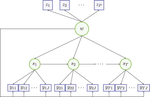
Figure 1 represents the path diagram of the data generating model. The picture stresses the double task executed by the subject-level mixture component w: capturing dependencies among the time-constant variables and overall dependencies between all time points. Figure 1 also shows how the LS $s_t$ at time t affects the distribution of both $s_{t+1}$ and ${\mathbf{y}}_{it}$, capturing dependencies between variables within time point t (by means of the emission probabilities) as well as relationships between adjacent time points (by means of the transition probabilities). With such a model configuration, requirement 2 of Section 1 is satisfied with the time-constant latent variable w, while requirements 1 and 3 are met by means of the latent Markov structure assumed upon the time-varying variables. Importantly, the model can also be implemented in the absence of the time-constant variables, which involves dropping the term ${\mathrm{\Lambda }}_{\mathbf{u}l}$ from equation (1) and the nodes representing the time-constant variables $z_{i1},\dots ,z_{iP}$ from Figure 1.

Figure 1. Graphical representation of MLM model. w: time-constant latent class variable; z: time-constant variables; s: dynamic latent variable; y: time-varying variables.

The transition probabilities ${\xi }_{q,k\left(t\right)l}$ are stored in T $K\times K$ squared matrices ${\mathit{X}}_l^t\mathrm{\forall }t\ge 2$. ${\mathit{X}}_l^t$ is a stochastic matrix, the rows of which must sum to 1: an entry in row q and column k of the matrix represents the probability for a unit to switch from state q at time t−1 to state k at time t. The qth row of ${\mathit{X}}_l^t$ will be denoted by ${\mathit{\xi }}_{ql}^t$.

In order to improve class identification, and to reduce the computational burden during the estimation step, we will assume homogeneous transition and emission probabilities across time points: ${\xi }_{q,k\left(t\right)l}={\xi }_{q,k\left(h\right)l}\mathrm{\forall }t\ne h$ and $t,h\ge 2$ and ${\phi }_{rtjkl}={\phi }_{rhjkl}$, which entails ${\mathrm{\Phi }}_{\mathbf{r}tk}={\mathrm{\Phi }}_{\mathbf{r}hk}\mathrm{\forall }t\ne h$ and $t,h\ge 1$. Thus, the time-identifier subscript will be dropped from the transition and emission probabilities in the remainder of this article, i.e. ${\xi }_{q,k\left(t\right)l}={\xi }_{q,kl},{\mathit{X}}_l^t={\mathit{X}}_l$ and ${\mathit{\xi }}_{ql}^t={\mathit{\xi }}_{ql}\mathrm{\forall }t\ge 2$, and ${\phi }_{rtjk}={\phi }_{rjk},{\mathrm{\Phi }}_{\mathbf{r}tk}={\mathrm{\Phi }}_{\mathbf{r}k}\mathrm{\forall }t\ge 1$.

For the Bayesian specification of the model, distributional assumptions must be made for all variables and parameters in model (1)–(2). Since all (latent and observed) variables in the model are categorical, a Multinomial distribution will be adopted for each of them. Formally:

• $w\sim Multinomial\left(\mathit{\omega }\right)$, with $\mathit{\omega }$ the latent weights vector $({\omega }_1,\dots ,{\omega }_L)$;

• $z_{ip}|w=l\sim Multinomial\left({\mathit{\lambda }}_{pl}\right)$, with ${\mathit{\lambda }}_{pl}=({\lambda }_{1pl},\dots ,{\lambda }_{U_{p}pl})\mathrm{\forall }p,l$;

• $s_1|w=l\sim Multinomial\left({\mathit{\nu }}_l\right)$, where ${\mathit{\nu }}_l$ is the initial state probabilities vector $({\nu }_{1l},\dots ,{\nu }_{Kl})\mathrm{\forall }l$;

• $s_t|s_{t-1}=q,w=l\sim Multinomial\left({\mathit{\xi }}_{ql}\right)\mathrm{\forall }t>1,l$;

• $y_{itj}|s_t=k,w=l\sim Multinomial\left({\mathit{\phi }}_{jkl}\right)$, with ${\mathit{\phi }}_{jkl}$ the probability vector $({\phi }_{1jkl},\cdots ,{\phi }_{rjkl},\cdots ,{\phi }_{R_{j}jkl})\mathrm{\forall }j,k,l$.

We denote by $\mathit{\theta }$ the whole parameter vector, i.e. $\mathit{\theta }=(\mathit{\omega },{\mathit{\lambda }}_{11},\cdots ,{\mathit{\lambda }}_{PL},{\mathit{\nu }}_1,\dots ,{\mathit{\nu }}_L,{\mathit{X}}_1,\dots ,{\mathit{X}}_L,{\mathit{\phi }}_{111},\dots ,{\mathit{\phi }}_{JKL})$. The conjugate of the Multinomial is the Dirichlet distribution. Hence we will set:

• $\mathit{\omega }\sim Dirichlet\left(\mathit{\eta }\right)$, with $\eta =({\eta }_1,\dots ,{\eta }_L),{\eta }_l>0\mathrm{\forall }l$;

• ${\mathit{\lambda }}_{pl}\sim Dirichlet\left({\mathit{\zeta }}_{pl}\right)$, with ${\mathit{\zeta }}_{pl}=({\zeta }_{1pl},\dots ,{\zeta }_{U_{p}pl})$ and ${\zeta }_{upl}>0\mathrm{\forall }u,p,l$.

• ${\mathit{\nu }}_l\sim Dirichlet\left(\mathit{\alpha }\right)$, with $\mathit{\alpha }=({\alpha }_1,\dots ,{\alpha }_K),{\alpha }_{\kappa }>0\mathrm{\forall }\kappa ,l$;

• ${\mathit{\xi }}_{ql}\sim Dirichlet\left(\mathit{\gamma }\right)$, with $\mathit{\gamma }=({\gamma }_1,\dots ,{\gamma }_K),{\gamma }_k>0\mathrm{\forall }k,l$;

• ${\mathit{\phi }}_{jkl}\sim Dirichlet\left({\mathit{\delta }}_{jk}\right)$, with ${\mathit{\delta }}_{jk}=({\delta }_{1jk},\dots ,{\delta }_{R_{j}jk}),{\delta }_{rjk}>0\mathrm{\forall }r,j,k,l$ .

$\mathit{\eta },{\mathit{\zeta }}_{pl},\mathit{\alpha },\mathit{\gamma }$ and ${\mathit{\delta }}_{jk}$ are called hyperparameters of the model. The resulting posterior distributions are :

• $\mathit{\omega }|w=l,\mathit{\eta }\sim$$Dirichlet({\eta }_1+\sum _{i=1}^n{\mathcal{I}}_i(w=1),\dots ,{\eta }_L+\sum _{i=1}^n{\mathcal{I}}_i(w=L\left)\right)$, where ${\mathcal{I}}_i(w=l)=1$ if w=l for unit i and 0 otherwise;

• ${\mathit{\lambda }}_{pl}|w=l,{\mathbf{z}}^{obs},{\mathit{\zeta }}_{pl}\sim$$Dirichlet({\zeta }_{1pl}+\sum _{i:w=l}\mathcal{I}(z_{ip}=1),\dots ,{\zeta }_{U_{p}pl}+\sum _{i:w=l}\mathcal{I}(z_{ip}=U_p\left)\right)$, where where $\mathcal{I}(z_{ip}=u)=1$ if $z_{ip}=u$ and $z_{ip}\in {\mathbf{z}}^{obs}$ and 0 otherwise;

• $\mathit{\nu }|s_1,w=l,\mathit{\alpha }\sim Dirichlet({\alpha }_1+\sum _{i:w=l}{\mathcal{I}}_{i1}(s_1=1),\dots ,{\alpha }_K+\sum _{i:w=l}{\mathcal{I}}_{i1}(s_1=K,w=l\left)\right)$;

• ${\mathit{\xi }}_q|s_{t-1},s_t,w=l,\mathit{\gamma }\sim Dirichlet({\gamma }_1+\sum _{i,t:w=l,s_{t-1}=q}{\mathcal{I}}_{it}(s_t=1),\dots ,{\gamma }_K+\sum _{i,t:w=l,s_{t-1}=q}{\mathcal{I}}_{it}(s_t=K\left)\right)$;

• ${\mathit{\phi }}_{jk}|s_t,w=l,{\mathbf{y}}^{obs},{\mathit{\delta }}_{jk}\sim \text{Dirichlet}({\delta }_{1jk}+\sum _{i,t:w=l,s_t=k}\mathcal{I}(y_{itj}=1),\dots ,{\delta }_{R_{j}jk}+\sum _{i,t:w=l,s_t=k}\mathcal{I}(y_{itj}=R_j\left)\right)$, where $\mathcal{I}(y_{itj}=r)=1$ if $y_{itj}=r$ and $y_{itj}\in {\mathbf{y}}^{obs}$ and 0 otherwise.

With symmetric Dirichlet priors (i.e. all the hyerparameters are set to the same value for each of the specified Dirichlet), increasing the value of the hyperparameters has the effect of leading to similar posterior modes of the model probabilities (and thus the Multinomial distributions tend to uniformity). Conversely, decreasing this value leads to less uniform Multinomial distributions. Supplemental online material (Section A) offers some guidelines about how to set the priors for MI purposes, and describes what is the effect of varying the hyperparameter values in terms of the allocation of the units to the latent states and classes.

2.2. Model selection

In MI, the imputation model parameters need not be interpreted, and performing imputations with a model that takes into account sample-specific aspects (i.e. a model that overfit the data) is of little concern here [23]. Much more problematic is performing imputations with models that disregard important associations in the data (i.e. models that underfit the data).

Overfitting the data with the BMLM model, and with mixture models in general, means that a number of LCs and LSs (L and K) has been selected for the imputations that is larger than what is needed for the data. When this happens, the BMLM model can carefully capture all relevant associations among the variables as well as sample-specific fluctuations, similar to log-linear imputation models that include non-significant terms [23]. Therefore, to perform imputations a large L and a large K can be chosen. However, it is not always clear whether the selected number of LCs/LSs is large enough; at the same time, too large values might unnecessarily slow down computations, specially with large datasets.

Bayesian modeling offers a simple solution to detect the number of LSs. The method is described by [9], chapter 22 for standard mixture models (i.e. for T=1). Their method consists of preliminarily processing the data by estimating a LC model (by means of the Gibbs sampler) with an arbitrarily large number of classes ($K^{\ast }$) and prior distributions for the latent variable parameter that favor the occurrence of empty components (e.g. with ${\alpha }_k=1/K^{\ast }\mathrm{\forall }k$) during the iterations of the Gibbs sampler. Counting the number of latent clusters (at each time point) occupied by the units during every iteration leads to a probability distribution for K (i.e. $K\sim Pr\left(K\right)$) once the Gibbs sampler is terminated. [9], who developed the method for substantive analysis, suggested to use the posterior mode of such distributions to perform inference and obtain interpretable classes. For MI purposes, [25] proposed using the posterior maximum of the resulting posterior distribution. If we denote $\tilde{K}=\{k|Pr(k)>0,k=1,\dots ,K^{\ast }\}$ the set of all the number of latent classes that have been occupied at least once during the run of the preliminary Gibbs sampler, then the method simply consists of picking $K=max\tilde{K}$. Once K has been chosen, the mixture model can be re-run (with prior distributions set as described in Section A of the supplemental material) and the imputations can then be performed.

For the BMLM model (case T>1), [9]'s method (modified for this kind of model) can be used to determine both L and K (as shown in the simulation study of Section 3 and in the application of Section 4), by setting arbitrarily large initial values for the number of latent classes and states (e.g. $L^{\ast }$ for the number of time-constant classes and $K^{\ast }$ for the number of latent states). At this point, the preliminary Gibbs sampler can be run with such large $L^{\ast }$ and large $K^{\ast }$, and the hyperparameters for the latent classes proportions and transition probabilities can be set equal to ${\eta }_l=1/L^{\ast }\mathrm{\forall }l$ and ${\alpha }_k={\gamma }_k=1/K^{\ast }\mathrm{\forall }k$. After the run of the Gibbs sampler, the number of clusters to be used for the mixture components can then be chosen to be equal to the posterior maximum of the resulting distribution for L (analogous to what we have seen for the standard Latent Class imputation model). As far as the number of latent states is concerned, the choice of the final K requires evaluating the number of latent states occupied both within each time-constant latent class, and within each time point. In particular, we propose exploring the distribution of K within each time point (conditioned, in turn, on each of the $L^{\ast }$ mixture components). This means that, for the lth latent class, and for the t-th time point, we can find the maximum number of latent states occupied $K_{lt}=max\left\{k|P{r}^{lt}\right(k)>0,k=1,\dots ,K^{\ast }\}.$ Here, $\stackrel{lt}{Pr}\left(k\right)$ denotes the probability of observing k classes occupied at time t within the time-invariant mixture component l. Calculating $K_{lt}$ for each time point will lead to a vector ${\tilde{K}}_l=(K_{l1},\dots ,K_{lT})$ for the l-th latent class. From this vector, we can extract the ‘candidate’ number of latent states for class l, denoted by $K_l$, as $K_l=min{\tilde{K}}_l.$ Note that we select the minimum, rather than the maximum, number of latent states occupied across the various time points. This helps to prevent that some of the latent states are left empty during the imputation stage, which might cause instability in the Gibbs sampler (as explained in the supplemental material, Section A). Last, the above evaluations are performed for all $l=1,\dots ,L^{\ast }$, which finally leads to the vector $\hat{K}=(K_1,\dots ,K_{L^{\ast }})$. The final K is then chosen to be the maximum of $\hat{K}$; i.e. $K=max\hat{K}$.

2.3. Model estimation and imputation step

In the presence of the latent variable w and the dynamic states $s_1,\dots ,s_T$, model estimation occurs through Gibbs sampling with Data Augmentation scheme⁵ [10,15,18]. Section B of the supplemental material reports the Gibbs sampler (Algorithm 1) used to estimate model (1)–(2). For MI, model estimation is performed only on ${\mathbf{z}}^{obs},{\mathbf{y}}^{obs}$, as in [23]. During one iteration, units are first allocated to the time-constant classes according to the posterior membership probabilities $Pr(w|\mathit{\theta },{\mathbf{z}}_i,{\mathbf{y}}_i)$ and then, conditioned on the sampled w, units are assigned to the states of the LM chain at each time point. For each subject, the sequence $s_1,\dots ,s_T$ is drawn via multi-move sampling [6,8] through their posterior distribution $Pr(s_1,\dots ,s_T|w=l,\mathit{\theta },{\mathbf{y}}^{obs})$. Multi-move sampling requires to store the filtered-state probabilities $Pr(s_t|{\mathbf{y}}_{it},\mathit{\theta })$ for each time point. How to perform multi-move sampling and compute the filtered-state probabilities is reported in Algorithms 2 and 3 of the supplemental material. After units have been allocated to the LSs, the model parameters are updated using subsequent steps of Algorithm 1.

For each subject with missing values, M values of the LCs w and the LSs $s_t$ (for any t in which the subject provided one or more missing values) should be drawn, along with the conditional distribution probabilities and emission probabilities corresponding to the variables with missing information. These draws must be performed during M of the (post-burn-in) Gibbs sampler iterations and should be as spaced from each other as to resemble i.i.d. samples. The sampled values can then be used to perform the imputations: $\mathrm{\forall }{z}_{ip}\in {\mathbf{z}}^{mis}$ and $y_{itj}\in {\mathbf{y}}^{mis}$, $Pr(z_{ip}^{mis}|w^{\left(m\right)}=l)\sim Multinomial\left({\mathit{\lambda }}_{pl}^{\left(m\right)}\right)$ and $Pr(y_{itj}^{mis}|s_t^{\left(m\right)}=l,w^{\left(m\right)}=l)\sim Multinomial\left({\mathit{\phi }}_{jkl}^{\left(m\right)}\right)$ for $m=1,\dots ,M$.

3. Simulation study

The performance of the BMLM imputation model was assessed by means of a simulation study and compared with the complete case (CC) analysis and MICE techniques. In the study, we used four time-varying and four time-constant variables, and we included missing visits (typical of multilevel analysis) to make the parameter retrieval more challenging for the missing data routines. In both studies, analyses were carried out with R version 3.3.0.

3.1. Set-up

Population Model. Four time-constant binary predictors $Z_1,\dots ,Z_4$ were generated from (3) $\log Pr(Z_1,Z_2,Z_3,Z_4)\propto 0.5\sum _p{Z}_p-\sum _{p=1}^3\sum _{p^{\prime }=p+1}^4{Z}_p{Z}_{p^{\prime }}+2.8Z_1{Z}_2{Z}_3.$(3) For the time-varying variables, we started by defining the predictors of a potential substantive model at time point t=1. Therefore, we generated J=3 binary variables $Y_{11},Y_{12},Y_{13}$ with the log-linear model: (4) $\text{log}Pr(Y_{11},Y_{12},Y_{13})\propto -0.5\sum _j{Y}_{1j}+\sum _{j=1}^2\sum _{j^{\prime }=j+1}^3{Y}_{1j}{Y}_{1j^{\prime }}-0.5Y_{11}{Y}_{12}{Y}_{13}.$(4) For t>1, the binary predictors $Y_{t1},Y_{t2}$ and $Y_{t3}$ were generated through auto-regressive (AR) logistic models (5) $\text{logit}Pr\left(Y_{tj}\right)=0.5Y_{(t-1)j}-0.15\sum _{j^{\prime }\ne j}{Y}_{(t-1)j^{\prime }},$(5) for $j=1,\dots ,3$ and $\mathrm{\forall }t>1$. In this way, we created predictors that are auto-correlated with each other in time. After generating the 3 predictors, we created at each time point the outcome variable $Y_{t4}$ through the AR logistic model (6) $\text{logit}Pr\left(Y_{t4}\right)=\left\{\begin{array}{ll}{\text{β}}_0+{\text{β}}_1{Y}_{t1}+{\text{β}}_2{Y}_{t2}+{\text{β}}_3{Y}_{t3}+{\text{β}}_{12}{Y}_{t1}{Y}_{t2}+{\mu }_1{Z}_1+{\mu }_2{Z}_2& \\ +{\mu }_3{Z}_3+{\mu }_4{Z}_4& \text{if }t=1\\ {\text{β}}_0+{\text{β}}_1{Y}_{t1}+{\text{β}}_2{Y}_{t2}+{\text{β}}_3{Y}_{t3}+{\text{β}}_{12}{Y}_{t1}{Y}_{t2}+{\mu }_1{Z}_1+{\mu }_2{Z}_2& \\ +{\mu }_3{Z}_3+{\mu }_4{Z}_4+\rho Y_{(t-1)4}+\tau Y_{(t-1)3}& \text{if }t>1.\end{array}\right.$(6) Table 1 shows the parameter values chosen for ${\text{β}}_0$,…,${\text{β}}_{12}$, ρ, τ, and ${\mu }_1,\dots ,{\mu }_4$. These parameters were chosen in order to assess how the missing data techniques could capture different aspects of the data:

• ${\text{β}}_0,{\text{β}}_1,{\text{β}}_2,{\text{β}}_3,{\text{β}}_{12}$ were used to assess how the techniques recovered relationships among variables at the same time point;

• ρ was used to assess how the models could recover auto-correlations in $Y_4$ at lag-1;

• τ served to determine whether the models could recover crossed-lagged associations (between $Y_3$ and $Y_4$) at lag-1;

• ${\mu }_1,\dots ,{\mu }_4$ served to monitor how the missing data models could retrieve the relationships between the time-varying outcome and the time-constant variables.

Table 1. Values of the parameters in model (6).

Parameter	${\text{β}}_0$	${\text{β}}_1$	${\text{β}}_2$	${\text{β}}_3$	${\text{β}}_{12}$	${\mu }_1$	${\mu }_2$	${\mu }_3$	${\mu }_4$	ρ	τ
Value	−0.8	0.6	−0.9	0.8	−1	0.3	−0.2	0.75	0.6	0.75	0.2

From the population model (3)–(6), we generated N=200 datasets with n=200 units and T=10 time points.

Generating missingness. Missing entries following a MAR mechanism were inserted in $Z_1$, $Z_2$, $Y_1$ and $Y_3$. Defining $R_p$ equal to 1 when $Z_p$ was missing and 0 otherwise for $p\in \{1,2\}$, and $R_{tj}$ equal to 1 when $Y_{tj}$ was missing ($j\in \{1,3\}$) and 0 when $Y_{tj}$ was observed, missingness was created as follows. For the subject-level variable $Z_1$, $Pr(R_1=1)=\left\{\begin{array}{ll}0.1& \text{if }{Z}_3=0\\ 0.3& \text{if }{Z}_3=1,\end{array}\right.$ while for $Z_2$ $Pr(R_2=1)=\left\{\begin{array}{ll}0.15& \text{if }{Z}_4=0\\ 0.35& \text{if }{Z}_4=1.\end{array}\right.$ As far as the time-varying variables are concerned, the mechanisms were specified as follows. For $Y_{t1}$, $Pr(R_{t1}=1)=\left\{\begin{array}{ll}0.30& \text{if }t=1\\ 0.35& \text{if }{Y}_{(t-1)4}=0\text{ and }t>1\\ 0.25& \text{if }{Y}_{(t-1)4}=1\text{ and }t>1,\end{array}\right.$ and for $Y_{t3}$ $\begin{array}{r}Pr(R_{t3}=1)=\left\{\begin{array}{ll}0.45& \text{if }{Y}_{t2}=0\\ 0.20& \text{if }{Y}_{t2}=1.\end{array}\right.\end{array}$ While for $Y_{t3}$ missingness was fully MAR and dependent on the present values of $Y_{t2}$, for $Y_{t1}$ the missingness mechanism depended on the time indicator t. In particular, at t=1 missing values were entered according to a MCAR mechanism. For t>1, missingness in $Y_{t1}$ was MAR with a probability depending on the value of $Y_{(t-1)4}$. In such a way, we allowed the missingness mechanism to depend also on past values.

Furthermore, we entered missing visits at each time point by removing for some units simultaneous values of $Y_{t1},Y_{t2},Y_{t3}$ and $Y_{t4}$ with probability equal to 0.05 $\mathrm{\forall }t$. These mechanisms yielded about $35\mathrm{\%}$ missing observations in $Y_1$ and $Y_3$ (across the whole dataset and for each time point), about $20\mathrm{\%}$ in $Z_1$ and $Z_2$, and about $5\mathrm{\%}$ in $Y_2$ and $Y_4$. Missing data methods. After missingness was generated, we implemented three missing data techniques on the dataset. The first one was CC analysis. The second was the BMLM imputation technique presented in this article. For the selection of L and K, we used [9]'s method described in Section 2.2. Running a preliminary Gibbs sampler for each dataset led to select an average number of LCs equal to L=7.76 and average number number of LSs equal to K=10.54 (starting with $L^{\ast }=10$ and $K^{\ast }=15$, with 3000 iterations for the Gibbs sampler, of which 1000 used for the burn-in). In the online supplemental material (Section A) it is reported how the prior distributions for the BMLM model were set. B=3000 iterations were run for the imputation step, including I=1000 of burn-in. For each dataset, M=20 imputations were performed.

The third missing data technique was the MICE imputation method via logistic regression. For MICE, the datasets were transformed from long to wide format. Notice that, in this case, MICE used an imputation model with JT=40 time-varying variables (plus the 4 time-constant ones). MICE was implemented with its default settings and run for 20 iterations per imputation, with which M=20 imputations were obtained. Outcomes. Bias, stability (in terms of standard deviation of the produced estimates) and coverage rates of the $95\mathrm{\%}$ confidence intervals of the parameters in model (6) were used in order to evaluate the performance of each method.

3.2. Results

Results of the simulation study are shown in Table 2. The BMLM imputation method could, overall, retrieve approximately unbiased parameter estimates not only for the predictors of the time-varying variables, but also for the parameters of the time-constant variables, ${\mu }_1,\dots ,{\mu }_4$. CC analysis retrieved unbiased parameter estimates for the main effects parameters of the time-varying variables (as well as the main effects of the subject-specific variables), but retrieved biased intercept and lagged-relationships. The MICE imputation technique could not pick up the estimates of the main and interaction effects of time-varying variables (especially ${\text{β}}_1$ and ${\text{β}}_{12}$). However, MICE could recover unbiased lagged relationships (ρ and τ) and parameters of the time-constant effects.

Table 2. Simulation study: results observed for the estimates of the AR logistic regression coefficients in model (6) for three missing data methods: CC (complete case analysis), BMLM (Bayesian Mixture Latent Markov model) imputation, MICE imputation.

		Missing data method
	Parameter	CC	BMLM	MICE
Bias	${\text{β}}_0$ = −0.80	0.36	0.10	0.18
	${\text{β}}_1=0.60$	0.01	0.00	−0.19
	${\text{β}}_2$ = −0.90	−0.02	0.00	−0.14
	${\text{β}}_3=0.80$	0.01	−0.02	−0.10
	${\text{β}}_{12}$ = −1	−0.03	0.00	0.33
	${\mu }_1=0.30$	0.03	−0.04	−0.03
	${\mu }_2$ = −0.20	−0.05	0.00	0.01
	${\mu }_3=0.75$	0.09	−0.01	−0.01
	${\mu }_4=0.60$	0.08	−0.02	−0.01
	$\rho =0.75$	−0.22	−0.05	−0.04
	$\tau =0.20$	−0.24	−0.05	−0.01
Stability	${\text{β}}_0$ = −0.80	0.30	0.18	0.18
	${\text{β}}_1=0.60$	0.32	0.19	0.18
	${\text{β}}_2$ = −0.90	0.28	0.16	0.15
	${\text{β}}_3=0.80$	0.19	0.13	0.12
	${\text{β}}_{12}$ = −1	0.40	0.25	0.23
	${\mu }_1=0.30$	0.20	0.12	0.12
	${\mu }_2$ = −0.20	0.20	0.12	0.12
	${\mu }_3=0.75$	0.20	0.11	0.11
	${\mu }_4=0.60$	0.23	0.13	0.13
	$\rho =0.75$	0.27	0.11	0.11
	$\tau =0.20$	0.27	0.12	0.12
Coverage	${\text{β}}_0$ = −0.80	0.76	0.92	0.84
Rate	${\text{β}}_1=0.60$	0.96	0.94	0.84
	${\text{β}}_2$ = −0.90	0.95	0.96	0.91
	${\text{β}}_3=0.80$	0.94	0.94	0.90
	${\text{β}}_{12}$ = −1	0.98	0.97	0.72
	${\mu }_1=0.30$	0.93	0.97	0.96
	${\mu }_2$ = −0.20	0.98	0.97	0.95
	${\mu }_3=0.75$	0.94	0.95	0.97
	${\mu }_4=0.60$	0.92	0.94	0.96
	$\rho =0.75$	0.88	0.94	0.92
	$\tau =0.20$	0.82	0.96	0.94

Note: Large bias (in absolute value) and too low coverage rates are marked in boldface.

CC analysis produced the most unstable estimates among the three methods. Estimates yielded by the BMLM technique and MICE had, overall, similar stability for all types of regression coefficients, although the main and interaction effects of time-varying predictors produced by the BMLM model tended to be slightly more unstable. On the other hand, the BMLM method yielded confidence intervals that were rather close to their nominal level. MICE imputation produced confidence intervals for the time-constant and lagged effects whose coverage rates are rather close to their nominal level, but intervals with too low coverage for main and interaction effects of the time-varying items. The confidence intervals computed after CC analysis were close to their nominal coverage level, excluding the intervals of ${\text{β}}_0,\rho$ and τ, which resulted in a too low coverage.

4. Empirical study

While in the previous section, the parameters of the BMLM MI method was evaluated using simulated datasets from constructed populations, in this section we focus on a real dataset. More specifically, we make use of the associations as present in a real longitudinal dataset rather than specifying these ourselves, and investigate whether these associations are retained when introducing missing values (including missing visits) and imputing these using the BMLM model. For this application, we create the missing values in the dataset ourselves, in such a way to have a benchmark (the results obtained with the complete data) for the estimates retrieved by the missing-data methods.

We used data collected by CentERData through their LISS panel, which consists of a (representative) sample of Dutch individuals, who participate in monthly Internet surveys. Key topics surveyed once per year include work, education, income, housing, time use, political views, values, and personality.⁶ For our experiment, we selected the first 4 yearly waves (T=4, from June 2008 until June 2011) of the Housing questionnaire.

4.1. Study set-up

The data and the analysis model. The original datasets consisted of about a hundred variables (which included survey-specific and background variables) and sample sizes that varied from wave to wave, ranging from 4411 (Wave 3) to 5018 (Wave 4) cases. We merged the datasets coming from the four surveys, retained only those units with complete information for all four waves, and selected only those cases who were owners of the dwellings where they had residence (this was functional to the analysis model we decided to estimate). This resulted in a dataset with sample size of n=257 (and 1028 rows in total for the four time points).

Next, using this dataset, we estimated a Generalized Estimating Equation (GEE) logistic regression model with auto-regressive error (of order 1) for the binarized version of the response variable ‘House Satisfaction’⁷; this variable is denoted by $Y_{t0}$ in Table 3. Among the remaining variables, we detected 5 (time-varying) predictors ($Y_{t1},\dots ,Y_{t5}$ in Table 3) that were significant at the $5\mathrm{\%}$ level, yielding a total of J=5 variables in the analysis model. Descriptions of these variables, including the time indicator t, are given in Table 3 (top part). Some of these were re-coded (transformed from continuous to categorical) and for others we collapsed some categories (so that their frequencies were not too small).

Table 3. Real-data experiment: variables used in the panel regression model (7) (top part) and to generate missingness (bottom part).

Variables for the analysis model
Variable ID	Description	Values (range)
$Y_{t0}$ (TV)	R.'s house satisfaction	0 Little or not satisfied; 1 (Very) Satisfied
$Y_{t1}$ (TV)	R.'s vicinity satisfaction	1 Very unsatisfied; 4 Very satisfied
$Y_{t2}$ (TV)	R.'s opinion about the value of the dwelling	1 Low; 5 High
$Y_{t3}$ (TV)	Number of rooms in the house	1 Less than 3; 4 More than 6
$Y_{t4}$ (TV)	Type of R.'s dwelling	1 Single family; 7 With shop or workplace
$Y_{t5}$ (TV)	Number of living-at-home children	0 = 0; 3 $\ge 3$
t (TV)	Wave indicator	1 = 1st wave; 4 = 4th wave
Extra variables used to generate missingness
Variable ID	Description	Values (range)
$Z_1$ (TC)	R.'s gender	0 Female; 1 Male

Note: Type of variables: TV = time-varying; TC = time-constant. R = respondent.

The GEE logistic model we estimated was (7) $\text{logit}\left(Y_{it0}\right)={\text{β}}_0+\sum _{j=1}^5{\text{β}}_j{Y}_{itj}+{\text{β}}_{34}{Y}_{it3}{Y}_{it4}+{\tau }_1{Y}_{i(t-1)1}+{\tau }_3{Y}_{i(t-1)3}.$(7) The response covariance matrix assumed by the model takes the form $V_i=\sigma \left(A_i^{1/2}{R}_i{A}_i^{1/2}\right)$, where σ is a scale parameters that allows for overdispersion, $A_i$ is a diagonal matrix with elements $\text{var}\left(Y_{i0}\right)$, and $R_i$ is the correlation matrix of $Y_i$. The correlation matrix $R_i$ will be assumed to specify an auto-regressive model of order 1 (AR(1)), which implies: $R_i=\left[\begin{array}{cccc}1& \rho & {\rho }^2& {\rho }^3\\ \rho & 1& \rho & {\rho }^2\\ {\rho }^2& \rho & 1& \rho \\ {\rho }^3& {\rho }^2& \rho & 1\end{array}\right].$ The values of the model parameters ${\text{β}}_0,\dots {\text{β}}_5,{\text{β}}_{34},{\tau }_1,{\tau }_3,\sigma$, and ρ estimated on the complete data are reported in the first columns of Table 4, along with their standard errors. All predictor effects were significant at $5\mathrm{\%}$ level as highlighted, except for $Y_{t4}$, one of the variables yielding the significant interaction term ${\text{β}}_{34}$.

Table 4. Real-data experiment: results for the parameters in model 7. Est. = point estimate. S.E. = standard error.

		Missing Data Method
	Complete data		CC analysis		BMLM		MICE
Parameter	Est.	S.E.	Est.	S.E.	Est.	S.E.	Est.	S.E.
${\text{β}}_0$	−6.41${}^{\ast }$	0.96	−6.14${}^{\ast }$	1.17	−5.89${}^{\ast }$	1.06	−5.46${}^{\ast }$	0.93
${\text{β}}_1$	1.20${}^{\ast }$	0.12	1.19${}^{\ast }$	0.16	1.13${}^{\ast }$	0.13	0.98${}^{\ast }$	0.12
${\text{β}}_2$	0.25${}^{\ast }$	0.08	0.26${}^{\ast }$	0.09	0.22${}^{\ast }$	0.09	0.20${}^{\ast }$	0.08
${\text{β}}_3$	1.13${}^{\ast }$	0.31	0.98${}^{\ast }$	0.40	1.03${}^{\ast }$	0.34	1.03${}^{\ast }$	0.31
${\text{β}}_4$	0.42	0.22	0.39	0.25	0.36	0.23	0.29	0.21
${\text{β}}_5$	−0.37${}^{\ast }$	0.12	−0.21	0.13	−0.34${}^{\ast }$	0.12	−0.37${}^{\ast }$	0.11
${\text{β}}_{34}$	−0.20${}^{\ast }$	0.08	−0.19${}^{\ast }$	0.10	−0.18${}^{\ast }$	0.09	−0.16${}^{\ast }$	0.08
${\tau }_1$	0.50${}^{\ast }$	0.09	0.50${}^{\ast }$	0.15	0.44${}^{\ast }$	0.10	0.49${}^{\ast }$	0.10
${\tau }_3$	−0.34${}^{\ast }$	0.09	−0.25	0.14	−0.31${}^{\ast }$	0.10	−0.35${}^{\ast }$	0.09
σ	0.97	–	1.04	–	0.95	–	0.92	–
ρ	0.44	–	0.53	–	0.46	–	0.47	–

Note: $5\mathrm{\%}$ significant predictors are denoted with a ‘${}^{\ast }$’ next to the point estimates obtained with each method.

Generating missingness. Apart from the variables $Y_{t0},\dots ,Y_{t5}$, we used the time-constant variable gender denoted with $Z_1$ in Table 3, to generate MAR missingness in the variable $Y_{t1}$ ($Z_1$ was thus also included in the imputation models as a time-constant variable). In particular, by denoting the missingness of $Y_{t1}$ with $R_{t1}$, we created missing values for $Y_{t1}$ with the logistic model $\text{logit}Pr(R_{t1}=1)=-3+1.9Z_1.$ Furthermore, we entered MAR missingness in $Y_{t2}$ – conditioned on $Y_{t3}$ – with the logistic model $\text{logit}Pr(R_{t2}=1)=2.5-1.6Y_{t3},$ where $R_{t2}$ is defined in a way similar to $R_{t1}$. The parameters of both logistic models were chosen in such a way to obtain marginal missingness rates of about $20\mathrm{\%}$ for each of these two variabes.

Furthermore, we generated missing visits in the dataset; thus, for some units, we removed the observations for all the time-varying variables $Y_{t0},\dots ,Y_{t5}$ with increasing probability at each time point. If $R_{MV\left(t\right)}$ is the indicator equal to 1 for those units with missing visits at time t and equal to 0 otherwise, the mechanism we used was $\text{logit}Pr(R_{MV\left(t\right)}=1)=-4.5+0.55t,$ which generated missing visits for about $1\mathrm{\%}$ of the cases at the first wave, and for about $10\mathrm{\%}$ of the cases at the fourth wave.

Overall, all the time-varying variables had a marginal (i.e. across all time points) rate of missingness equal to about $5\mathrm{\%}$, except for $Y_{t1}$ and $Y_{t2}$, which had a marginal rate of missingness roughly equal to $25\mathrm{\%}$.

Missing data methods. As done for Section 3, we compared the performance of three missing data methods to retrieve the parameters of model 7: CC analysis, BMLM MI and MICE.

With CC analysis we estimated model 7 on the dataset with only complete observations, i.e. excluding all cases with missing data. This left a dataset with 619 rows, with sample sizes ranging from n=153 at wave four to n=157 at wave two.

For the BMLM model, we performed model selection with [9] 's method reported in Section 2.2. We ran the preliminary Gibbs sampler with $L^{\ast }=20$ and $K^{\ast }=20$, and the same number of iterations as the previous case. This led us to choose L=15 and K=9. In the subsequent step, M=50 imputations were performed during 10000 iterations (plus 5000 iterations for the burn-in).

Lastly, MICE was implemented with its default settings, and its algorithm was run for 50 iterations for each of the M=50 produced imputations.

Outcomes. We compared the results provided by each missing data method with the results observed for the complete-data case. In particular, we focused on the point estimates of all parameters in model 7 as well as the standard errors for the fixed effects (${\text{β}}_0,\dots ,{\tau }_3$). We also examined which fixed effect estimates were significant at a $5\mathrm{\%}$ level.

4.2. Results

The results are reported in Table 4. Both CC analysis and the two versions of the BMLM imputation model retrieved point estimates of the fixed effects rather close to those of the complete-data analysis. Exceptions for the CC analysis were the main effects ${\text{β}}_3$ and ${\text{β}}_5$ and the cross-lagged term ${\tau }_3$, which were slightly different from the corresponding values obtained with the complete data. Some of the standard errors yielded by CC analysis were inflated because of the limited sample size exploited by this method, which made some parameter estimates no longer significant at the $5\mathrm{\%}$ level (in Table 4, some fixed and cross-lagged effects are no longer marked with a ‘*’). Conversely, despite a couple of values being slightly off (the intercept ${\text{β}}_0$ and the fixed effect ${\text{β}}_3$), BMLM could exploit the original sample size, causing the standard errors to be only slightly larger than those of complete-data analysis (reflecting in this way the imputation step uncertainty). As a result, all parameters that were significant with the full data were also significant after imputing the missing values with the BMLM model. The MICE method did also a good job at retrieving most of the model point estimates; however, coefficients such as the intercept ${\text{β}}_0$ and the main effects ${\text{β}}_1$, ${\text{β}}_3$, and ${\text{β}}_4$ were off the estimates of the complete-data condition. The standard errors observed after imputing the data with MICE were close to the BMLM MI estimates. Lastly, all parameters that were significant with the complete data, were also significant after MICE imputation.

Concerning the parameters of the variance component of the model, all missing data techniques could retrieve good estimates for the variances of the scale parameter σ. The auto-regressive coefficient ρ, on the other hand, was well retrieved by all MI techniques, but overestimated by CC analysis.

5. Discussion

We introduced the use of the BMLM model for the MI of missing categorical longitudinal covariates. The model is flexible enough to automatically recover relationships arising between time-varying and time-constant variables, as well as lagged relationships and auto-correlations. Furthermore, the model reflects the correct (categorical) scale with which the variables are measured.

The performance of BMLM-based MI approach was evaluated and compared with other two missing data methods, CC analysis and MICE, by means of a simulation study and an empirical experiment. In the simulation study, the analysis model used was a logistic model including an auto-regression term and a crossed-lagged relationship coefficient, as well as main effects of time-constant predictors. Despite the acceptable results produced by MICE imputation and CC analysis, especially when retrieving parameter estimates of main effects (CC analysis) or interaction and cross-lagged relationships (MICE), these two methods could not fully do an adequate job for all the type of dependencies present in the data. The BMLM model, on the other hand, though not uniformly overperforming the other methods, it could retrieve unbiased estimates for all types of parameters specified in the substantive models, the coverage rates of their confidence intervals being never too small w.r.t. to their $95\mathrm{\%}$ nominal level. The good performance of MI via BMLM showed that the model can also cope with missing visits when these are present at any time point.

In the empirical experiment, we estimated a GEE logistic regression model using data from the LISS panel. The model included main and interaction fixed effects, along with crossed-lagged relationships and an auto-regressive term. Furthermore, the variance of the response was also described by an overdispersion parameter. When creating missingness on this data, we also included cases with missing visits in the LISS dataset as a further challenge for the missing data methods. The results confirmed the good performance of the BMLM model when compared to complete-data condition estimates. In particular, the same conclusions (i.e. the same terms were statistically significant) were drawn for the complete-data case and the BMLM imputation method. This did not happen with the CC technique, which nevertheless yielded good results for most of the parameters considered in the study. Lastly, imputing the data with the MICE method also led to valid inferences of the GEE model, although some of the parameter estimates obtained with MICE were a bit farther from the complete-data estimates than the values obtained with the BMLM model.

Importantly, it should be noted that throughout the paper, we have assumed MAR data on the covariates of the analysis model. This is known to lead to invalid inferences when ignoring the missing data (i.e. when CC analysis is applied), as the simulation studies of this article have shown. In this respect, the imputation models used in this paper were favored over CC analysis, due to the implied assumptions. However, in practical analyses, it is difficult to determine whether the missing data mechanism is missing at random or completely at random (MCAR). When the data are MCAR, CC analysis can produce valid inferences while providing a computationally cheap method to deal with missing data (as no action is taken to handle them, nor is an imputation model required). Therefore, when data are known to be MCAR, performing CC analysis is a valid method to proceed.

In light of the results of the studies carried out in this article, we recommend the applied researcher that needs to deal with missing longitudinal categorical data to consider the BMLM model as a possible MI tool. Nevertheless, some issues still need to be better investigated in future research. For instance, whereas in this article, we aimed to introduce the use of the BMLM model for MI purposes, some more extensive simulation experiments (in which the model is tested with different sample size and missingness conditions, such as systematic drop-out) should be performed in future studies. In addition, while we showed that our model can deal with MAR missing data, a version of the BMLM model for missing not at random data (MNAR; i.e. the distribution of the missingness depends on the unobserved data), which are likely to occur in longitudinal analysis, should be developed in future research. While we focused on unobserved predictor variables of the analysis model, future studies should also investigate the behavior of such imputation model when missingness occurs also in the response variable.

Furthermore, the proposed imputation model itself can be extended in various useful ways. Firstly, while we dealt with categorical (both ordinal and nominal) variables, the BMLM model can be extended to accommodate mixed types of data, i.e. it can be implemented on datasets containing both categorical and continuous variables. This can be achieved, for instance, by specifying mixtures of univariate Normal and Multinomial distributions. Second, the BMLM model we proposed for the imputations can be seen as a Hidden Markov Model with discrete random effect. An alternative to such model can be obtained by specifying a continuous random effect, as proposed by [2]. The continuous random effect might lead to more precise inferences, for instance, when a continuous random effect is required in the analysis model. Future research should investigate this model for MI. Third, although we assumed the BMLM model to have a Markov chain of order 1, it is possible to consider lags of higher orders by conditioning the distribution of the dynamic LSs at time t on the configuration of the states at earlier time points, e.g. $t-2,t-3$, etc., if these kinds of lags are needed in the substantive analysis. Fourth, when the measurement may occur at different continuous time points rather than at fixed discrete occasions, imputations of the missing data can be provided by assuming a continuous-time latent Markov chain for the distribution of the LSs. Last, for applications in which the subjects observed across time are coming from different groups (e.g. patients coming from different hospitals), the model can be moved towards a multilevel framework, for instance, by adding a further LC variable at the group-level.

Disclosure statement

No potential conflict of interest was reported by the authors.

Additional information

Funding

The research was supported by the Netherlands Organisation for Scientific Research (NWO), grant project number 406-13-048.

Notes

1 In the first case (missing visits), subjects fail or refuse to provide information for all variables at one or more time occasions. In the second case (drop-out), a subject stops providing information for all variables from a specific time point until the end of the study. Even though this paper generally deals with partial missingness, we will also test the performance of the proposed method in the presence of missing visits by means of a simulation study and an empirical experiment. In the latter, few cases of drop-out are also present in the dataset.

2 That is, the probability of missingness depends exclusively on the observed data.

3 Note that, in case of missing visits, values can be unobserved also for the response of the analysis model.

4 In this way, each row in the wide format corresponds to a single unit of analysis.

5 In Data Augmentation units are assigned to the LCs in a first step, and – accordingly – model parameters are updated in the subsequent step. These two main steps are then iterated.

6 More information about the LISS panel can be found at www.lissdata.nl.

7 The name of the variable was cd08a001 in the original dataset. We binarized this variable (which originally was categorical with four categories), so that we could enable the estimation of the GEE logistic regression model with the LISS dataset.

References

- P.D Allison, Missing data, in The SAGE Handbook of Quantitative Methods in Psychology, R.E. Millsap and A. Maydeu-Olivares, eds., Sage, Thousand Oaks, CA, 2009, pp. 72–89.
- R. Altman, Mixed hidden Markov models: An extension of the hidden Markov model to the longitudinal data setting, J. Am. Stat. Assoc. 102 (2007), pp. 201–210. doi: 10.1198/016214506000001086
- S. Bacci and F. Bartolucci, A multidimensional finite mixture structural equation model for nonignorable missing responses to test items, Struct. Equ. Model: Multidiscip. J. 22 (2015), pp. 352–365. doi: 10.1080/10705511.2014.937376
- F. Bartolucci and A. Farcomeni, A discrete time event-history approach to informative drop-out in mixed latent Markov models with covariates, Biometrics 71 (2015), pp. 80–89. doi: 10.1111/biom.12224
- F. Bartolucci, A. Farcomeni, and F. Pennoni, Latent Markov Models for Longitudinal Data, Chapman and Hall/CRC, Boca Raton, 2013.
- S. Chib, Calculating posterior distributions and modal estimates in Markov mixture models, J. Econom. 75 (1996), pp. 79–97. doi: 10.1016/0304-4076(95)01770-4
- C. Enders, Applied Missing Data Analysis, Guildford, New York, 2010.
- S. Fruhwirth-Schnatter, Finite Mixture and Markov Switching Models, 1st ed., Springer-Verlag, New York, 2006.
- A. Gelman, J.B. Carlin, H.S. Stern, and D.B. Rubin, Bayesian Data Analysis, 3rd ed., Chapman and Hall, London, 2013.
- S. Geman and D. Geman, Stochastic relaxation, Gibbs distributions, and the Bayesian restoration of images, IEEE Trans. Pattern Anal. Mach. Int. 6 (1984), pp. 721–741. doi: 10.1109/TPAMI.1984.4767596
- R. Langeheine and F. van de Pol, Discrete-time mixed Markov latent class models, in Analyzing Social and Political Change: A Casebook of Methods, A. Dale and R. B. Davies, eds., Sage Publications, London, 1994, pp. 171–197.
- P.F Lazarsfeld, The logical and mathematical foundation of latent structure analysis, in Measurement and Prediction, S.A. Stouffer, L. Guttman, E.A. Suchman, P.F. Lazarsfeld, S.A. Star and J.A. Clausen, eds., Princeton University Press, Princeton, NJ, 1950, pp. 361–412.
- A. Maruotti, Mixed hidden Markov models for longitudinal data: An overview, Int. Stat. Rev. 79 (2011), pp. 427–454. doi: 10.1111/j.1751-5823.2011.00160.x
- G.J. McLachlan and D. Peel, Finite Mixture Models, Wiley, New York, 2000.
- S. Richardson and P. Green, On bayesian analysis of mixtures with an unknown number of components (with discussion), J. R. Stat. Soc. Ser. B 59 (1997), pp. 731–792. doi: 10.1111/1467-9868.00095
- D.B. Rubin, Multiple Imputation for Nonresponse in Surveys, Wiley, New York, 1987.
- J.L. Schafer and J.W. Graham, Missing data: Our view of the state of the art, Psychol. Methods. 7 (2002), pp. 147–177. doi: 10.1037/1082-989X.7.2.147
- A.M. Tanner and W.H. Wong, The calculation of posterior distributions by data augmentation, J. Am. Stat. Assoc. 82 (1987), pp. 528–540. doi: 10.1080/01621459.1987.10478458
- S. Van Buuren and K Groothuis-Oudshoorn, Multivariate imputation by Chained equations: MICE V.1.0 User's manual. Toegepast Natuurwetenschappelijk Onderzoek (TNO) Report PG/VGZ/00.038, Leiden, The Netherlands, 2000.
- S. Van Buuren and C Oudshoorn, Flexible multivariate imputation by MICE Tech. rep. TNO/VGZ/PG 99.054. TNO Preventie en Gezondheid, Leiden, The Netherlands, 1999.
- F. van de Pol and R. Langeheine, Mixed Markov latent class models, Sociol. Methodol. 20 (1990), pp. 213–247. doi: 10.2307/271087
- J.K Vermunt, Longitudinal research using mixture models, in Longitudinal Research with Latent Variables, V.K. Montfort, J. Oud. and A. Satorra, eds., Springer, Verlag, Berlin, 2010, pp. 119–152. 2010.
- J.K. Vermunt, J.R. Van Ginkel, L.A. Van der Ark, and K. Sijtsma, Multiple imputation of incomplete categorical data using latent class analysis, Sociol. Methodol. 38 (2008), pp. 369–397. doi: 10.1111/j.1467-9531.2008.00202.x
- D. Vidotto, J. Vermunt, and K. van Deun, Bayesian multilevel latent class models for the multiple imputation of nested categorical data, J. Educ. Behav. Stat. 43 (2018), pp. 511–539.
- D. Vidotto, J.K. Vermunt, and K. van Deun, Bayesian latent class models for the multiple imputation of categorical data, Methodology 14 (2018), pp. 56–68. doi: 10.1027/1614-2241/a000146
- I.R. White, P. Royston, and A.M. Wood, Multiple imputation using chained equations: issues and guidance for practice, Stat. Med. 30 (2011), pp. 377–399. doi: 10.1002/sim.4067