Efficient accounting for estimation uncertainty in coherent forecasting of count processes

ABSTRACT

Coherent forecasting techniques for count processes generate forecasts that consist of count values themselves. In practice, forecasting always relies on a fitted model and so the obtained forecast values are affected by estimation uncertainty. Thus, they may differ from the true forecast values as they would have been obtained from the true data generating process. We propose a computationally efficient resampling scheme that allows to express the uncertainty in common types of coherent forecasts for count processes. The performance of the resampling scheme, which results in ensembles of forecast values, is investigated in a simulation study. A real-data example is used to demonstrate the application of the proposed approach in practice. It is shown that the obtained ensembles of forecast values can be presented in a visual way that allows for an intuitive interpretation.

Keywords:

• Count time series
• estimation error
• forecast distribution
• point forecasts
• prediction intervals
• resampling

1. Introduction

In many fields of application, one is concerned with count time series $x_1,\dots ,x_T$, i.e. the observations $x_t$ are non-negative integer values from ${\mathbb{N}}_0=\{0,1,\dots \}$, and $T\in \mathbb{N}=\{1,2,\dots \}$ denotes the length of the time series. Examples include the daily or weekly numbers of new cases of an infectious disease, or monthly counts of economic events such as strikes or company liquidations [24]. Motivated by such applications, there are also many papers on the forecasting of the underlying count process $(X_t{)}_{t\in \mathbb{Z}=\{\dots ,-1,0,1,\dots \}}$. In particular, coherent forecasting techniques have been investigated by many researchers, such as [3,5,7,8,12,16,17,21]. The term coherent forecasting was first used by Freeland and McCabe [5] to express that the computed forecasts of a count process should also be count values themselves. This is achieved by first deriving the full h-step-ahead conditional distribution of $X_{T+h}$ (given the past $x_T,\dots ,x_1$), and by then computing

• the median or mode of $X_{T+h}|x_T,\dots ,x_1$ as a central point forecast (PF);

• an extreme (typically upper) quantile of $X_{T+h}|x_T,\dots ,x_1$ as a non-central PF; or

• a finite subset of ${\mathbb{N}}_0$ satisfying a given coverage requirement as a discrete type of prediction interval (PI) for $X_{T+h}|x_T,\dots ,x_1$.

Some authors do not derive PFs or PIs from the predictive distribution, but they use the full predictive probability mass function (PMF) itself as the forecast value, see [14,16,17,22,26], for example. While the full forecast PMF is certainly more informative than a PI or PF derived from it, the practitioner might be overtaxed to capture all this information and to draw appropriate conclusions from it. Our main focus is on the widely used PFs and PIs, but the proposed approach is easily adapted to ‘PMF forecasting’ as well, see Section 4 for more details.

In practice, one does not know the true predictive distribution of $X_{T+h}|x_T,\dots ,x_1$ but has to rely on a fitted model. Thus, the actually computed forecasts (using the estimated model parameters as computed from $x_1,\dots ,x_T$) might deviate from the true forecasts (which would have been computed from the true model in the same situation).

Example 1.1

As a simple illustrative example, let us consider the weekly numbers of new cases of the Creutzfeldt–Jakob disease in Germany for the year 2019. The data are offered by the Robert-Koch-Institut at https://survstat.rki.de/ (disease ‘CJK’). These T = 52 counts with mean 1.712 do not exhibit significant autocorrelation (test done on a 5%-level), so we model these data as being independent and identically distributed (i. i. d.) counts. The default candidate for the counts' distribution is the Poisson distribution with mean $\mu >0$, denoted by $\text{Poi}\left(\mu \right)$. The Poisson distribution is characterized by having equidispersion, i.e. the true variance-mean ratio equals 1 for all μ. Since the observed variance-mean ratio 0.833 is not significantly different from the hypothetical value 1 (again on a 5%-level), we conclude that these data are well modeled as i. i. d. $\text{Poi}\left(\mu \right)$-counts. The maximum likelihood (ML) estimate of μ is equal to the sample mean, so ${\hat{\mu }}_{\text{ML}}\approx 1.712$. If using the ML-fitted model $\text{Poi}\left({\hat{\mu }}_{\text{ML}}\right)$ for forecasting (the true model behind $x_1,\dots ,x_T$ is not known), we obtain, for example, the median 2 as a central PF, the 95%-quantile 4 as a non-central PF, and the 90%-PI is given by $\{0,\dots ,3\}$. However, the considered value 1.712 is just an estimate of the true mean μ. According to the central limit theorem, the ML-estimator $\overline{X}=\frac{1}{T}\sum _{t=1}^T{X}_t$ is asymptotically normally distributed with mean μ and approximate variance $\mu /T$. To get an impression of the apparent estimation uncertainty, let us plug-in the observed value 1.712 into this approximate normal distribution. Then, for example, the outer deciles compute as 1.479 and 1.944, respectively. These values delimit a range for $\overline{X}$ that is even exceeded in 20% of all cases. If we would have used the lower value 1.479 for forecasting, then we would have obtained a different median forecast, namely 1, whereas the upper value 1.944 would have lead to a different 90%-PI, namely $\{0,\dots ,4\}$. So we recognize that the actually computed coherent forecasts depend essentially on the calculated estimate of μ.

The effect of estimation uncertainty on coherent forecasts was investigated for selected models by Freeland and McCabe [5], Jung and Tremayne [12], Silva et al. [21], Bisaglia and Gerolimetto [3], and more comprehensively for a large variety of count processes by Homburg et al. [7,8]. The latter authors concluded that the coherent central PFs are usually only slightly affected by estimation error, whereas the non-central and the interval forecasts may suffer a lot from estimated parameters. Since it is impossible to suppress the estimation uncertainty in practice, it is quite natural to ask if, at least, it is possible to account for it in an appropriate way.

The first suggestion in this respect is due to [5], who derived an asymptotic approximation for the estimated predictive distribution of the so-called Poi-INAR(1) process (Poisson integer-valued autoregressive; see Appendix 1 for details). While this allows to express the uncertainty of the predictive distribution itself (also see the Bayesian approach proposed by McCabe and Martin [16] as well as the discussion in Section 4), Freeland and McCabe [5] did not transfer their result to express the uncertainty of the PFs and PIs computed thereof. Furthermore, the derived approximation only applies to the particular case of a Poi-INAR(1) data-generating process (DGP), but not to any other type of DGP. Another solution has been proposed by Jung and Tremayne [12], who used a bootstrap approach to capture the effect of the estimated parameters on the computed median forecast. First, they resampled the estimates by using a block bootstrap, which is a non-parametric bootstrap approach that tries to preserve the serial dependence structure of the time series data [15]. Then, they computed the conditional medians corresponding to the resampled estimates, and the mode among all bootstrapped forecast medians was used as the final PF value. Doing this, however, one still ends up with a single forecast value such that the practitioner cannot judge how much it might deviate from the true forecast value. Note that the ‘parametric bootstrap algorithm’ presented by Kim and Hwang [13] is completely different from the works by Freeland and McCabe [5], Jung and Tremayne [12]. Kim and Hwang [13] simulate the 1-step-ahead predictive distribution (given the estimated parameters) and compute the sample median thereof, i.e. they approximate the conditional median by simulation, but they do not account for the estimation uncertainty by their bootstrap approach. Also in [14,22,26], the bootstrap/simulation approach is not used to account for the estimation uncertainty, but for approximately computing the fitted model's predictive distribution.

Inspired by the proposals of [5,12], we suggest and investigate another approach to account for the estimation uncertainty if doing coherent forecasting. Using a resampling technique, we directly approximate the distribution of the coherent forecast value (which is random due to the randomness of the sample $X_1,\dots ,X_T$). Here, we consider all three types of forecast values outlined above, i.e. central PFs, non-central PFs, and discrete PIs. Then, instead of providing a single forecast value or forecast interval, the whole ensemble of forecast values (as resulting from the resampling procedure) is presented to the practitioner, to express the effect of the estimation uncertainty. The details of our approach are described in Section 2. Its performance is investigated in Section 3, where results from a comprehensive simulation study are discussed. The real-data example presented in Section 4 illustrates the application of the proposed resampling approach in practice. In particular, it is shown that the presentation of the full ensemble of forecast values need not be done in a tabular form (i.e. as a frequency table of the resampled forecasts), but visual solutions are also possible. The article concludes in Section 5.

2. Resampling of coherent forecasts

Let $\left(X_t\right)$ be the count DGP, the model of which is determined by some parameter vector $\mathit{\theta }$, i.e. all distributional as well as dependence parameters are covered by $\mathit{\theta }$. Let $x_1,\dots ,x_T$ be the available time series data that is to be used for computing the coherent forecasts. Parts of our resampling approach for revealing the estimation uncertainty in coherent forecasting follow the ideas of [12]. First, a model is fitted to the data $x_1,\dots ,x_T$ and the required parameter estimate $\hat{\mathit{\theta }}$ is computed. Then, a resampling approach is done to assess the variability of the parameter estimates (details are given below). Finally, the resampled fitted models are used to compute the coherent forecasts (central or non-central PFs, or discrete PIs); we obtain a discrete frequency distribution of forecast values. Jung and Tremayne [12] used the mode of the resampled median forecasts as the final central PF value. By contrast, we shall use the whole frequency distribution of forecast values to incorporate the parameter uncertainty into the coherent forecasting, in analogy to ensemble forecasting in weather prediction [18].

Let us have a more detailed look at the resampling part of the above approach. Jung and Tremayne [12] used a block bootstrap, which is computationally quite demanding and also requires the specification of a nuisance parameter. Since for parameter estimation and for forecasting, a parametric model is assumed anyway, it is not clear why the resampling itself should be based on a model-free approach. Furthermore, it was shown in [10] that the block bootstrap, compared to a parametric bootstrap, performs rather badly under parametric model assumptions. Therefore, we use a parametric resampling scheme in combination with the parametric estimation and forecasting. For a parametric bootstrap in the proper sense, like the parametric INAR bootstrap in [10], it is necessary to generate B times a count time series from the fitted model, and to estimate the model parameters $\mathit{\theta }$ again for each replicate. In this way, one obtains the B bootstrap replicates ${\hat{\mathit{\theta }}}_1^{\ast },\dots ,{\hat{\mathit{\theta }}}_B^{\ast }$ of the parameter estimate $\hat{\mathit{\theta }}$. A common choice for the number of bootstrap replicates, $B\in \mathbb{N}$, is B = 500. Although easier to implement than the block bootstrap, also the parametric bootstrap requires a lot of programming work. For each type of DGP being considered, one has to write an individual bootstrap code that executes the actual DGP. Furthermore, it is computationally quite demanding (later in Section 3.2, we report some computing times), because the estimation procedure has to be repeated for each bootstrap replication anew. If computing, for example, the ML estimates ${\hat{\mathit{\theta }}}_{\text{ML}}$ of the model parameters $\mathit{\theta }$, a numerical optimization routine has to be run for each bootstrap replication to obtain ${\hat{\mathit{\theta }}}_{\text{ML},1}^{\ast },\dots ,{\hat{\mathit{\theta }}}_{\text{ML},B}^{\ast }$. Therefore, we thought of a ‘cheaper’ solution here.

For common types of count DGPs, the ML estimator ${\hat{\mathit{\theta }}}_{\text{ML}}$ behaves in a unique way, see [2,4], for example. ${\hat{\mathit{\theta }}}_{\text{ML}}$ is consistent, and $\sqrt{T}({\hat{\mathit{\theta }}}_{\text{ML}}-\mathit{\theta })$ is asymptotically normally distributed according to $\text{N}(\mathbf{0},{\text{{{I}}}}^{-1}(\mathit{\theta }\left)\right)$, where $\mathbf{0}$ denotes the zero vector, and $\text{{{I}}}\left(\mathit{\theta }\right)$ the expected Fisher information per observation. The mean observed Fisher information $\frac{1}{T}\text{{{J}}}\left(\mathit{\theta }\right)$, in turn, where $\text{{{J}}}\left(\mathit{\theta }\right)$ is the Hessian of the log-likelihood function, approximates $\text{{{I}}}\left(\mathit{\theta }\right)$. This asymptotic distribution can now be used to assess the variability of the parameter estimates, in analogy to [5]. Plugging-in the obtained estimates ${\hat{\mathit{\theta }}}_{ML}$ in $\text{{{J}}}\left(\mathit{\theta }\right)$, we obtain an approximate (multivariate) normal distribution for ${\hat{\mathit{\theta }}}_{ML}$. This normal distribution is used to approximate the estimation uncertainty for the parameter $\mathit{\theta }$. But it is not clear how to analytically compute the resulting estimation uncertainty for the considered coherent forecasts. Therefore, we sample the replicates ${\hat{\mathit{\theta }}}_{ML,1}^{\star },\dots ,{\hat{\mathit{\theta }}}_{ML,B}^{\star }$ from $N({\hat{\mathit{\theta }}}_{ML},{\text{{{J}}}}^{-1}({\hat{\mathit{\theta }}}_{ML}\left)\right)$, and these are used to compute the corresponding B forecast replicates. The variation among these forecast replicates reflects the estimation uncertainty in forecasting. Note that the resampling is based on the approximate asymptotic normal distribution, i.e. it is neither required to generate the B count time series, nor to apply the estimation approach to them, saving a lot of computing time. Certainly, it is not clear in advance that the proposed asymptotic resampling solution is really able to adequately account for the estimation uncertainty in forecasting. Therefore, it has to be carefully investigated by simulations, also in comparison to an ordinary parametric bootstrap procedure.

3. Simulation study

3.1. Design of simulation study

For the different types of DGP being summarized in Appendix 1, and for several scenarios per DGP, $M=1000$ count time series of various lengths T were simulated. For each of these Monte–Carlo replicates, the ML estimates ${\hat{\mathit{\theta }}}_{ML}$ were computed. Then, we either used the true parameter value $\mathit{\theta }$, or the respective estimate ${\hat{\mathit{\theta }}}_{ML}$, and computed the following three types of forecasts:

• the conditional median as a coherent central PF,

• the conditional 95%-quantile as a coherent non-central PF, and

• the two-sided discrete PI with nominal coverage 90%.

Comparing the forecasts based on the estimates ${\hat{\mathit{\theta }}}_{ML}$ with the respective true forecast (based on $\mathit{\theta }$), we can evaluate the estimation uncertainty in coherent forecasting.

Remark 3.1

Since we are concerned with discretely distributed random variables, generally, neither the computed quantiles nor the computed PIs meet the nominal quantile or coverage level exactly, also see [7,8]. But, given the model used for forecasting (either the true or the estimated one), it is at least ensured that they do not fall below this level. While quantiles are uniquely defined for a given quantile level [7], there is usually more than just one solution for a PI satisfying the coverage requirement. Here, we follow the scheme for two-sided PIs $\{l,\dots ,u\}$ with $0\le l\le u$ in [8], which ensures a PI of minimal length and maximum coverage.

To incorporate the parameter uncertainty into the coherent forecasting, for each Monte–Carlo time series and the corresponding ML estimate ${\hat{\mathit{\theta }}}_{ML}$, we did a resampling with B = 500 replicates, leading to the resampled estimates ${\hat{\mathit{\theta }}}_{ML,1}^{\star },\dots ,{\hat{\mathit{\theta }}}_{ML,B}^{\star }$ (if using the asymptotic resampling relying on the approximate normality of ${\hat{\mathit{\theta }}}_{ML}$) or ${\hat{\mathit{\theta }}}_{ML,1}^{\ast },\dots ,{\hat{\mathit{\theta }}}_{ML,B}^{\ast }$ (if using the parametric bootstrap), respectively. Then, the forecasting of the Monte–Carlo time series was done by using these replicated estimates, thus leading to an ensemble of replicated forecast values. All tables with simulation results are collected in Appendix 2.

3.2. Poisson INAR(1) DGP

The first type of DGP is the Poi-INAR(1) DGP with marginal mean μ and autocorrelation parameter α, see Appendix 1. Forecasting is done conditioned on the respective last observation $x_T$ in each Monte–Carlo run. The first block of columns in Table A1 (see Appendix 2) shows the numbers of those Monte–Carlo runs, where the respective forecast based on the ML-estimated parameters agrees with the one using the true model parameters. While these numbers improve with increasing sample size T and with increasing α, they become worse with increasing μ (which is equal to the variance of the equidispersed Poisson distribution). These results regarding the effect of estimation uncertainty on the forecasts are in line with the studies by Homburg et al. [7,8]. Now, the question is how to incorporate the parameter uncertainty into the coherent forecasting. Picking up the proposal by Jung and Tremayne [12], one may compute the mode among the resampled forecasts. But for both, the asymptotic resampling and the parametric bootstrap, the numbers of agreement of the mode to the true forecast are nearly the same. The reason for this becomes clear from the second and fourth block of columns in Table A1: in most cases, the mode among the resampled forecasts just reproduces the original forecast under estimation uncertainty.

Therefore, we recommend to consider the full frequency distribution of resampled forecasts instead (‘ensemble forecasting’). As can be seen from the third and fifth block of columns in Table A1, apart from very few exceptions, the resampled forecasts cover the true forecasts for all considered scenarios. So if using the ‘blurred’ forecasts resulting from resampling instead of the ‘sharp’ (but often wrong) forecasts based on the individual estimates, we successfully account for the effect of parameter estimation.

Remark 3.2

At this point, let us compare the results stemming from the asymptotic resampling scheme (second and third block of columns in Table A1) with those of the parametric bootstrap (fourth and fifth block of columns in Table A1). There is an at most very small difference between these numbers, which implies that both resampling approaches lead to nearly the same performance regarding the coherent forecasting. However, there is one big difference between both approaches: the computing time. While the simulations for one scenario in Table A1 took only a few minutes if using the asymptotic resampling, they varied between about 7 hours ($\mu =2.5,\alpha =0.25,T=100$) and 72 hours ($\mu =10,\alpha =0.75,T=500$) for the parametric bootstrap. Therefore, the asymptotic resampling scheme appears to be clearly preferable for practice. In the sequel, no further results regarding the parametric bootstrap are presented.

The price we have to pay if using the full ensemble of resampled forecasts is a non-unique forecast. Table A2 shows the mean number of different forecasts among the resampled forecasts (so the mean extent of ‘blurredness’), which is larger for the PIs than for the PFs. These mean numbers of different forecasts are quite small if μ is small (implying low dispersion) and if α is large, and increasing the sample size T leads to a further reduction. So, in many cases, we have a rather low level of ambiguity.

To be able to compare the resampled forecasts' distributions with the distribution of the forecasts under estimation uncertainty, we analyze a fixed forecasting scenario, where the predictive distribution is not computed for the respective last observation $x_T$ per Monte–Carlo run, but by conditioning on a unique count value, namely the median of the $Poi\left(\mu \right)$ marginal distribution. A representative example is given by Figure 1, referring to the Poi-INAR(1) DGP with $\mu =5$ and $\alpha =0.50$. From top to bottom, the sample size increases according to $T=100,250,500$. The first column refers to the conditional median (‘PF${}_{50}$’), the second column to the 95%-quantile (‘PF${}_{95}$’), and the third column to the 90%-PI (‘PI${}_{90}$’). The respective forecast's distribution under estimation uncertainty (computed from the $M=1000$ Monte–Carlo replicates) is shown by gray dots, whereas the M resampled forecasts' distributions (always computed from the respective B = 500 resampled forecasts) are analyzed by boxplots. It can be seen that the medians of the boxplots are generally close to the gray dots, and the difference between them (expressing the bias of the resampled distributions to the forecast's distribution under estimation uncertainty) gets further reduced for increasing T. In addition, also the size of the boxes decreases with increasing T, indicating the consistency of the resampling scheme. So the resampled forecasts' distributions constitute useful estimates of the true forecast's distribution under estimation uncertainty.

Figure 1. Poi-INAR(1) DGP with $\mu =5$, $\alpha =0.50$, and sample size T. Distribution of forecasts conditioned on value 5: conditional median (‘PF${}_{50}$’, true value: 5), 95%-quantile (‘PF${}_{95}$’, true value: 8), and limits l, u of 90%-PI (‘PI${}_{90}$’, true limits: 2, 8). Distribution under estimation uncertainty as gray dots, and boxplots of resampled distributions.

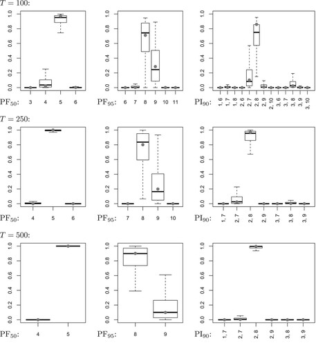
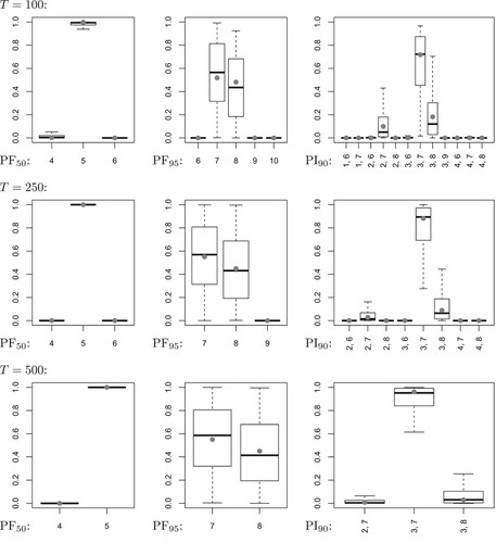
Comparing the boxplots across the different types of forecasts (so across the columns in Figure 1), it becomes clear that we have a very small resampling dispersion (‘blurredness’ of forecasts) for the median forecasts, and a rather large one for the 95%-quantile forecast. This goes along with our previous conclusions, as well as with the ones in [7]. The situation might be even worse under different model parametrizations, such as the one in Figure 2 (with $\alpha =0.75$ instead of $\alpha =0.50$). But here, it is important to note that the root cause for the large resampling dispersion of the 95%-quantile forecasts is a discreteness problem, which affects the true forecast's distribution under estimation uncertainty (nearly a 50:50 distribution on $\{7,8\}$) in the same way. For $(\mu ,\alpha )=(5,0.75)$, we have $P(X_{T+1}\le 7|X_T=5)\approx 0.951$ being very close to 0.95, such that the 95%-quantile is extremely sensitive to estimation error. In contrast, for $(\mu ,\alpha )=(5,0.50)$, we have $P(X_{T+1}\le 8|X_T=5)\approx 0.957$ being clearly larger than 0.95, such that the estimated 95%-quantiles equal the true one in the large majority of cases. In fact, this discreteness problem concerning sample quantiles is also observed in more general contexts, see [9] for further details, especially their Theorem 6. While the 95%-quantile forecasts are problematic for $(\mu ,\alpha )=(5,0.75)$, we again observe consistency for the resampling of the 90%-PIs. It is also worth pointing out that in both Figures 1 and 2, the range of resampled intervals strongly decreases with increasing T, confirming our conclusions from Table A2.

Figure 2. Poi-INAR(1) DGP with $\mu =5$, $\alpha =0.75$, and sample size T. Distribution of forecasts conditioned on value 5: conditional median (‘PF${}_{50}$’, true value: 5), 95%-quantile (‘PF${}_{95}$’, true value: 7), and limits l, u of 90%-PI (‘PI${}_{90}$’, true limits: 3, 7). Distribution under estimation uncertainty as gray dots, and boxplots of resampled distributions.

3.3. Comparison to other types of DGP

To analyze if our conclusions drawn for the case of a Poi-INAR(1) DGP transfer to other types of DGP as well, also the remaining count time series models in Appendix 1 have been considered in our simulation study. Certainly, these are (by far) not the only models for count time series, see the surveys by Weiß [24,25]. For example, there are models using different thinning operations, such as the so-called ‘NGINAR(1) model’ by Ristić et al. [19] relying on negative-binomial thinning, and there are also regression-type models for time series consisting of bounded counts, such as the so-called ‘BINARCH models’ by Ristić et al. [20]. Generally, one may also consider models with a non-linear conditional mean, although problems might occur if the log-likelihood function has multiple local maxima, such as for the minification INAR model of [1]. To not make our comparisons unnecessarily complex, we restrict to the models in Appendix 1. The model parametrizations were always chosen such that the mean μ and the ACF at lag 1, $\rho \left(1\right)=\alpha$, agree across all models. The third model parameter of the NB- and ZIP-INAR(1) model, respectively, was used to ensure that the variance-mean ratio equals ${\sigma }^2/\mu =1.5$ (i.e. 50% overdispersion). The second-order AR parameter of the Poi-INAR(2) model was uniquely chosen as ${\alpha }_2=0.25$, and we computed ${\alpha }_1=\alpha (1-{\alpha }_2)$. Here, forecasting was done conditioned on the respective last two observations $x_T,x_{T-1}$ in each Monte–Carlo run. Finally, the possible upper bounds of the BAR(1) model are $n\in \{10,20,40\}$, leading to the mean $\mu =n\pi$ with the unique choice $\pi =0.25$. The tabulated results are again collected in Appendix 2, where in each table, always one feature is compared across all types of DGP.

Table A3 provides the numbers of those simulation runs, where the respective forecast based on the estimated parameter values agrees with the one using the true parameter values. Like for the Poi-INAR(1) DGP (first block of columns in Table A3), the forecasts obtained by using estimated parameters often deviate from the true ones also for the remaining models. This deviation is particularly large for the NB- and ZIP-INAR(1) model with their additional overdispersion, and also much larger for the non-central PF and the PI than for the central PF. For the Poi-INARCH(1) DGP, these agreement numbers are more stable across different values of α than for the Poi-INAR(1) DGP. If we would take the modes of the resampled forecasts as the substitutes of the forecasts under estimation uncertainty, then nearly nothing changes because of the modes just reproducing these forecasts most of the times (Table A4).

The full set of resampled forecasts, in contrast, covers the true forecast nearly without exception (Table A5). Only in the presence of additional overdispersion (NB- or ZIP-INAR(1) model) and for the small sample size T = 100, the coverage rate might fall below 99%. Thus, the proposed resampling approach successfully accounts for the effect of parameter estimation for any of the considered DGPs. Finally, let us analyze the mean sizes of the sets of different resampled forecasts (degree of blurredness), see Table A6. For the Poi-INARCH(1) DGP, these sets typically consist of only 2–4 different forecasts in the mean. These values are more homogeneous than in the Poi-INAR(1) case, i.e. there is less difference between PFs and PIs, and less difference regarding varying values of α. The BAR(1) values resemble those of the Poi-INAR(1) DGP, and also the mean sizes for the central PF are quite similar for all types of DGP. However, the sets of the resampled non-central PFs and, in particular, those of the PIs might become quite large. This can be observed for the Poi-INAR(2) DGP with large mean μ and, in particular, for the NB- and ZIP-INAR(1) DGP (if again μ is large, and if the ACF parameter α is small). Fortunately, these mean sizes get quickly reduced for increasing sample size T. Furthermore, the resampled PIs are strongly overlapping such that a reasonable interpretation is still possible even if the number of different PIs is large. This is illustrated by the example presented in Section 4.

4. Real-data example

To illustrate the application of the resampling approach for coherent forecasting proposed in Section 2, we consider a count time series about the monthly numbers of ‘work stoppages’ (strikes and lock-outs) of $\ge 1000$ workers in the U.S. These numbers are published by the U. S. Bureau of Labor Statistics at https://www.bls.gov/wsp/. A part of these data, the T = 108 counts referring to the period 1994–2002, has already been analyzed by Jung et al. [11], Weiß [23,24] and others. It turned out that these data, which are shown in Figure 3 together with their sample ACF, are well described by a Poi-INARCH(1) model. The corresponding ML estimates (with approximate standard errors in parentheses) are obtained as ${\hat{\mu }}_{ML}\approx 4.981$ (0.593) and ${\hat{\alpha }}_{ML}\approx 0.636$ (0.081). This well-established model fit shall now be used as the base for (post hoc) forecasting the counts of the year 2003 (numbered as $t=109,\dots ,120$, and also taken from the aforementioned website). Thus, we compute the coherent forecasts (again the median as a central PF, the 95%-quantile as a non-central PF, and the 90%-PI) for $x_t$ after having observed $x_{t-1}$ for $t=109,\dots ,120$. 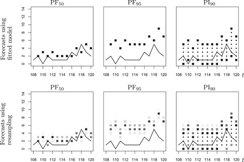If these forecasts are computed based on the estimated model, we obtain the unique forecast values shown in the upper panel of Figure 4 (to better highlight their interval nature, the interior points of the PIs are plotted with a smaller point size). This uniqueness, however, could cause the erroneous impression that these forecast values are precise.

Figure 3. Strikes counts discussed in Section 4: time series plot (left) and sample ACF with time lag k (right).

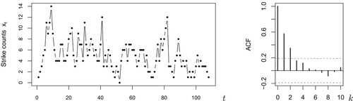
Figure 4. Strikes counts in 2003 (solid line) together with different types of forecasts: conditional median (“PF${}_{50}$”), 95%-quantile (“PF${}_{95}$”), and 90%-PI (“PI${}_{90}$”), computed from ML-estimated parameter (upper panel) or based on resampled ML-estimates (lower panel).

To account for the apparent estimation uncertainty, in the way described in Section 2, we first compute the inverse Hessian of the log-likelihood function at its maximum, i.e. at $({\hat{\mu }}_{ML},{\hat{\alpha }}_{ML})$. This is directly offered by the numerical optimization routine used for the ML computation (we used the function optim in R). It leads to the approximate bivariate normal distribution $N\left(\left(\begin{array}{c}4.981\\ 0.636\end{array}\right),\left(\begin{array}{cc}0.352& 0.016\\ 0.016& 0.007\end{array}\right)\right),$ which is used for simulating the B = 500 replicates $({\hat{\mu }}_{ML,b}^{\star },{\hat{\alpha }}_{ML,b}^{\star })$ with $b=1,\dots ,B$ (we used mvrnorm in R's MASS package). Then, for $t=109,\dots ,120$, we compute all forecasts for $x_t$ again, namely B times based on the replicates $({\hat{\mu }}_{ML,b}^{\star },{\hat{\alpha }}_{ML,b}^{\star })$. As an example, the (post hoc) forecasts for $x_{109}=2$, given that $x_{108}=1$, are (absolute frequencies shown in parentheses)

• PF${}_{50}$: 2 if using the fitted model, but 1 (6), 2 (382), 3 (112) under resampling;

• PF${}_{95}$: 5 if using the fitted model, but 4 (44), 5 (311), 6 (141), 7 (4) under resampling;

• PI${}_{90}$: $\{0,\dots ,5\}$ if using the fitted model, but $\{0,\dots ,3\}$ (12), $\{0,\dots ,4\}$ (254), $\{0,\dots ,5\}$ (207), $\{1,\dots ,6\}$ (27) under resampling.

So instead of a unique forecast value, we get 3–4 values together with their frequencies; these support lengths are plausible in view of Table A6, see the values for the Poi-INARCH(1) DGP with $\mu =5$ and T = 100. Also note that the mode of the resampled forecasts equals the forecast of the fitted model for PF${}_{50}$ and PF${}_{95}$, but slightly differs for PI${}_{90}$; recall the discussion of Table A4. The frequency distributions of the resampled PFs are easily visualized by plotting all forecasts as gray dots, where the gray levels are proportional to the respective frequencies (with black=100% and white=0%), see the first two graphs in the lower panel of Figure 4. So instead of a single dot that leads the viewer to believe in an exact inference, the blurred structure reveals the estimation uncertainty in forecasting and expresses which count values are likely to be the true PF value. Recalling Table A5, we can be rather sure that the respective true PF value is covered by the resampled ones. If, for example, some management decisions rely on PF values regarding the monthly strikes, then these should better use the information about the estimation uncertainty as resulting from resampling, e. g. by using a worst-case strategy.

For the PIs, the situation is slightly more complicated at a first glance, because there is no strict order between the computed sets. However, also recall the comment in the end of Section 3.3, the sets are strongly overlapping. We evaluated the full ensemble of four PIs at t = 109 in the following way. First, we computed the union of all PIs, leading to the set $\{0,\dots ,6\}$ in the present example. Second, for each element in this superset, we computed its absolute frequency as the number of PIs covering this element, leading to 0 (473), 1–3 (500), 4 (488), 5 (234), and 6 (27). These frequencies are then used for computing the gray levels of the dots printed at t = 109 in the last graph of Figure 4 (in addition, the interior points with absolute frequency B = 500 are again plotted with a smaller point size). Note that the superset $\{0,\dots ,6\}$ is only slightly larger than the PI $\{0,\dots ,5\}$ of the fitted model, i.e. we have an only small increase of ambiguity in this sense (similar at $t=110,\dots ,120$, see the last column in Figure 4). Furthermore, in view of our simulation results in Table A5 (see the Poi-INARCH(1) DGP with $\mu =5$ and T = 100), we can be very confident that the true 90%-PIs are covered by the resampled ones. In addition, we can see that in view of estimation uncertainty, the counts 0–4 are much more likely to be contained in the true PI than the remaining counts 5–6. This refined information is not provided the PI $\{0,\dots ,5\}$ of the fitted model.

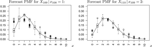
Let us conclude the data application by briefly discussing the task of ‘PMF forecasting’ mentioned in Section 1. As an intermediate step of our resampling approach, we had to compute the forecast PMF for each replicate $({\hat{\mu }}_{ML,b}^{\star },{\hat{\alpha }}_{ML,b}^{\star })$, because the PMF was used to derive the PFs and PIs. Thus, if a practitioner is interested in the full forecast PMF instead of PFs or PIs, the ensemble of B replicated forecast PMFs can be used to express the actual estimation uncertainty. This is illustrated in Figure 5, where we compare the forecast PMFs for $X_{109}|x_{108}=1$ and $X_{110}|x_{109}=2$ based on the ML-fitted model (shown as a gray line) with box plots of the B PMF values computed for $x=0,1,\dots$, respectively. The box plots clearly indicate where we have to account for how much uncertainty (in a similar spirit, Harris et al. [6] used animated graphics to visualize the effect of estimation uncertainty on forecast densities). The box plots also confirm the above PF and PI computations. For example, the left graph shows that the PMF value for the event $X_{109}=0|x_{108}=1$ is hardly below 0.05 such that the large majority of two-sided PI${}_{90}$s includes the count 0. For $X_{110}=0|x_{109}=2$ (right graph), in contrast, the median PMF value 0.047 is slightly below 0.05, and also the PI${}_{90}$ based on the ML-fitted model does not include the count 0, recall the upper-right graph in Figure 4. But the actually realized count is $x_{110}=0$, i.e. it is erroneously not covered by the fitted model's PI${}_{90}$. This problem does not occur for the resampled PI${}_{90}$ s, because 214 out of 500 include the count 0, so it is quite likely that the true PI${}_{90}$ would cover the oberserved $x_{110}=0$.

Figure 5. Forecast PMFs $P(X_{T+1}=x|x_T)$ for strikes counts in Jan./Feb. 2003, computed from ML-estimated parameter (grey line) or based on resampled ML-estimates (box plots).

5. Conclusions

To account for the estimation uncertainty in coherent forecasting of count processes, we proposed an efficient resampling scheme that relies on the asymptotic normal distribution of the DGP's ML estimator, and that generates an ensemble of forecast values instead of a single (and possibly wrong) forecast value. Our resampling approach requires much less computing than if using a traditional parametric bootstrap implementation but shows a very similar performance. It mimics the respective forecast's true sampling distribution and thus describes the actual estimation uncertainty in forecasting. The obtained ensembles of PF or PI values can be represented visually to simplify the interpretation by a practitioner. Our approach is also easily adapted to PMF forecasting. For future research, also other types of discrete-valued processes (such as ordinal processes) should be considered, and one should try to adapt the above forecasting and resampling approaches to such type of data. For count processes, in turn, the forecasting of risk is relevant in some applications. In contrast to the discrete count values themselves, common risk measures for counts are often positively real-valued. It would be interesting to study the effect of parameter estimation on risk forecasts for count processes, and to develop adequate ways of incorporating the resulting estimation uncertainty into such continuous-valued types of forecasts.

Acknowledgments

The authors thank the two referees for their useful comments on an earlier draft of this article. This research was funded by the Deutsche Forschungsgemeinschaft (DFG, German Research Foundation) – Projektnummer 394832307.

Disclosure statement

No potential conflict of interest was reported by the author(s).

Additional information

Funding

This work was supported by Deutsche Forschungsgemeinschaft [394832307].

Appendices

Appendix 1.

Summary of considered count DGPs

In what follows, we summarize those count time series models, which were used as a DGP in our simulation studies. More details and references on these and further count time series models can be found in the book by Weiß [24], or in the survey article by Weiß [25]. The INAR(1) model is defined by the recursive scheme (A1) $X_t=\alpha \circ X_{t-1}+{ϵ}_t\mathrm{w}\mathrm{i}\mathrm{t}\mathrm{h}\alpha \in (0,1),$(A1) where the innovations ${ϵ}_t$ are i. i. d. count random variables, and where ‘°’ denotes the binomial thinning operator. The latter is defined by a conditional binomial distribution, $\alpha \circ X|X\sim Bin(X,\alpha )$, and it is executed independently of the innovations and of already available observations. Important special cases are the

• Poi-INAR(1) model, where ${ϵ}_t$ follows a Poisson (Poi) distribution;

• NB-INAR(1) model, where ${ϵ}_t$ follows a negative binomial (NB) distribution;

• ZIP-INAR(1) model, where ${ϵ}_t$ follows a zero-inflated Poisson (ZIP) distribution.

With $\mu =E\left[X_t\right],{\mu }_{ϵ}=E\left[{ϵ}_t\right]$ denoting the means, ${\sigma }^2=V\left[X_t\right],{\sigma }_{ϵ}^2=V\left[{ϵ}_t\right]$ the variances, and $\rho \left(k\right)=Corr[X_t,X_{t-k}]$ the autocorrelation function (ACF), it holds that $\mu =\frac{{\mu }_{ϵ}}{1-\alpha },\frac{{\sigma }^2}{\mu }=\frac{{\sigma }_{ϵ}^2/{\mu }_{ϵ}+\alpha }{1+\alpha },\mathrm{a}\mathrm{n}\mathrm{d}\rho \left(k\right)={\alpha }^k.$ The conditional distribution of $X_t|X_{t-1}$ is a convolution of the thinning's binomial distribution, $Bin(X_{t-1},\alpha )$, and the distribution of ${ϵ}_t$. A second-order extension of (A1(A1) $X_t=\alpha \circ X_{t-1}+{ϵ}_t\mathrm{w}\mathrm{i}\mathrm{t}\mathrm{h}\alpha \in (0,1),$(A1) ), the INAR(2) model, is obtained by the recursion (A2) $X_t={\alpha }_1\circ X_{t-1}+{\alpha }_2\circ X_{t-2}+{ϵ}_t\mathrm{w}\mathrm{i}\mathrm{t}\mathrm{h}{\alpha }_1+{\alpha }_2\in (0,1),$(A2) where all thinnings are executed independently. The distribution of $X_t|X_{t-1},X_{t-2}$ is a convolution of $Bin(X_{t-1},{\alpha }_1)$, $Bin(X_{t-2},{\alpha }_2)$, and the distribution of ${ϵ}_t$. The ACF satisfies $\rho \left(1\right)={\alpha }_1/(1-{\alpha }_2)$, and $\rho \left(k\right)={\alpha }_1\rho (k-1)+{\alpha }_2\rho (k-2)$ for $k\ge 2$.

A modification of (A1(A1) $X_t=\alpha \circ X_{t-1}+{ϵ}_t\mathrm{w}\mathrm{i}\mathrm{t}\mathrm{h}\alpha \in (0,1),$(A1) ) for counts having the bounded range $\{0,\dots ,n\}$ with some $n\in \mathbb{N}$, the binomial AR(1) model, is defined by (A3) $X_t=\gamma \circ X_{t-1}+\text{β}\circ (n-X_{t-1})\mathrm{w}\mathrm{i}\mathrm{t}\mathrm{h}{X}_0\sim Bin(n,\pi ).$(A3) Here, the model parameters are $\pi \in (0,1)$ and $\alpha \in (max\{-\frac{\pi }{1-\pi },-\frac{1-\pi }{\pi }\},1)$, and we define the thinning probabilities as $\text{β}=\pi (1-\alpha )$ and $\gamma =\text{β}+\alpha$. The BAR(1) process (A3(A3) $X_t=\gamma \circ X_{t-1}+\text{β}\circ (n-X_{t-1})\mathrm{w}\mathrm{i}\mathrm{t}\mathrm{h}{X}_0\sim Bin(n,\pi ).$(A3) ) has the marginal distribution $Bin(n,\pi )$, the ACF $\rho \left(k\right)={\alpha }^k$, and the conditional distribution of $X_t|X_{t-1}$ is a convolution of $Bin(X_{t-1},\gamma )$ and $Bin(n-X_{t-1},\text{β})$.

Another modification of (A1(A1) $X_t=\alpha \circ X_{t-1}+{ϵ}_t\mathrm{w}\mathrm{i}\mathrm{t}\mathrm{h}\alpha \in (0,1),$(A1) ) is the Poi-INARCH(1) model (where ‘CH’ abbreviates ‘conditional heteroskedasticity’), which follows the recursion (A4) $X_t|X_{t-1},\dots \sim Poi(\text{β}+\alpha X_{t-1})\mathrm{w}\mathrm{i}\mathrm{t}\mathrm{h}\alpha \in (0,1)\mathrm{a}\mathrm{n}\mathrm{d}\text{β}>0.$(A4) Mean, variance, and ACF, respectively, are given by $\mu =\frac{\text{β}}{1-\alpha },\frac{{\sigma }^2}{\mu }=\frac{1}{1-{\alpha }^2},\mathrm{a}\mathrm{n}\mathrm{d}\rho \left(k\right)={\alpha }^k.$

Appendix 2.

Tables with simulation results for Section 3

Table A1. Coherent forecasting of Poi-INAR(1) DGP: conditional median (‘PF${}_{50}$’), 95%-quantile (‘PF${}_{95}$’), and 90%-PI (‘PI${}_{90}$’), computed from true parameter, ML-estimated parameter, or based on resampled ML-estimates.

						asymptotic resampling						parametric bootstrap
			agreement true vs. estimated			agreement estimated vs. resampling mode			true covered by resampling			agreement estimated vs. resampling mode			true covered by resampling
μ	α	T	PF${}_{50}$	PF${}_{95}$	PI${}_{90}$	PF${}_{50}$	PF${}_{95}$	PI${}_{90}$	PF${}_{50}$	PF${}_{95}$	PI${}_{90}$	PF${}_{50}$	PF${}_{95}$	PI${}_{90}$	PF${}_{50}$	PF${}_{95}$	PI${}_{90}$
2.5	0.25	100	827	766	703	985	968	958	999	1000	1000	989	974	969	1000	999	1000
		250	880	861	854	995	986	991	1000	1000	1000	995	985	983	1000	1000	1000
		500	919	923	912	993	994	994	1000	1000	1000	993	997	993	1000	1000	1000
2.5	0.50	100	848	789	805	990	982	974	1000	1000	1000	988	989	977	999	1000	999
		250	938	863	910	995	992	994	1000	1000	1000	999	991	994	1000	1000	1000
		500	974	887	950	997	990	995	1000	999	1000	999	993	997	1000	1000	1000
2.5	0.75	100	939	853	703	996	981	957	1000	1000	999	995	985	975	1000	1000	999
		250	957	925	815	994	991	974	1000	1000	998	994	993	977	1000	1000	999
		500	985	959	871	998	998	991	1000	1000	1000	1000	1000	991	1000	1000	1000
5	0.25	100	759	689	649	984	973	904	1000	1000	1000	988	980	914	1000	1000	1000
		250	876	797	776	992	980	961	1000	1000	1000	992	989	961	1000	1000	1000
		500	920	878	835	992	998	977	1000	999	999	996	995	977	999	1000	1000
5	0.50	100	833	734	559	988	973	944	1000	998	997	993	974	940	1000	999	997
		250	872	814	644	992	984	958	1000	1000	997	996	991	956	1000	999	996
		500	941	885	706	996	995	974	1000	1000	999	1000	996	965	1000	999	999
5	0.75	100	869	769	639	988	974	959	1000	1000	998	993	984	963	1000	1000	1000
		250	918	875	771	997	979	979	1000	999	999	997	983	978	1000	999	1000
		500	955	882	832	995	990	986	1000	1000	999	996	991	987	1000	1000	1000
10	0.25	100	678	635	520	964	949	923	998	1000	996	977	963	933	998	999	998
		250	790	734	696	990	985	964	1000	1000	999	983	987	967	999	1000	999
		500	848	812	751	987	985	983	1000	999	1000	991	987	979	1000	998	999
10	0.50	100	728	646	465	987	956	928	999	999	993	988	965	928	999	998	995
		250	820	771	615	992	981	945	999	1000	996	994	986	941	999	1000	997
		500	887	859	671	991	992	955	1000	998	999	992	990	956	1000	999	997
10	0.75	100	823	719	546	988	971	929	1000	999	995	991	983	928	999	999	998
		250	890	816	671	998	988	954	1000	1000	998	997	988	961	1000	1000	1000
		500	916	876	805	994	991	977	1000	1000	998	995	990	978	1000	1000	999

Table A2. Coherent forecasting of Poi-INAR(1) DGP based on resampled ML-estimates: conditional median (‘PF${}_{50}$’), 95%-quantile (‘PF${}_{95}$’), and 90%-PI (‘PI${}_{90}$’). Mean number of different forecasts obtained from resampling.

		$\mu =2.5$			$\mu =5$			$\mu =10$
α	T	PF${}_{50}$	PF${}_{95}$	PI${}_{90}$	PF${}_{50}$	PF${}_{95}$	PI${}_{90}$	PF${}_{50}$	PF${}_{95}$	PI${}_{90}$
0.25	100	2.22	2.83	3.62	2.77	3.38	5.12	3.45	4.14	6.19
	250	1.76	2.16	2.66	2.10	2.48	3.42	2.59	2.98	3.92
	500	1.55	1.79	2.19	1.76	2.06	2.72	2.11	2.39	2.98
0.5	100	2.09	2.60	3.92	2.54	3.15	5.29	3.12	3.82	7.72
	250	1.69	2.01	2.60	1.96	2.30	3.44	2.31	2.77	4.69
	500	1.50	1.70	1.90	1.64	1.93	2.63	1.93	2.23	3.36
0.75	100	1.64	2.31	3.38	2.05	2.60	4.80	2.50	3.16	6.90
	250	1.36	1.82	2.58	1.65	2.03	3.09	1.92	2.37	4.13
	500	1.26	1.49	2.14	1.46	1.78	2.43	1.66	1.97	3.04

Table A3. Coherent forecasting of different count DGPs: conditional median (‘PF${}_{50}$’), 95%-quantile (‘PF${}_{95}$’), and 90%-PI (‘PI${}_{90}$’), computed from true parameter, ML-estimated parameter, or based on resampled ML-estimates. Numbers of agreement of true and estimated forecasts.

DGP:			Poi-INAR(1)			Poi-INARCH(1)			NB-INAR(1) with ${\sigma }^2/\mu =1.5$			ZIP-INAR(1) with ${\sigma }^2/\mu =1.5$			Poi-INAR(2) with ${\alpha }_2=0.25$			BAR(1) with $\pi =0.25$
μ	α	T	PF${}_{50}$	PF${}_{95}$	PI${}_{90}$	PF${}_{50}$	PF${}_{95}$	PI${}_{90}$	PF${}_{50}$	PF${}_{95}$	PI${}_{90}$	PF${}_{50}$	PF${}_{95}$	PI${}_{90}$	PF${}_{50}$	PF${}_{95}$	PI${}_{90}$	PF${}_{50}$	PF${}_{95}$	PI${}_{90}$
2.5	0.25	100	827	766	703	818	746	756	807	543	615	770	714	658	819	703	629	854	834	792
		250	880	861	854	906	806	842	872	718	745	879	847	772	870	823	762	908	889	906
		500	919	923	912	926	897	898	886	787	804	931	907	841	914	851	818	953	925	966
2.5	0.5	100	848	789	805	781	766	714	784	612	659	765	689	671	797	733	707	920	867	777
		250	938	863	910	860	863	813	864	721	806	831	833	766	884	825	811	981	956	862
		500	974	887	950	918	910	878	859	825	903	871	895	813	939	886	884	997	982	914
2.5	0.75	100	939	853	703	819	720	786	932	638	653	914	696	706	823	778	677	944	866	718
		250	957	925	815	862	846	873	943	764	807	936	791	812	910	860	826	961	904	799
		500	985	959	871	919	876	918	943	813	891	953	852	863	936	882	838	975	949	832
5	0.25	100	759	689	649	762	676	655	720	492	430	732	674	515	709	644	604	792	758	644
		250	876	797	776	845	784	795	848	670	614	807	789	699	823	772	759	879	854	803
		500	920	878	835	909	848	840	891	754	696	877	839	809	894	840	828	926	903	830
5	0.5	100	833	734	559	754	674	650	789	525	458	720	661	521	735	650	580	796	793	642
		250	872	814	644	873	781	694	903	693	631	838	798	647	842	779	721	834	883	741
		500	941	885	706	954	827	742	957	788	721	902	849	730	898	852	815	877	943	752
5	0.75	100	869	769	639	769	738	704	847	607	571	841	738	611	762	708	623	901	813	718
		250	918	875	771	863	858	787	901	737	716	893	812	747	853	830	759	921	883	830
		500	955	882	832	930	936	877	938	820	790	905	858	798	910	894	799	936	924	865
10	0.25	100	678	635	520	686	563	616	609	382	255	690	633	164	586	540	480	743	672	653
		250	790	734	696	790	727	715	763	575	446	814	785	303	762	712	690	808	822	755
		500	848	812	751	860	804	790	853	684	568	838	822	409	844	773	733	917	877	847
10	0.5	100	728	646	465	649	587	592	691	440	313	677	618	343	607	551	477	724	687	532
		250	820	771	615	808	714	688	809	609	473	808	753	535	771	692	677	815	809	660
		500	887	859	671	879	795	703	887	706	597	841	826	689	844	813	771	836	824	705
10	0.75	100	823	719	546	673	517	614	761	535	451	693	643	486	681	596	487	824	757	556
		250	890	816	671	804	610	786	857	676	620	832	790	675	814	777	625	885	852	649
		500	916	876	805	870	680	855	906	775	732	864	852	790	870	815	745	895	899	722

Table A4. Coherent forecasting of different count DGPs: conditional median (‘PF${}_{50}$’), 95%-quantile (‘PF${}_{95}$’), and 90%-PI (‘PI${}_{90}$’), computed from true parameter, ML-estimated parameter, or based on resampled ML-estimates. Numbers of agreement of estimated forecasts and modes of resampled forecasts.

DGP:			Poi-INAR(1)			Poi-INARCH(1)			NB-INAR(1) with ${\sigma }^2/\mu =1.5$			ZIP-INAR(1) with ${\sigma }^2/\mu =1.5$			Poi-INAR(2) with ${\alpha }_2=0.25$			BAR(1) with $\pi =0.25$
μ	α	T	PF${}_{50}$	PF${}_{95}$	PI${}_{90}$	PF${}_{50}$	PF${}_{95}$	PI${}_{90}$	PF${}_{50}$	PF${}_{95}$	PI${}_{90}$	PF${}_{50}$	PF${}_{95}$	PI${}_{90}$	PF${}_{50}$	PF${}_{95}$	PI${}_{90}$	PF${}_{50}$	PF${}_{95}$	PI${}_{90}$
2.5	0.25	100	985	968	958	989	979	973	983	959	947	982	975	965	979	953	921	989	986	974
		250	995	986	991	990	989	991	995	972	983	992	986	989	994	986	963	995	992	989
		500	993	994	994	997	995	992	994	989	986	993	994	995	994	985	978	994	992	997
2.5	0.5	100	990	982	974	983	988	969	985	944	946	990	977	958	980	942	919	986	982	979
		250	995	992	994	992	992	990	986	983	969	990	988	982	991	977	989	995	995	989
		500	997	990	995	993	993	990	987	981	988	996	992	990	998	993	984	1000	1000	997
2.5	0.75	100	996	981	957	976	951	943	994	943	925	994	962	962	978	948	917	996	978	975
		250	994	991	974	985	977	990	997	973	967	998	981	975	995	978	969	997	990	988
		500	998	998	991	994	986	987	996	986	994	995	986	978	992	989	973	1000	996	994
5	0.25	100	984	973	904	980	971	922	980	952	902	984	977	916	967	960	908	986	980	969
		250	992	980	961	991	988	986	982	982	956	989	988	966	991	976	971	991	990	987
		500	992	998	977	995	993	995	993	989	969	992	991	984	990	987	985	993	986	995
5	0.5	100	988	973	944	971	967	932	983	921	891	971	981	914	968	943	887	988	982	969
		250	992	984	958	986	992	977	990	976	956	984	989	968	994	975	939	992	987	974
		500	996	995	974	995	990	988	997	987	973	983	987	975	993	986	978	993	997	978
5	0.75	100	988	974	959	967	958	919	988	946	925	988	980	943	974	931	903	994	976	968
		250	997	979	979	980	984	970	988	976	963	988	993	978	987	980	966	999	989	987
		500	995	990	986	991	990	983	996	991	986	996	995	985	995	977	976	997	989	995
10	0.25	100	964	949	923	970	951	900	966	911	833	980	972	701	939	920	858	977	967	947
		250	990	985	964	983	986	967	980	956	899	989	991	806	982	963	939	988	986	975
		500	987	985	983	993	992	981	990	985	939	994	992	875	993	982	970	998	991	982
10	0.5	100	987	956	928	972	944	886	969	902	810	973	956	824	959	903	857	984	977	917
		250	992	981	945	986	981	971	979	952	908	990	991	910	979	965	935	985	984	962
		500	991	992	955	992	986	978	993	972	941	989	992	954	991	989	965	989	988	971
10	0.75	100	988	971	929	945	918	899	977	926	859	972	957	888	957	891	866	984	976	931
		250	998	988	954	982	982	965	988	972	932	983	983	946	976	970	937	997	989	965
		500	994	991	977	995	979	982	997	983	956	992	992	968	989	976	965	995	993	977

Table A5. Coherent forecasting of different count DGPs: conditional median (‘PF${}_{50}$’), 95%-quantile (‘PF${}_{95}$’), and 90%-PI (‘PI${}_{90}$’), computed from true parameter, ML-estimated parameter, or based on resampled ML-estimates. Numbers of cases, where true forecasts covered by resampled forecasts.

DGP:			Poi-INAR(1)			Poi-INARCH(1)			NB-INAR(1) with ${\sigma }^2/\mu =1.5$			ZIP-INAR(1) with ${\sigma }^2/\mu =1.5$			Poi-INAR(2) with ${\alpha }_2=0.25$			BAR(1) with $\pi =0.25$
μ	α	T	PF${}_{50}$	PF${}_{95}$	PI${}_{90}$	PF${}_{50}$	PF${}_{95}$	PI${}_{90}$	PF${}_{50}$	PF${}_{95}$	PI${}_{90}$	PF${}_{50}$	PF${}_{95}$	PI${}_{90}$	PF${}_{50}$	PF${}_{95}$	PI${}_{90}$	PF${}_{50}$	PF${}_{95}$	PI${}_{90}$
2.5	0.25	100	999	1000	1000	1000	1000	1000	1000	996	995	998	1000	999	1000	999	992	999	1000	1000
		250	1000	1000	1000	1000	999	1000	999	1000	1000	1000	1000	999	1000	1000	999	1000	1000	1000
		500	1000	1000	1000	1000	999	1000	1000	998	998	1000	1000	1000	1000	999	1000	1000	1000	1000
2.5	0.5	100	1000	1000	1000	999	1000	999	1000	996	999	998	999	998	1000	999	999	1000	1000	1000
		250	1000	1000	1000	1000	1000	1000	1000	997	1000	1000	999	1000	1000	998	1000	1000	1000	1000
		500	1000	999	1000	999	999	1000	1000	999	1000	1000	999	1000	1000	1000	1000	1000	1000	1000
2.5	0.75	100	1000	1000	999	1000	999	1000	1000	993	999	999	997	999	999	998	999	1000	999	999
		250	1000	1000	998	1000	1000	1000	1000	999	998	999	999	1000	1000	1000	999	1000	1000	1000
		500	1000	1000	1000	1000	999	1000	1000	1000	996	1000	1000	1000	999	1000	1000	1000	1000	1000
5	0.25	100	1000	1000	1000	998	999	1000	1000	993	990	999	999	994	1000	999	1000	1000	1000	1000
		250	1000	1000	1000	1000	998	999	999	999	1000	999	1000	1000	1000	999	1000	1000	1000	999
		500	1000	999	999	1000	1000	1000	1000	999	999	999	1000	1000	1000	1000	1000	1000	1000	1000
5	0.5	100	1000	998	997	999	998	999	999	996	994	999	995	993	1000	995	994	1000	999	997
		250	1000	1000	997	999	999	998	1000	1000	999	1000	1000	997	998	999	998	1000	1000	997
		500	1000	1000	999	1000	1000	1000	1000	1000	1000	1000	1000	998	1000	998	1000	999	1000	1000
5	0.75	100	1000	1000	998	999	1000	999	1000	996	998	996	996	996	1000	999	998	1000	1000	998
		250	1000	999	999	1000	1000	1000	1000	998	997	1000	1000	999	998	999	999	1000	1000	999
		500	1000	1000	999	1000	1000	999	1000	1000	999	1000	1000	996	1000	1000	997	1000	1000	999
10	0.25	100	998	1000	996	1000	1000	1000	999	991	987	998	996	951	1000	1000	997	999	999	998
		250	1000	1000	999	999	999	1000	1000	1000	996	1000	1000	991	998	1000	997	1000	1000	1000
		500	1000	999	1000	1000	1000	1000	1000	1000	1000	1000	1000	993	999	1000	1000	1000	1000	999
10	0.5	100	999	999	993	1000	999	998	1000	1000	992	991	991	982	1000	999	998	1000	999	997
		250	999	1000	996	999	1000	999	1000	998	999	998	1000	995	999	999	1000	1000	1000	999
		500	1000	998	999	1000	1000	998	1000	1000	997	1000	1000	1000	999	998	999	1000	1000	1000
10	0.75	100	1000	999	995	995	996	996	999	997	994	987	979	970	1000	1000	998	999	1000	995
		250	1000	1000	998	1000	998	1000	1000	999	999	997	997	998	1000	998	998	1000	1000	997
		500	1000	1000	998	1000	1000	1000	1000	1000	1000	1000	1000	1000	1000	999	998	1000	1000	1000

Table A6. Coherent forecasting of different count DGPs: conditional median (‘PF${}_{50}$’), 95%-quantile (‘PF${}_{95}$’), and 90%-PI (‘PI${}_{90}$’), computed from true parameter, ML-estimated parameter, or based on resampled ML-estimates. Mean lengths of support of resampled forecasts.

DGP:			Poi-INAR(1)			Poi-INARCH(1)			NB-INAR(1) with ${\sigma }^2/\mu =1.5$			ZIP-INAR(1) with ${\sigma }^2/\mu =1.5$			Poi-INAR(2) with ${\alpha }_2=0.25$			BAR(1) with $\pi =0.25$
μ	α	T	PF${}_{50}$	PF${}_{95}$	PI${}_{90}$	PF${}_{50}$	PF${}_{95}$	PI${}_{90}$	PF${}_{50}$	PF${}_{95}$	PI${}_{90}$	PF${}_{50}$	PF${}_{95}$	PI${}_{90}$	PF${}_{50}$	PF${}_{95}$	PI${}_{90}$	PF${}_{50}$	PF${}_{95}$	PI${}_{90}$
2.5	0.25	100	2.22	2.83	3.62	2.27	2.98	3.04	2.53	4.18	4.51	2.72	3.28	3.94	2.50	3.20	4.34	2.15	2.32	3.04
		250	1.76	2.16	2.66	1.82	2.24	2.34	1.90	3.10	3.11	2.13	2.45	2.71	1.95	2.36	3.06	1.81	1.82	2.32
		500	1.55	1.79	2.19	1.56	1.88	1.95	1.67	2.46	2.43	1.77	2.02	2.07	1.67	1.98	2.45	1.54	1.61	1.89
2.5	0.5	100	2.09	2.60	3.92	2.39	3.13	3.09	2.29	3.95	4.85	2.40	3.28	4.55	2.47	3.10	4.50	2.01	2.26	3.45
		250	1.69	2.01	2.60	1.82	2.23	2.32	1.75	2.93	3.22	1.83	2.39	2.97	1.88	2.27	2.88	1.62	1.82	2.32
		500	1.50	1.70	1.90	1.58	1.83	1.95	1.61	2.39	2.55	1.64	2.01	2.32	1.63	1.89	2.07	1.37	1.49	1.78
2.5	0.75	100	1.64	2.31	3.38	2.40	3.25	3.17	1.70	3.65	4.54	1.67	3.41	4.82	2.31	3.02	4.64	1.55	2.03	2.83
		250	1.36	1.82	2.58	1.85	2.37	2.21	1.39	2.67	3.17	1.38	2.41	3.17	1.74	2.15	2.94	1.30	1.72	2.28
		500	1.26	1.49	2.14	1.59	1.99	1.66	1.21	2.16	2.49	1.20	2.03	2.38	1.53	1.75	2.30	1.22	1.54	1.97
5	0.25	100	2.77	3.38	5.12	2.87	3.57	3.62	3.12	4.95	9.03	3.14	3.65	8.15	3.07	3.81	6.00	2.54	2.85	3.90
		250	2.10	2.48	3.42	2.18	2.62	2.72	2.38	3.59	5.68	2.28	2.60	4.90	2.37	2.77	3.64	1.93	2.16	2.64
		500	1.76	2.06	2.72	1.83	2.15	2.22	2.00	2.84	3.95	1.92	2.17	3.41	1.93	2.24	2.55	1.65	1.80	2.19
5	0.5	100	2.54	3.15	5.29	2.94	3.65	3.67	2.88	4.65	8.10	3.09	3.60	7.27	3.07	3.78	6.40	2.33	2.72	4.55
		250	1.96	2.30	3.44	2.21	2.63	2.65	2.16	3.39	5.00	2.33	2.58	4.35	2.27	2.67	3.85	1.79	2.02	2.90
		500	1.64	1.93	2.63	1.86	2.14	2.04	1.85	2.72	3.50	1.95	2.12	3.05	1.88	2.13	2.87	1.58	1.76	2.22
5	0.75	100	2.05	2.60	4.80	2.97	3.70	3.73	2.20	4.09	6.57	2.27	3.36	5.91	2.80	3.57	6.58	1.89	2.36	4.26
		250	1.65	2.03	3.09	2.23	2.63	2.74	1.76	3.00	4.00	1.79	2.48	3.71	2.09	2.49	3.84	1.57	1.80	2.82
		500	1.46	1.78	2.43	1.82	2.10	2.11	1.55	2.45	3.01	1.58	2.06	2.67	1.74	2.02	2.83	1.40	1.58	2.13
10	0.25	100	3.45	4.14	6.19	3.55	4.25	4.23	4.05	6.15	15.77	3.56	4.04	18.20	3.97	4.70	8.39	3.18	3.51	5.48
		250	2.59	2.98	3.92	2.67	3.11	3.00	2.92	4.37	9.23	2.63	2.94	11.65	2.88	3.33	4.91	2.36	2.58	3.47
		500	2.11	2.39	2.98	2.21	2.48	2.45	2.38	3.38	6.17	2.13	2.34	8.37	2.35	2.68	3.55	1.95	2.11	2.54
10	0.5	100	3.12	3.82	7.72	3.74	4.49	4.50	3.75	5.76	13.68	3.63	4.05	13.00	3.88	4.66	9.60	2.86	3.29	6.48
		250	2.31	2.77	4.69	2.68	3.12	3.16	2.73	4.09	7.96	2.63	2.89	7.47	2.80	3.26	5.38	2.14	2.42	4.13
		500	1.93	2.23	3.36	2.19	2.47	2.49	2.18	3.18	5.30	2.11	2.33	5.05	2.26	2.56	3.76	1.76	1.97	3.04
10	0.75	100	2.50	3.16	6.90	3.80	4.53	4.68	2.92	4.84	9.98	3.04	3.77	8.66	3.69	4.57	10.22	2.33	2.84	5.86
		250	1.92	2.37	4.13	2.67	3.04	3.19	2.14	3.50	5.74	2.37	2.71	5.12	2.55	3.02	5.44	1.80	2.15	3.63
		500	1.66	1.97	3.04	2.14	2.43	2.53	1.82	2.78	4.07	1.99	2.19	3.60	2.05	2.33	3.73	1.56	1.79	2.76

References

- M.S. Aleksić and M.M. Ristić, A geometric minification integer-valued autoregressive model, Appl. Math. Model. 90 (2021), pp. 265–280.
- P. Billingsley, Statistical Inference for Markov Processes, University of Chicago Press, Chicago, 1961.
- L. Bisaglia and M. Gerolimetto, Forecasting integer autoregressive processes of order 1: are simple AR competitive? Econ. Bulletin 35 (2015), pp. 1652–1660.
- R. Bu, B. McCabe, and K. Hadri, Maximum likelihood estimation of higher-order integer-valued autoregressive processes, Journal of Time Series Analysis 29 (2008), pp. 973–994.
- R.K. Freeland and B.P.M. McCabe, Forecasting discrete valued low count time series, Int. J. Forecast. 20 (2004), pp. 427–434.
- D. Harris, G.M. Martin, I. Perera, and D.S. Poskitt, Construction and visualization of confidence sets for frequentist distributional forecasts, J. Comput. Graph. Stat. 28 (2019), pp. 92–104.
- A. Homburg, C.H. Weiß, L.C. Alwan, G. Frahm, and R. Göb, Evaluating approximate point forecasting of count processes, Econometrics 7 (2019), 30.
- A. Homburg, C.H. Weiß, L.C. Alwan, G. Frahm, and R. Göb, A performance analysis of prediction intervals for count time series, J. Forecasting. 2020. https://doi.org/https://doi.org/10.1002/for.2729.
- C. Jentsch and A. Leucht, Bootstrapping sample quantiles of discrete data, Ann. Inst. Stat. Math. 68 (2016), pp. 491–539.
- C. Jentsch and C.H. Weiß, Bootstrapping INAR models, Bernoulli 25 (2019), pp. 2359–2408.
- R.C. Jung, G. Ronning, and A.R. Tremayne, Estimation in conditional first order autoregression with discrete support, Stat. Papers 46 (2005), pp. 195–224.
- R.C. Jung and A.R. Tremayne, Coherent forecasting in integer time series models, Int. J. Forecast. 22 (2006), pp. 223–238.
- D.R. Kim and S.Y. Hwang, Forecasting evaluation via parametric bootstrap for threshold-INARCH models, Commun. Stat. Appl. Methods. 27 (2020), pp. 177–187.
- S. Kolassa, Evaluating predictive count data distributions in retail sales forecasting, Int. J. Forecast. 32 (2016), pp. 788–803.
- J.-P. Kreiß and E. Paparoditis, Bootstrap methods for dependent data: A review, J. Korean. Stat. Soc. 40 (2011), pp. 357–378.
- B.P.M. McCabe and G.M. Martin, Bayesian predictions of low count time series, Int. J. Forecast. 21 (2005), pp. 315–330.
- B.P.M. McCabe, G.M. Martin, and D. Harris, Efficient probabilistic forecasts for counts, J. R. Statist. Soc. – Ser. B 73 (2011), pp. 253–272.
- T.N. Palmer, The economic value of ensemble forecasts as a tool for risk assessment: from days to decades, Q. J. R. Meteorolog. Soc. 128 (2002), pp. 747–774.
- M.M. Ristić, H.S. Bakouch, and A.S. Nastić, A new geometric first-order integer-valued autoregressive (NGINAR(1)) process, J. Stat. Plan. Inference. 139 (2009), pp. 2218–2226.
- M.M. Ristić, C.H. Weiß, and A.D. Janjić, A binomial integer-valued ARCH model, Int. J. Biostatist. 12 (2016), 20150051.
- N. Silva, I. Pereira, and M.E. Silva, Forecasting in INAR(1) model, REVSTAT 24 (2009), pp. 171–176.
- R.D. Snyder, J.K. Ord, and A. Beaumont, Forecasting the intermittent demand for slow-moving inventories: A modelling approach, Int. J. Forecast. 28 (2012), pp. 485–496.
- C.H. Weiß, The INARCH(1) model for overdispersed time series of counts, Commun. Statist. – Simul. Comput. 39 (2010), pp. 1269–1291.
- C.H. Weiß, An Introduction to Discrete-Valued Time Series, John Wiley & Sons Inc., Chichester, 2018.
- C.H. Weiß, Stationary count time series models, WIREs Comput. Stat. 13 (2021), e1502.
- T.R. Willemain, C.N. Smart, and H.F. Schwarz, A new approach to forecasting intermittent demand for service parts inventories, Int. J. Forecast. 20 (2004), pp. 375–387.