Model averaging in calibration of near-infrared instruments with correlated high-dimensional data

Abstract

Model averaging (MA) is a modelling strategy where the uncertainty in the configuration of selected variables is taken into account by weight-combining each estimate of the so-called ‘candidate model’. Some studies have shown that MA enables better prediction, even in high-dimensional cases. However, little is known about the model prediction performance at different types of multicollinearity in high-dimensional data. Motivated by calibration of near-infrared (NIR) instruments,we focus on MA prediction performance in such data. The weighting schemes that we consider are based on the Akaike’s information criterion (AIC), Mallows’ C_p, and cross-validation. For estimating the model parameters, we consider the standard least squares and the ridge regression methods. The results indicate that MA outperforms model selection methods such as LASSO and SCAD in high-correlation data. The use of Mallows’ C_p and cross-validation for the weights tends to yield similar results in all structures of correlation, although the former is generally preferred. We also find that the ridge model averaging outperforms the least-squares model averaging. This research suggests ridge model averaging to build a relatively better prediction of the NIR calibration model.

Keywords:

• Model averaging
• high-dimensional data
• multicollinearity
• calibration
• near-infrared spectroscopy

1. Introduction

In a calibration of near-infrared (NIR) instruments, we model the concentrations of chemical compositions as a function of their NIR spectra measured at hundreds or thousands of wavelengths [8]. The main objective of the calibration is to build a model with the best prediction. The spectra data are generally known to have some characteristics that pose a challenge in the modelling: first, the number of variables (wavelengths) far exceeds the number of observations and, second, the variables are highly correlated. When facing these challenges in the modelling, we usually consider a variable selection or model selection method. Some candidate models with different configurations of variables are identified first. One may then consider forward selection, backward selection, Akaike's information criterion (AIC), Mallows' $C_p$, or cross validation (CV), to arrive at the ‘best’ model. Rather than focusing only on the ‘best’ model, a different approach called model averaging (MA) has been proposed to consider all candidate models. These candidate models are constructed by different subsets of predictors. The prediction is performed by combining predictions from these candidate models, in which higher weights are given to better models. In effect, the configuration of variables is taken into account in the prediction [6]. This MA approach has also been shown to have a good prediction, even in the case of high-dimensional data [2]. We know little, however, whether MA would be advantageous for prediction in the case of high-dimensional and highly correlated data such as the context of a calibration of NIR instruments. Therefore, this study investigates the prediction performance of MA in such a situation and compares it with MA in data with low correlation and ‘block’ correlation within a simulation study.

Just like in any general statistical modelling, there are two main approaches to MA that reflect different schools of thought: Bayesian model averaging (BMA) and frequentist model averaging (FMA). In BMA, we require a prior distribution and compute the posterior probability of each candidate model and use them as weights in the averaging [6,12,15]. On the other hand, the FMA does not require any prior assumption and fully depends on the considered data. Its result, however, is mainly determined by (1) the procedure to construct candidate models, (2) the method to estimate model parameters, and (3) the calculation of weight (for each candidate model). This study focuses only on the FMA and the context is only on high-dimensional data.

With regard to the calculation of candidate model weights, some proposals have been put forward. Buckland et al. [3] proposed the use of the Akaike's information criterion (AIC). Hansen [9] proposed Mallows' $C_p$ and Hansen & Racine [10] later suggested the use of cross-validation (CV) criterion (jackknife MA) for the weights. For the procedure to construct candidate models, Salaki et al. [16] proposed a random partition to select the variables into candidate models. Hansen [9] and Hansen and Racine [10] proposed a nested model set-up, while Ando and Li [2] proposed a marginal correlation of covariate with response variable to construct candidate models. Magnus et al. [13] proposed a separation of focus variables, the ones that must be included in each candidate model, from auxiliary variables in the construction. With the exception of Salaki et al. [16], Zhao et al. [20], and Ando and Li [2], many of literatures do not specifically focus on high-dimensional data when proposing methods for candidate model construction. This point is critical to note since this is related to the methods to estimate model parameters. Unfortunately, most studies restrict themselves to use ordinary least squares (OLS) to estimate model parameters (e.g. [2,10]) even in the context of high-dimensional data. It is well known that OLS estimates tend to be unstable in the presence of correlation between variables and this could negatively affect the model prediction.

The objective of this study is to investigate how the method to calculate weights of candidate models and the method of parameter estimation affect the prediction performance of MA in modelling high-dimensional data containing different correlation structures: high correlation, low correlation, and ‘blocks’ correlation. We consider three different methods to calculate the weights of candidate models: AIC, Mallows' $C_p$, and cross validation. For the method to estimate model parameters, we consider both the OLS method and ridge method [11]. Ridge regression is considered to specifically deal with the problem of (high) multicollinearity between variables such as the case in our application. For the method to construct the candidate models, we only consider the marginal correlation between the response variable and predictors as previously done by Ando and Li [2]. They reported that this method to construct candidate models produced better prediction power compared to other methods.

We compare the model performance of MA in the above different situations with those of model selection methods: least absolute shrinkage and selection operators (LASSO) [17] and smoothly clipped absolute deviation (SCAD) [7]. These methods are known and widely used to perform variable selection and parameter estimation simultaneously by imposing a certain penalty on a model fitting criterion. Our simulation study indicates that the prediction performance of MA is determined by the correlation structure of the data, method of parameter estimation, and the calculation method for the weights. In general, we find that MA works better than penalised regression methods in high-dimensional and highly correlated data. In terms of the method of parameter estimation, we also find that ridge regression MA outperforms the least-squares MA as the candidate models contain a larger number of predictors.

The rest of this paper is organised as follows. Section 2 describes the methodology of this study. A simulation study to assess prediction performance of MA in different settings is presented in Section 3, meanwhile, Section 4 describes the results. Section 5 presents the discussion and concluding remarks of this study.

2. Methods

In this section, we describe the MA methodology. Specifically, the setting and notation of the relevant models are defined in Section 2.2. Section 2.3 outlines the MA framework with several different weighting schemes and methods of parameter estimation. However, first, we shall describe the NIR calibration dataset that motivated our study.

2.1. NIR calibration dataset

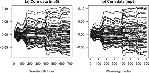
In this study, we consider two real datasets on the calibration of near-infrared spectrometer. The datasets are spectra from 80 corn specimens measured on two different spectrometers (mp5 and mp6) at 700 wavelengths between 1100 and 2496 nm in 2 nm intervals. Each spectrometer generates a spectra matrix of size 80 × 700. From each corn specimen, moisture, oil, protein and starch concentrations are measured. The average correlation between variables in the corn mp5 and mp6 datasets are 0.997 and 0.982, respectively. The datasets are originally available from http://www.eigenvector.com [1] and the spectra data are presented in Figure 1(a ,b).

Figure 1. The spectra data involved in this study: (a) corn data using mp5 spectrometer, (b) corn data using mp6 spectrometer. The scale on vertical axis is arbitrary. The lines connect the absorbances of the same experimental specimen across different wavelengths. See the main text in Section 2.1 for more details.

2.2. Models and notation

Let $\mathbf{y}\equiv (y_1,y_2,\dots ,y_n{)}^T$ be a vector of response variable, where n is the number of observations and ‘T’ denotes transposition. Let ${\mathbf{x}}_1,{\mathbf{x}}_2,\dots ,{\mathbf{x}}_p$ be vectors of predictors, each of which is an n-vector, and let ${\text{β}}_1,{\text{β}}_2,\dots ,{\text{β}}_p$ be the corresponding model parameters, respectively. The predictors can be summarised in a matrix of predictors $\mathbf{X}$ of size $n\times p$, where of p (the number of predictors) is allowed to exceed n. Consider a linear regression model (1) $\mathbf{y}=\sum _{j=1}^p{\text{β}}_j{\mathbf{x}}_j+\mathit{ϵ}$(1) where $\text{β}\equiv \left\{{\text{β}}_j\right\}$ is a p-vector of unknown regression model parameters, $\mathit{ϵ}$ is an n-vector of random error term. We assume that ${ϵ}_i$ independently follows a normal distribution with mean zero and variance ${\sigma }^2>0$, for $i=1,2,\dots ,n$. Without loss of generality, we assume that all the variables are centred to have zero mean so that we do not need to worry about the intercept. The objective of model fitting is to estimate ${\text{β}}_1,\dots ,{\text{β}}_p$, not only for interpreting the relationship between each predictor and the response variable but also for prediction of future observations.

In the ordinary least-squares (OLS) method, $\text{β}$ is estimated as (2) ${\widehat{\text{β}}}_{\mathrm{OLS}}=\arg \mathrm{mi}{n}_{\text{β}}\left\{\right(\mathbf{y}-\mathbf{X}\text{β}{)}^T(\mathbf{y}-\mathbf{X}\text{β})\}$(2) which is given by (3) ${\widehat{\text{β}}}_{\mathrm{OLS}}=({\mathbf{X}}^T\mathbf{X}{)}^{-1}{\mathbf{X}}^T\mathbf{y}.$(3) When n<p, Equation (2(2) ${\widehat{\text{β}}}_{\mathrm{OLS}}=\arg \mathrm{mi}{n}_{\text{β}}\left\{\right(\mathbf{y}-\mathbf{X}\text{β}{)}^T(\mathbf{y}-\mathbf{X}\text{β})\}$(2) ) is over-parameterised and the estimates in Equation (3(3) ${\widehat{\text{β}}}_{\mathrm{OLS}}=({\mathbf{X}}^T\mathbf{X}{)}^{-1}{\mathbf{X}}^T\mathbf{y}.$(3) ) are not attainable. Even when n>p, the estimates in Equation (3(3) ${\widehat{\text{β}}}_{\mathrm{OLS}}=({\mathbf{X}}^T\mathbf{X}{)}^{-1}{\mathbf{X}}^T\mathbf{y}.$(3) ) tend to be unstable when high multicollinearity is present in $\mathit{X}$. To deal with this problem, we usually moderate the objective function in Equation (2(2) ${\widehat{\text{β}}}_{\mathrm{OLS}}=\arg \mathrm{mi}{n}_{\text{β}}\left\{\right(\mathbf{y}-\mathbf{X}\text{β}{)}^T(\mathbf{y}-\mathbf{X}\text{β})\}$(2) ) with a penalty function $p_{\lambda }(\cdot )$: (4) $(\mathbf{y}-\mathbf{X}\text{β}{)}^T(\mathbf{y}-\mathbf{X}\text{β})+p_{\lambda }({\text{β}}_1,\dots ,{\text{β}}_p)$(4) for some ‘tuning’ parameter $\lambda >0$. Different penalty function $p_{\lambda }$ will arrive at different solutions for $\text{β}$. In the ridge regression (RR), the estimates ${\widehat{\text{β}}}_{\mathrm{RR}}$ can be obtained by setting $p_{\lambda }({\text{β}}_1,\dots ,{\text{β}}_p)=\lambda \sum _{j=1}^p{\text{β}}_j^2$. It can be shown that the estimates can be written as (5) ${\widehat{\text{β}}}_{\mathrm{RR}}=({\mathbf{X}}^T\mathbf{X}+\lambda \mathit{R}{)}^{-1}{\mathbf{X}}^T\mathbf{y}$(5) where $\mathit{R}$ is the identity matrix of the appropriate size. Equation (5(5) ${\widehat{\text{β}}}_{\mathrm{RR}}=({\mathbf{X}}^T\mathbf{X}+\lambda \mathit{R}{)}^{-1}{\mathbf{X}}^T\mathbf{y}$(5) ) indicates that the estimates ${\widehat{\text{β}}}_{\mathrm{RR}}$ are shrunk towards zero compared to ${\widehat{\text{β}}}_{\mathrm{OLS}}$ and the amount of shrinkage depends on λ.

In the context of model selection, we can consider the penalty function such that some of the estimates of ${\text{β}}_1,{\text{β}}_2,\dots ,{\text{β}}_p$ are estimated to be zero. In effect, a variable selection is performed by negating the contribution of some variables in the prediction. As a comparison to the MA framework, we consider LASSO [17,18], Adaptive LASSO [21], MCP [19], SCAD [7], and Elastic Net [22] to represent model selection methods, although we illustrate here the penalty functions for LASSO and SCAD. To get an estimate based on LASSO, the penalty function is defined as $p_{\lambda }({\text{β}}_1,\dots ,{\text{β}}_p)=\lambda \sum _{j=1}^p|{\text{β}}_j|$. This penalty function produces a sparse solution, i.e. some of the parameters are estimated to be zero while the others are estimated to be away from zero. To get estimates based on SCAD, the penalty function is defined such that the first derivative (with regard to $\text{β}$) is given by $p_{\lambda }^{\prime }\left(\text{β}\right)=\lambda \left\{I\right(\text{β}\le \lambda )+\frac{(\mathrm{a\lambda }-\text{β}{)}_{+}}{(a-1)\lambda }I(\text{β}\ge \lambda \left)\right\}$ for some a>2, where $p_{\lambda }\left(0\right)=0$, and $I(\cdot )$ is an indicator function that equals one if the condition inside the brackets is true and zero otherwise. In our study, the parameter λ in these different estimation methods is estimated using a cross-validation method.

2.3. Model averaging

In this section, we now describe the MA methodology that we consider for our calibration problem. Consider the linear regression model in Equation (1(1) $\mathbf{y}=\sum _{j=1}^p{\text{β}}_j{\mathbf{x}}_j+\mathit{ϵ}$(1) ) and the set of predictors $\{{\mathbf{x}}_1,{\mathbf{x}}_2,\dots ,{\mathbf{x}}_p\}$ that is partitioned into K subsets (described in Section 2.3.1 below). For $k=1,2,\dots ,K$, the k-th subset of predictors is considered to construct the design matrix ${\mathbf{X}}_{\left(k\right)}$ of the k-th candidate model $M_k$. The k-th candidate model $M_k$ can be written as (6) $M_k:\mathbf{y}={\mathbf{X}}_{\left(k\right)}{\text{β}}_{\left(k\right)}+{\mathit{ϵ}}_{\left(k\right)}$(6) where ${\mathbf{X}}_{\left(k\right)}$ is a matrix of predictors of size $n\times p_{\left(k\right)}$, ${\text{β}}_{\left(k\right)}$ is a $p_{\left(k\right)}$-vector of model parameters associated with ${\mathbf{X}}_{\left(k\right)}$, and ${\mathit{ϵ}}_{\left(k\right)}$ is the random error term. The model parameters ${\text{β}}_{\left(k\right)}$ are estimated according to different estimation methods as described in Section 2.3.2 below.

Once we obtain the estimates ${\widehat{\text{β}}}_{\left(k\right)}$, we define ${\hat{\mathbf{y}}}_{\left(k\right)}$ as a fitted vector based on model $M_k$, i.e. ${\hat{\mathbf{y}}}_{\left(k\right)}={\mathbf{X}}_{\left(k\right)}{\widehat{\text{β}}}_{\left(k\right)}$. The fitted vector for MA, ${\hat{\mathbf{y}}}_{\mathrm{MA}}$, in model (1(1) $\mathbf{y}=\sum _{j=1}^p{\text{β}}_j{\mathbf{x}}_j+\mathit{ϵ}$(1) ) can be written as (7) ${\hat{\mathbf{y}}}_{\mathrm{MA}}=\sum _{k=1}^K{w}_k{\hat{\mathbf{y}}}_{\left(k\right)},$(7) where $w_k$ is the weight corresponding to the k-th candidate model, $0\le w_k\le 1\mathrm{\forall k}$ and $\sum _{k=1}^K{w}_k=1$, and is described below in Section 2.3.3. The MA parameter estimate for ${\text{β}}_j,j=1,\dots ,p$, of Equation (1(1) $\mathbf{y}=\sum _{j=1}^p{\text{β}}_j{\mathbf{x}}_j+\mathit{ϵ}$(1) ) is calculated by (8) ${\widehat{\text{β}}}_j=\sum _{k=1}^K{w}_k{\widehat{\text{β}}}_{j,\left(k\right)},$(8) where ${\widehat{\text{β}}}_{j,\left(k\right)}$ is the estimate of ${\text{β}}_j$ based on the k-th candidate model. Note that, if predictor j is not in the candidate model k, then ${\widehat{\text{β}}}_{j,\left(k\right)}=0$ for $j=1,2,\dots ,p,$ and $k=1,2,\dots ,K$.

2.3.1. Model construction

To construct the candidate models, ${\mathbf{X}}_{\left(k\right)}$, $k=1,2,\dots ,K$, we consider the marginal correlation of predictors with the response variable as previously considered in Ando and Li [2]. There are two main reasons behind the adoption of this approach. First, Ando and Li [2] have indicated that this method generally gives better prediction, and second, this method is a common practice in MA to construct candidate models, and we wish our conclusion of this study to be relevant to this common practice. As an alternative method to construct the candidate models, we consider a random partition approach for practical reasons [16]. The main idea is to select the predictors without any prior knowledge of their association with the outcome variable, unlike the marginal correlation approach.

For the marginal correlation approach, recall the response variable $\mathbf{y}$ and the corresponding design matrix $\mathbf{X}=({\mathbf{x}}_1,{\mathbf{x}}_2,\dots ,{\mathbf{x}}_p)$ in Equation (1(1) $\mathbf{y}=\sum _{j=1}^p{\text{β}}_j{\mathbf{x}}_j+\mathit{ϵ}$(1) ). By noting that the variables are centred to have zero mean, let ${\hat{\rho }}_j=\frac{{\mathbf{x}}_j^T\mathbf{y}}{\sqrt{{\mathbf{x}}_j^T{\mathbf{x}}_j}\sqrt{{\mathbf{y}}^T\mathbf{y}}}$ be the (sample) marginal correlation between $\mathbf{y}$ and ${\mathbf{x}}_j$, $j=1,2,\dots ,p$. Based on the absolute values of the observed correlations, all the variables are then ordered in decreasing order to get $\{{\mathbf{x}}_{\left(1\right)},{\mathbf{x}}_{\left(2\right)},\dots ,{\mathbf{x}}_{\left(p\right)}\}$.

We assume, without loss of generality, that the set of p predictors can be partitioned exhaustively into K subsets with the same number of predictors v in each subset, i.e. $v=p/K$. We then build each of K candidate models by incorporating v predictors from $\{{\mathbf{x}}_{\left(1\right)},{\mathbf{x}}_{\left(2\right)},\dots ,{\mathbf{x}}_{\left(p\right)}\}$ at a time. The matrix ${\mathbf{X}}_{\left(1\right)}$ of model $M_1$ consists of the first v ordered predictor or ${\mathbf{X}}_{\left(1\right)}=({\mathbf{x}}_{\left(1\right)},{\mathbf{x}}_{\left(2\right)},\dots ,{\mathbf{x}}_{\left(v\right)})$. Similarly, ${\mathbf{X}}_{\left(2\right)}$ consists of the second v ordered predictors or ${\mathbf{X}}_{\left(2\right)}=({\mathbf{x}}_{(v+1)},\dots ,{\mathbf{x}}_{\left(2v\right)})$, and so forth until K candidate models are created.

For the random partition approach, we randomly and exhaustively partition p predictors into K subsets with the same number of predictors v in each subset. We then construct the matrices ${\mathbf{X}}_{\left(1\right)},{\mathbf{X}}_{\left(2\right)},\dots ,{\mathbf{X}}_{\left(K\right)}$, each of which contains v randomly selected predictors.

2.3.2. Model estimation

Once the candidate models $M_k$'s in Equation (6(6) $M_k:\mathbf{y}={\mathbf{X}}_{\left(k\right)}{\text{β}}_{\left(k\right)}+{\mathit{ϵ}}_{\left(k\right)}$(6) ) are constructed, we consider two different estimation methods to estimate the corresponding model parameters ${\text{β}}_{\left(k\right)}$. First, the OLS estimate for ${\text{β}}_{\left(k\right)}$ is given by (9) ${\widehat{\text{β}}}_{\left(k\right),\mathrm{OLS}}=({\mathbf{X}}_{\left(k\right)}^T{\mathbf{X}}_{\left(k\right)}{)}^{-1}{\mathbf{X}}_{\left(k\right)}^T\mathbf{y}.$(9) Secondly, the ridge estimate for ${\text{β}}_{\left(k\right)}$ is given by (10) ${\widehat{\text{β}}}_{\left(k\right),\mathrm{RR}}=({\mathbf{X}}_{\left(k\right)}^T{\mathbf{X}}_{\left(k\right)}+\lambda \mathbf{R}{)}^{-1}{\mathbf{X}}_{\left(k\right)}^T\mathbf{y}.$(10) To our knowledge, recent studies in MA only consider the OLS estimates, even in the context of high-dimensional data. This is possible because $n>j\left(k\right)$ in the candidate models. Our proposal to also consider the ridge estimate is to deal with high correlation that can still be present in the candidate model's predictors ${\mathbf{X}}_{\left(k\right)}$, as motivated by our NIR calibration problem. In such a situation, even if $n>j\left(k\right)$, the model parameter estimates generally have very large standard errors. We believe that this can be detrimental to the prediction performance in the context of our application.

In the estimation of parameters of candidate models, we do not consider LASSO or SCAD estimates because in principle they fall in the model selection methodology. The MA does not focus on selection, but rather on incorporating predictors and weighting different plausible (candidate) models in prediction. The prediction performance of the MA, however, will be compared to that of the LASSO and SCAD models in our study. It is currently our active research to investigate the impact of considering model selection within a MA framework and is beyond the scope of this manuscript.

The tuning parameter λ in the ridge regression estimation or model selection methods (LASSO and SCAD) is estimated using a cross-validation method. This cross-validation is separated from cross validation to estimate the candidate model weights (Section 2.3.3) and from that to assess model prediction performance in the simulation study (Section 3.2).To describe this briefly, the observations are randomly split into s subsets or folds, $F_1,\dots ,F_s$. In our study, we consider s = 5 (i.e. five-fold cross-validation). For each fold, we leave out the fold and fit the model at a given λ on the remaining folds. For each observation in the left-out fold, we calculate the predicted value using the corresponding predictors but using parameter estimates when the model was fitted using the other folds, denoted ${\hat{y}}_i^{\mathrm{CV}}\left(\lambda \right)$. We write the cross validation error as (11) $\mathrm{CV}\left(\lambda \right)=\frac{1}{n}\sum _{i=1}^n{\{y_i-{\hat{y}}_i^{\mathrm{CV}}(\lambda \left)\right\}}^2,$(11) and the optimal λ is estimated as $\hat{\lambda }=\underset{\lambda }{\arg \min }\mathrm{CV}\left(\lambda \right).$

2.3.3. Weight criteria

One key aspect in the prediction using model averaging methodology is the choice of weight for each candidate model, or $w_k$'s, $k=1,2,\dots ,K$, where $w_k\in [0,1]$ and $\sum _{k=1}^K{w}_k=1$. With the constraint that the weights sum up to one, they can be considered as the probability of an associated candidate model to be the best model. In this study, we consider three types of weights: Akaike's information criterion (AIC), Mallows' $C_p$, and cross-validation (CV).

Akaike's information criterion (AIC)

The AIC indicates the relative quality of a statistical model given the data. Consider the AIC of a candidate model $M_k$, denoted as $\mathrm{AIC}\left(M_k\right)=-2{\ell }_n\left({\text{β}}_{\left(k\right)}\right)+2d\left(M_k\right)$ where ${\ell }_n\left({\text{β}}_{\left(k\right)}\right)$ is the log-likelihood of ${\text{β}}_{\left(k\right)}$, and $d\left(M_k\right)$ is effective dimension of the parameter vector fitted in the model. The log-likelihood is given by $\ell \left({\text{β}}_{\left(k\right)}\right)=-\log p\left(\mathbf{y}|{\text{β}}_{\left(k\right)}\right)=-\frac{1}{2}\log |{\mathrm{\Sigma }}_{\left(k\right)}|-\frac{1}{2}(\mathbf{y}-\mathbf{X}{\text{β}}_{\left(k\right)}{)}^T{\mathrm{\Sigma }}_{\left(k\right)}^{-1}(\mathbf{y}-\mathbf{X}{\text{β}}_{\left(k\right)}),$ where ${\mathrm{\Sigma }}_k$ is a diagonal matrix of the error variance in $M_k$, i.e. ${\mathrm{\Sigma }}_k=\mathrm{Var}\left({\mathit{ϵ}}_k\right)$. The effective dimension $d\left(M_k\right)$ is equal to $j\left(k\right)$ (the number of columns of ${\mathbf{X}}_{\left(k\right)}$) when ${\text{β}}_{\left(k\right)}$ is estimated using the OLS method (9(9) ${\widehat{\text{β}}}_{\left(k\right),\mathrm{OLS}}=({\mathbf{X}}_{\left(k\right)}^T{\mathbf{X}}_{\left(k\right)}{)}^{-1}{\mathbf{X}}_{\left(k\right)}^T\mathbf{y}.$(9) ), and is equal to [14] $\mathrm{trace}\left\{{({\mathbf{X}}_{\left(k\right)}^T{\mathbf{X}}_{\left(k\right)}+\lambda \mathit{R})}^{-1}{\mathbf{X}}_{\left(k\right)}^T{\mathbf{X}}_{\left(k\right)}\right\}$ when ${\text{β}}_{\left(k\right)}$ is estimated using the ridge estimation (10(10) ${\widehat{\text{β}}}_{\left(k\right),\mathrm{RR}}=({\mathbf{X}}_{\left(k\right)}^T{\mathbf{X}}_{\left(k\right)}+\lambda \mathbf{R}{)}^{-1}{\mathbf{X}}_{\left(k\right)}^T\mathbf{y}.$(10) ).

Based on the value of AIC($M_k$), Burnham and Anderson [5] proposed to rescale the information criterion as a relative measure for each candidate model called AIC difference, and it is denoted as ${\mathrm{\Delta }}_k=\text{AIC}\left(M_k\right)-{\text{AIC}}_{\text{min}},$ where ${\text{AIC}}_{\text{min}}$ is the minimum AIC among all candidate models. Therefore, the AIC weights to be assigned in the candidate model $M_k$ is given by (12) $w_k=\frac{\text{exp}(-{\mathrm{\Delta }}_k/2))}{\sum _{k=1}^K\text{exp}(-{\mathrm{\Delta }}_k/2)}$(12) The weights ($w_k$'s) based on AIC in this case indicate the probability of model $M_k$ being the best model in the set of considered candidate models [5].

Mallows's $C_p$

Mallows' $C_p$ model averaging (MMA) was proposed by Hansen [9] and it is based on the well-known Mallows' $C_p$ criterion in calculating the weights $w_k$'s. It involves an average of residuals sum of squares and a penalty term for complexity with an unknown ${\sigma }^2$, which has to be estimated. The Mallows' $C_p$ criterion for MA estimator is given by: (13) $C^M\left(\mathbf{w}\right)={\mathbf{w}}^T{\stackrel{\mathbf{ˆ}}{\mathit{ϵ}}}^T\stackrel{\mathbf{ˆ}}{\mathit{ϵ}}\mathbf{w}+2{\hat{\sigma }}^2{\mathrm{\Phi }}^T\mathbf{w}$(13) where $\mathbf{w}\equiv (w_1,w_2,\dots ,w_K{)}^T$ is a vector of weights for different candidate models, $\stackrel{\mathbf{ˆ}}{\mathit{ϵ}}$ is the matrix of all residual vectors across K candidate models of size $n\times K$, Φ is a vector of ${\varphi }_k$'s (i.e. $\mathrm{\Phi }\equiv ({\varphi }_1,\dots ,{\varphi }_K{)}^T$), and ${\varphi }_k$ is the number of predictors used in the k-th candidate model, $k=1,\dots ,K$. Considering this as an estimation problem, the weight vector $\mathbf{w}$ is estimated by (14) $\hat{\mathbf{w}}=\underset{\mathbf{w}\in \mathcal{W}}{\arg \min }{C}^M\left(\mathbf{w}\right)$(14) where $\mathcal{W}=\{w_k\in [0,1],\sum _{k=1}^K{w}_k=1;k=1,\dots ,K\}$. This is a classical linear programming problem and can be calculated using standard optimisation procedures.

Cross-validation (CV)

Model averaging weights based on the principle of cross-validation (CV) were previously proposed by Hansen and Racine [10]. The idea is that the cross-validation criterion indicates a quality of the model given the data, especially to balance the model fit and model prediction. In our study, we consider the case of leave-one-out cross validation, in which we make a prediction on every i-th observation based on the model parameter estimates in which the i-th row was deleted.

Let $x_i^{\left(k\right)}$ be the i-th row of the predictor matrix ${\mathbf{X}}_{\left(k\right)}$ in $M_k$, $k=1,2,\dots ,K$. Let ${\mathbf{X}}_{-i}^{\left(k\right)}$ and ${\mathbf{y}}_{-i}$ respectively be the predictor matrix ${\mathbf{X}}_{\left(k\right)}$ in $M_k$ and the response variable $\mathbf{y}$ where the i-th row (or i-th element in $\mathbf{y}$) is deleted. Furthermore, let ${\tilde{\mu }}_i^k$ be the prediction on the i-th observation based on the model parameter estimates in which the i-th row was deleted, or (in the case of OLS estimates) (15) ${\tilde{\mu }}_i^k=x_i^{\left(k\right)}({{\mathbf{X}}_{-i}^{\left(k\right)}}^T{\mathbf{X}}_{-i}^{\left(k\right)}{)}^{-1}{{\mathbf{X}}_{-i}^{\left(k\right)}}^T{\mathbf{y}}_{-i}.$(15) In the context of ridge regression estimate, then the estimate on the right-hand side of the above equation is adjusted accordingly.

Let ${\tilde{\mathit{\mu }}}^k=({\tilde{\mu }}_1^k,{\tilde{\mu }}_2^k,\dots ,{\tilde{\mu }}_n^k{)}^T$ be an n-vector of predicted values from the cross-validation in the k-th candidate model. The CV residual vector of the k-th candidate model is denoted by ${\mathit{ϵ}}^{\left(k\right)}=\mathbf{y}-{\tilde{\mathit{\mu }}}^k$. Across K candidate models, the residuals can be summarised into a matrix (of size $n\times K$) denoted as $\mathcal{E}=({\mathit{ϵ}}^1,\dots ,{\mathit{ϵ}}^K)$. Therefore, the optimal weight based on CV can be calculated by minimising (16) $C^J\left(\mathbf{w}\right)=\frac{1}{n}{\mathbf{w}}^T{\mathcal{E}}^T\mathcal{E}\mathbf{w},$(16) or (17) $\hat{\mathbf{w}}=\underset{\mathbf{w}\in \mathcal{W}}{\arg \min }{C}^J\left(\mathbf{w}\right).$(17)

3. Simulation study

3.1. Simulation setting

To understand the prediction performance of MA methodology in our context of interest, we perform a simulation study where some simulation parameters are varied. In particular, we are interested to understand how the different number of variables included in the candidate models (v), how the model parameter is estimated, and how the candidate model weights ($w_k$'s) affect the prediction performance in different correlation structures of data.

The simulation data matrix $\mathbf{X}$ of size $n\times p$, with n = 300 and p = 1000, is generated according to the multivariate normal distribution with mean zero and covariance matrix $\mathbf{C}$, or $\mathbf{X}\sim \mathrm{MVN}(\mathbf{0},\mathbf{C})$. The way we consider $\mathbf{C}$ defines the correlation structure of the simulated data. In this study, we consider different correlation structures as follows. First, we define $\mathbf{C}$ as $\mathbf{C}=\left[\begin{array}{ccccc}1& {\tau }^2& {\tau }^2& \cdots & {\tau }^2\\ {\tau }^2& 1& {\tau }^2& \cdots & {\tau }^2\\ {\tau }^2& {\tau }^2& 1& \cdots & {\tau }^2\\ ⋮& ⋮& ⋮& \ddots & ⋮\\ {\tau }^2& {\tau }^2& {\tau }^2& \cdots & 1\end{array}\right]$ where ${\tau }^2=0.1,0.75,0.85$, and 0.95. The value ${\tau }^2=0.1$ represents the case of low correlation while the other values represent the case of high correlation. The different values of ${\tau }^2$ in representing high-correlation case is to highlight our attention on the high-correlation data we encounter in the calibration of NIR instruments.

Second, we consider independent block correlation data so that $\mathbf{C}$ is defined as (18) $\mathbf{C}=\left[\begin{array}{cccc}{\mathbf{C}}_1& \mathbf{0}& \cdots & \mathbf{0}\\ \mathbf{0}& {\mathbf{C}}_2& \cdots & \mathbf{0}\\ ⋮& ⋮& \ddots & ⋮\\ \mathbf{0}& \mathbf{0}& \cdots & {\mathbf{C}}_Q\end{array}\right],$(18) where ${\mathbf{C}}_q=\left[\begin{array}{ccccc}1& {\tau }^2& {\tau }^2& \cdots & {\tau }^2\\ {\tau }^2& 1& {\tau }^2& \cdots & {\tau }^2\\ {\tau }^2& {\tau }^2& 1& \cdots & {\tau }^2\\ ⋮& ⋮& ⋮& \ddots & ⋮\\ {\tau }^2& {\tau }^2& {\tau }^2& \cdots & 1\end{array}\right],$ $\mathbf{0}$ is a sub-matrix of zeros with a corresponding conformable size to that of ${\mathbf{C}}_q$, and ${\tau }^2=0.95$. Q here denotes the number of correlation blocks in the data and we consider $Q=2,5,10$ so that each ${\mathbf{C}}_q$, $q=1,\dots ,Q$, is of size 1000/Q.

Third, we consider correlated-block correlation data so that $\mathbf{C}$ is defined as $\mathit{C}=\left[\begin{array}{cccc}{\mathbf{C}}_1& {\mathbf{C}}^r& \cdots & \mathbf{0}\\ {\mathbf{C}}^r& {\mathbf{C}}_2& \cdots & \mathbf{0}\\ ⋮& ⋮& \ddots & ⋮\\ \mathbf{0}& \mathbf{0}& \cdots & {\mathbf{C}}_Q\end{array}\right],$ where ${\mathbf{C}}_q$ is as defined above and ${\mathbf{C}}^r$ is a sub-matrix that contains the correlation between blocks with elements $c_{\mathrm{ij}}^r=0.7,\mathrm{\forall i},j$.

The simulated response variable $\mathbf{y}\equiv (y_1,y_2,\dots ,y_n{)}^T$ is generated as (19) $y_i=\sum _{j=1}^p{\text{β}}_j{x}_{\mathrm{ij}}+{ϵ}_i;i=1,\dots ,n,$(19) where ${\text{β}}_j=1$ for $j=1,\dots ,200$, and ${\text{β}}_j=0$ for $j=201,\dots ,1000$, and the error terms $\mathit{ϵ}$ are sampled from $\mathcal{N}(0,0.3)$.

As a summary, for each correlation structure, we vary the following simulation parameters:

1. The numbers of predictor included in the candidate models v are set at 10, 20, 40, 100, and 200, which correspond to the number of candidate models $K=$100, 50, 25, 10, and 5, respectively.

2. The methods of constructing candidate models are set to be based on marginal correlation and random partition.

3. The methods to estimate candidate model parameters are set to be least squares (OLS) and ridge (RR).

4. The candidate model weights are set to be based on AIC, Mallows' $C_p$, and CV.

Based on Points No 2–4 above, we have 12 MA frameworks: MOA, MOM, MOC, MRA, MRM, MRC, ROA, ROM, ROC, RRA, RRM and RRC. For the first letter, ‘M’ refers to marginal correlation and ‘R’ refers to random partition to construct the candidate models. The second letter corresponds to the candidate model parameter estimation (‘O’ for OLS, and ‘R’ for RR), and the third letter corresponds to the weights (‘A’ for AIC, ‘M’ for Mallows' $C_p$, and ‘C’ for CV).

For each setting, we generated simulated data 500 times and calculate the model prediction performance in terms of root mean square prediction error (RMSEP) as described next. We compare the model prediction performance of MA with those from LASSO, adaptive LASSO, MCP and SCAD models that represent model selection.

3.2. Root mean squared error of prediction (RMSEP)

In order to evaluate the prediction performance of those frameworks over several structures of correlation, we perform five-fold cross-validation by randomly splitting the observations into training set and validation set. While a fold is used as a validation set, the others serve as a training set. Let $y_i^v$ of the i-th observation that is considered when it falls in the validation set, and let ${\hat{y}}_i^v$ be the predicted value based on $x_{i,1},\dots ,x_{i,1000}$ in the validation set using $\widehat{\text{β}}$ from the training set. The root mean squared error of prediction (RMSEP) of a framework π is calculated via this equation, (20) $\mathrm{RMSEP}\left(\pi \right)={\left\{\frac{1}{n}\sum _{i=1}^n(y_i^v-{\hat{y}}_i^{v,\pi }{)}^2\right\}}^{\frac{1}{2}}$(20) where π represents a framework type or method. This cross validation is separated from cross-validation to estimate λ in ridge regression estimation and from that to estimate candidate model weights.

4. Results

4.1. Simulation results

The results of simulation study are presented in Tables 1 and 2 and Figures 2 and 3. In Tables 1 and 2, the root mean squared error of prediction (RMSEP) of different simulation settings across 500 simulated datasets are presented for candidate model construction based on the marginal correlation and random partition, respectively. As a comparison, the RMSEP from model selection methods (LASSO, Adaptive LASSO, MCP, SCAD, and Elastic Net) are also presented in the tables.

Figure 2. RMSEP for several model averaging (MA) frameworks each with five different numbers of predictors in high-correlation simulated data (Corr: 0.95). There are six MA frameworks: MOA, MOM, MOC, MRA, MRM and MRC. The first letter (‘M’) refers to marginal correlation to construct the candidate models, the second letter corresponds to the candidate model parameter estimation (‘O’ for OLS, and ‘R’ for RR), and the third letter corresponds to the weights (‘A’ for AIC, ‘M’ for Mallows' $C_p$, and ‘C’ for CV). As a comparison, RMSEP from penalised regression are included: LASSO, Adaptive LASSO, MCP, SCAD, and Elastic Net. Figures for RMSEP of MA based on random partition model construction are presented in Figure 3. Figures for other correlation structures are presented in the Supplementary Material.

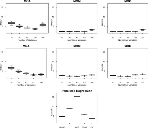
Figure 3. RMSEP for several model averaging (MA) frameworks each with five different numbers of predictors in high-correlation simulated data (Corr: 0.95). There are six MA frameworks: ROA, ROM, ROC, RRA, RRM and RRC. The first letter (‘R’) refers to random partition to construct the candidate models, the second letter corresponds to the candidate model parameter estimation (‘O’ for OLS, and ‘R’ for RR), and the third letter corresponds to the weights (‘A’ for AIC, ‘M’ for Mallows' $C_p$, and ‘C’ for CV). Figures for RMSEP of MA based on marginal correlation model construction are presented in Figure 2. Figures for other correlation structures are presented in the Supplementary Material.

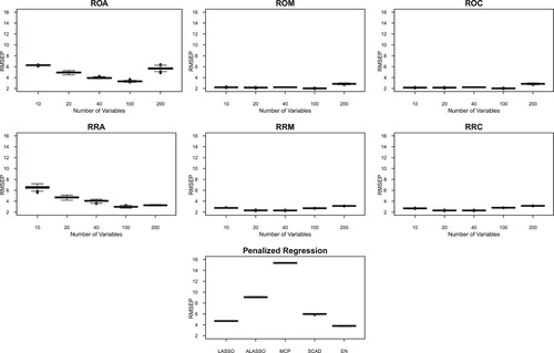
Table 1. Root mean squared error of prediction (RMSEP) from different model averaging (MA) frameworks for different number of variables in the candidate models (v) and in various correlation structures.

		MA framework
Structure of correlation	v	MOA	MRA	MOM	MRM	MOC	MRC	Penalised regression
Low	10	19.240	19.308	16.743	17.325	16.514	17.355	9.193	(LASSO)
	20	17.092	17.244	14.019	15.092	13.279	14.438	10.686	(A-LASSO)
	40	15.960	15.948	11.825	13.331	11.233	12.603	14.961	(MCP)
	100	13.618	13.112	10.025	11.749	9.753	11.193	14.226	(SCAD)
	200	19.186	11.450	12.978	10.724	12.947	10.477	8.088	(Enet)
10 Indep. Block	10	20.913	20.941	18.399	19.053	23.356	24.301	3.728	(LASSO)
	20	19.963	19.870	17.549	18.393	22.291	23.836	4.679	(A-LASSO)
	40	20.168	19.333	17.063	17.905	20.664	22.987	8.222	(MCP)
	100	23.848	18.401	17.140	16.886	18.098	21.204	7.740	(SCAD)
	200	42.854	16.719	27.624	15.223	26.946	18.560	2.904	(Enet)
10 Corr. Block	10	12.236	12.393	4.250	5.022	5.305	6.593	4.009	(LASSO)
	20	9.020	9.503	3.805	4.057	4.025	4.740	7.397	(A-LASSO)
	40	7.994	7.582	3.625	3.668	3.618	3.907	14.927	(MCP)
	100	7.113	5.463	4.527	3.514	4.510	3.578	7.182	(SCAD)
	200	12.071	5.138	8.711	3.707	8.742	3.705	3.954	(Enet)
5 Indep. Block	10	21.093	20.885	16.645	17.205	27.216	28.480	4.628	(LASSO)
	20	20.415	19.687	15.906	16.439	23.892	27.154	6.377	(A-LASSO)
	40	20.424	19.043	15.465	15.978	20.653	24.764	9.647	(MCP)
	100	23.829	18.891	15.287	14.652	16.202	21.389	9.600	(SCAD)
	200	42.402	17.455	26.858	13.141	26.538	19.620	3.198	(Enet)
5 Corr. Block	10	7.516	7.634	2.986	3.435	4.642	5.923	4.181	(LASSO)
	20	5.661	5.601	2.644	2.843	3.108	4.281	7.989	(A-LASSO)
	40	4.619	4.195	2.516	2.554	2.548	3.201	11.160	(MCP)
	100	4.191	2.983	2.595	2.420	2.597	2.416	6.868	(SCAD)
	200	6.482	2.698	4.059	2.542	4.073	2.524	3.884	(Enet)
2 Indep. Block	10	7.137	7.141	2.726	3.315	9.748	11.718	4.969	(LASSO)
	20	5.451	5.309	2.570	2.788	5.940	10.355	7.662	(A-LASSO)
	40	4.612	4.362	2.484	2.582	2.803	8.611	14.010	(MCP)
	100	4.096	3.127	2.543	2.466	2.548	5.972	10.419	(SCAD)
	200	7.991	2.801	4.363	2.423	4.369	2.423	3.883	(Enet)
2 Corr. Block	10	7.354	7.173	2.805	3.262	5.507	7.484	4.351	(LASSO)
	20	5.738	5.482	2.708	2.868	3.949	5.895	9.004	(A-LASSO)
	40	4.463	4.312	2.672	2.750	2.704	4.664	17.298	(MCP)
	100	4.153	3.172	2.677	2.606	2.677	3.269	6.740	(SCAD)
	200	6.231	2.893	3.998	2.679	4.001	2.649	3.961	(Enet)
High (Corr: 0.95)	10	6.714	6.741	2.312	2.845	2.225	2.742	4.699	(LASSO)
	20	5.084	5.025	2.237	2.437	2.224	2.424	9.087	(A-LASSO)
	40	4.150	3.954	2.196	2.380	2.192	2.382	15.367	(MCP)
	100	3.640	3.033	2.173	2.514	2.174	3.074	5.992	(SCAD)
	200	5.711	3.277	3.149	3.023	3.149	3.499	3.807	(Enet)
High (Corr: 0.85)	10	12.058	12.961	4.456	5.068	4.322	4.873	5.536	(LASSO)
	20	9.693	9.548	4.118	4.554	4.098	4.510	11.663	(A-LASSO)
	40	8.023	7.369	3.945	4.322	3.941	4.286	20.328	(MCP)
	100	6.699	5.813	3.764	4.056	3.765	4.048	7.930	(SCAD)
	200	9.896	4.687	5.432	3.845	5.432	3.842	5.235	(Enet)
High (Corr: 0.75)	10	15.279	15.751	5.822	6.927	5.822	6.659	6.467	(LASSO)
	20	12.053	12.444	5.270	6.080	5.270	5.961	11.389	(A-LASSO)
	40	9.707	9.849	4.917	5.648	4.917	5.594	23.358	(MCP)
	100	7.486	6.515	4.801	5.218	4.801	5.193	8.732	(SCAD)
	200	11.863	5.846	6.622	5.058	6.622	5.048	6.090	(Enet)

Notes: There are six MA frameworks: MOA, MOM, MOC, MRA, MRM and MRC. The first letter (‘M’) refers to marginal correlation to construct the candidate models, the second letter corresponds to the candidate model parameter estimation (‘O’ for OLS, and ‘R’ for RR), and the third letter corresponds to the weights (‘A’ for AIC, ‘M’ for Mallows' $C_p$, and ‘C’ for CV). For RMSEP figures where the construction of candidate models is based on random partition, see Table 2. The RMSEP from model selection methods (LASSO, Adaptive LASSO, MCP, SCAD, and Elastic net) are also presented as a comparison.

Table 2. Root mean squared error of prediction (RMSEP) from different model averaging (MA) frameworks for different number of variables in the candidate models (v) and in various correlation structures.

		MA framework
Structure of correlation	v	ROA	RRA	ROM	RRM	ROC	RRC	Penalised regression
Low	10	22.715	21.872	17.105	18.028	16.905	17.805	9.193	(LASSO)
	20	18.378	17.363	13.418	14.333	13.025	14.317	10.686	(A-LASSO)
	40	16.169	16.304	10.759	11.839	10.578	11.833	14.961	(MCP)
	100	14.848	12.393	9.557	10.025	9.453	9.964	14.226	(SCAD)
	200	23.837	10.604	12.975	9.432	12.924	9.378	8.088	(Enet)
10 Indep. Block	10	11.547	11.983	7.178	8.108	11.385	13.202	3.728	(LASSO)
	20	6.223	5.165	2.905	3.168	4.931	4.675	4.679	(A-LASSO)
	40	4.209	4.232	2.273	2.583	2.276	2.598	8.222	(MCP)
	100	3.887	2.804	2.191	2.232	2.190	2.225	7.740	(SCAD)
	200	5.760	2.559	3.112	2.135	3.112	2.131	2.904	(Enet)
10 Corr. Block	10	9.376	9.352	3.079	3.707	3.299	4.119	4.009	(LASSO)
	20	5.796	5.760	2.521	2.741	2.526	2.775	7.397	(A-LASSO)
	40	4.506	4.246	2.367	2.450	2.367	2.450	14.927	(MCP)
	100	3.875	3.028	2.278	2.339	2.278	2.338	7.182	(SCAD)
	200	6.039	2.462	3.206	2.381	3.206	2.391	3.954	(Enet)
5 Indep. Block	10	7.707	8.209	2.900	3.932	6.564	9.245	4.628	(LASSO)
	20	6.215	5.525	2.552	2.673	2.575	2.695	6.377	(A-LASSO)
	40	4.726	4.519	2.394	2.440	2.392	2.429	9.647	(MCP)
	100	3.753	3.238	2.375	2.367	2.375	2.359	9.600	(SCAD)
	200	6.304	2.753	3.461	2.321	3.461	2.316	3.198	(Enet)
5 Corr. Block	10	7.268	7.275	2.522	3.034	2.655	3.409	4.181	(LASSO)
	20	5.434	5.264	2.290	2.460	2.286	2.468	7.989	(A-LASSO)
	40	4.257	3.988	2.203	2.279	2.202	2.278	11.160	(MCP)
	100	3.744	2.411	2.185	2.210	2.185	2.215	6.868	(SCAD)
	200	5.955	2.570	3.147	2.424	3.147	2.456	3.884	(Enet)
2 Indep. Block	10	6.916	6.830	2.475	2.944	2.435	2.974	4.969	(LASSO)
	20	5.211	5.017	2.321	2.442	2.320	2.440	7.662	(A-LASSO)
	40	4.222	3.883	2.234	2.307	2.234	2.304	14.010	(MCP)
	100	3.762	2.971	2.233	2.219	2.232	2.217	10.419	(SCAD)
	200	6.012	2.464	3.216	2.181	3.216	2.179	3.883	(Enet)
2 Corr. Block	10	7.019	6.871	2.442	2.848	2.370	2.832	4.351	(LASSO)
	20	5.328	5.242	2.323	2.454	2.315	2.447	9.004	(A-LASSO)
	40	4.325	3.927	2.257	2.333	2.255	2.331	17.298	(MCP)
	100	3.829	2.425	2.258	2.286	2.258	2.293	6.740	(SCAD)
	200	6.142	2.673	3.294	2.534	3.294	2.572	3.961	(Enet)
High (Corr: 0.95)	10	6.265	6.524	2.214	2.770	2.154	2.690	4.699	(LASSO)
	20	4.920	4.700	2.164	2.328	2.151	2.306	9.087	(A-LASSO)
	40	3.959	4.046	2.232	2.305	2.231	2.305	15.367	(MCP)
	100	3.326	2.987	2.019	2.716	2.019	2.808	5.992	(SCAD)
	200	5.669	3.265	2.853	3.132	2.853	3.162	3.807	(Enet)
High (Corr: 0.85)	10	11.533	11.415	4.248	4.706	4.184	4.658	5.536	(LASSO)
	20	8.929	8.641	3.928	4.197	3.927	4.190	11.663	(A-LASSO)
	40	7.152	6.726	3.796	3.951	3.795	3.943	20.328	(MCP)
	100	6.404	5.074	3.763	3.770	3.762	3.764	7.930	(SCAD)
	200	10.001	4.334	5.395	3.707	5.395	3.702	5.235	(Enet)
High (Corr: 0.75)	10	14.834	14.752	5.565	6.215	5.524	6.181	6.467	(LASSO)
	20	11.348	10.983	4.968	5.436	4.962	5.425	11.389	(A-LASSO)
	40	9.168	8.563	4.756	5.042	4.753	5.032	23.358	(MCP)
	100	8.190	6.466	4.727	4.789	4.726	4.777	8.732	(SCAD)
	200	12.837	5.563	6.874	4.704	6.873	4.694	6.090	(Enet)

Notes: There are six MA frameworks: ROA, ROM, ROC, RRA, RRM and RRC. The first letter (‘R’) refers to random partition method to construct the candidate models, the second letter corresponds to the candidate model parameter estimation (‘O’ for OLS, and ‘R’ for RR), and the third letter corresponds to the weights (‘A’ for AIC, ‘M’ for Mallows' $C_p$, and ‘C’ for CV). For RMSEP figures where the construction of candidate models is based on marginal correlation, see Table 1. The RMSEP from model selection methods (LASSO, Adaptive LASSO, MCP, SCAD, and Elastic net) are also presented as a comparison.

In Table 1, there are a few situations in which MA has higher RMSEP than model selection methods. This is true in the case of low correlation, 10 independent block correlation, and 5 independent block correlation. Other than those, MA manages to obtain lower RMSEP than the model selection methods. In Table 2, MA manages to obtain a lower RMSEP than the model selection methods in all situations, except the low-correlation setting. This is encouraging, considering that the simulation settings considered are relatively challenging with different correlation structures.

In terms of the number of predictors in the candidate models, Tables 1 and 2 indicate that the RMSEP decreases as the number of predictors in the candidate models increases. However, when the model parameters are estimated using OLS, the RMSEP tends to increase again when the number of predictors is 200 in the candidate models. This indication is generally not seen when we consider ridge regression estimates. This is reasonable because when the number of predictors in the candidate models increases to n, then the OLS estimation becomes unstable and the ridge regression estimate is known to be able to deal with this problem. Furthermore, having 100 (n/3) and 200 (2n/3) predictors in the candidate models tends to give optimal predictions when using ridge regression estimates. When the OLS estimation is considered, the general tendency is to consider having 100 predictors in the candidate models for a good prediction. These results indicate that the estimation of model parameters interacts with the number of predictors in the candidate models for an optimal prediction in MA.

In terms of methods to construct candidate models, we find from Tables 1 and 2 that both marginal correlation and random partition methods have comparable performance, except in the case of block correlation with 5 and 10 independent blocks. In these two cases, the tables suggest that random partition is preferable to construct candidate models. In the context of high correlation between variables such as the case in the calibration of NIR instruments, the tables show that the RMSEP is quite similar and they both give lower RMSEP than that from model selection methods. Lastly, in terms of methods to calculate weights for candidate models in MA, Tables 1 and 2 show that the weights based on Mallows' $C_p$ and cross-validation criteria give lower RMSEP than those based on AIC, across different correlation structures of the simulated data.

4.2. NIR calibration data

The results of the MA on real NIR calibration data are presented in Table 3. The table shows the RMSEP on the two NIR datasets across different numbers of predictors in the candidate models (v). The numbers of predictors tested in the real data are n/4, n/3, and n/2. This is based on a ratio over n that gives the optimal RMSEP in the simulation study of approximately n/3. The table indicates that in the Corn (mp5) data, the MA gives lower RMSEP than the model selection methods in all outcome variables. However, in the Corn (mp6) data, MA only gives lower RMSEP when the outcome variable is oil content. For the other outcome variables, MA gives a higher RMSEP than the model selection methods.

Table 3. RMSEP's of the calibration models in the NIR datasets under the different frameworks of model averaging (MA) in comparison with model selection methods (LASSO, Adaptive LASSO, MCP, SCAD, and Elastic Net).

Data	Response	v	MA framework						Penalised
Corn (mp5)	Moisture	20	0.510	0.456	0.472	0.319	0.374	0.302	0.341	(LASSO)
		28	0.512	0.485	0.517	0.318	0.379	0.377	0.588	(A-LASSO)
		35	0.528	0.523	0.510	0.317	0.377	0.402	0.401	(MCP)
									0.470	(SCAD)
									0.401	(Enet)
	Oil	20	0.218	0.209	0.216	0.172	0.183	0.180	0.184	(LASSO)
		28	0.233	0.215	0.223	0.172	0.176	0.178	0.451	(A-LASSO)
		35	0.242	0.234	0.254	0.172	0.177	0.176	0.179	(MCP)
									0.436	(SCAD)
									0.196	(Enet)
	Protein	20	0.636	0.576	0.673	0.469	0.496	0.489	0.536	(LASSO)
		28	0.669	0.642	0.653	0.491	0.500	0.499	0.805	(A-LASSO)
		35	0.705	0.687	0.674	0.490	0.494	0.494	0.497	(MCP)
									1.151	(SCAD)
									0.568	(Enet)
	Starch	20	1.021	1.036	0.986	0.490	0.834	0.840	0.832	(LASSO)
		28	1.031	0.988	1.026	0.836	0.869	0.833	0.644	(A-LASSO)
		35	1.088	1.053	1.073	0.836	0.906	0.804	1.006	(MCP)
									0.790	(SCAD)
									0.912	(Enet)
Corn (mp6)	Moisture	20	0.499	0.451	0.446	0.318	0.378	0.383	0.248	(LASSO)
		28	0.518	0.475	0.478	0.317	0.382	0.379	0.239	(A-LASSO)
		35	0.529	0.518	0.525	0.381	0.301	0.379	0.275	(MCP)
									0.316	(SCAD)
									0.379	(Enet)
	Oil	20	0.222	0.210	0.196	0.176	0.178	0.179	0.240	(LASSO)
		28	0.223	0.212	0.218	0.177	0.208	0.178	0.283	(A-LASSO)
		35	0.243	0.234	0.235	0.177	0.179	0.174	0.182	(MCP)
									0.235	(SCAD)
									0.184	(Enet)
	Protein	20	0.645	0.593	0.683	0.497	0.508	0.503	0.244	(LASSO)
		28	0.678	0.637	0.608	0.493	0.497	0.500	0.531	(A-LASSO)
		35	0.704	0.679	0.674	0.494	0.484	0.495	0.548	(MCP)
									0.360	(SCAD)
									0.496	(Enet)
	Starch	20	1.088	1.045	0.894	0.835	0.852	0.835	0.891	(LASSO)
		28	1.018	0.974	0.984	0.832	0.822	0.832	0.848	(A-LASSO)
		35	1.072	1.051	1.046	0.834	0.887	0.836	0.832	(MCP)
									0.964	(SCAD)
									0.589	(Enet)

Notes: There are six MA frameworks: MOA, MOM, MOC, MRA, MRM and MRC. The first letter (‘M’) refers to marginal correlation to construct the candidate models, the second letter corresponds to the candidate model parameter estimation (‘O’ for OLS, and ‘R’ for RR), and the third letter corresponds to the weights (‘A’ for AIC, ‘M’ for Mallows' $C_p$, and ‘C’ for CV).

Table 3 indicates that MA frameworks with ridge estimation produce less RMSEP than those with OLS estimates. This reflects the situation that we observed previously in the simulation study. It is also interesting to note that the application of MA on real datasets indicates that the choice of weights is less crucial. The lowest RMSEP within each outcome variable in the MA framework can be obtained by weights based on AIC, Mallows' $C_p$, and cross validation. Although, it is important to note that all these minimums are achieved only when the parameters are estimated using ridge regression.

5. Discussion and concluding remarks

We have investigated the impact of different numbers of predictors, parameter estimation methods, and weighting schemes on prediction within the MA frameworks. Our investigation indicates that increasing the number of predictors in the candidate model is expected to better the prediction performance in general. However, this is consistent when we consider the ridge regression to estimate the candidate models' parameters. When we consider OLS estimates, the prediction starts to be negatively affected when the number of predictors is getting closer to the number of observations. This is a main result that is important to note as all known studies in MA, to our knowledge, have consistently utilised only the OLS estimation method. With the ridge estimates, our simulation study has indicated a stable performance in prediction.

The results of the simulation study also indicated that the Mallows' $C_p$ and CV weights are more beneficial for prediction compared to the AIC weights. Overall, the Mallows' $C_p$ is generally preferred, as this is shown to be consistent across different correlation structures of simulated data. The advantage of MA compared to the model selection methods (LASSO, Adaptive LASSO, MCP, SCAD, and Elastic Net) is visible in all correlation structures within the simulated data, except in the case of lower correlation setting. In the context of ten and five independent block correlation, MA still has the advantage compared to the model selection methods when we construct the candidate models using random partition, but not when using marginal correlation. In the different settings of high-correlation simulated data, such as the case in the calibration of NIR instruments, we find that the MA is generally better than the model selection methods. These simulation results are important to guide researchers on whether to consider MA or model selection approach in prediction. In particular, many areas such as molecular biology, medicine, and social sciences usually deal with clusters of variables in their data. So, a careful check on the correlation structure of data is necessary when considering which approach to use.

The principles that we learned from the simulation study, to much extent, are also seen in the real data application. The ridge model averaging is shown to be generally superior compared to the more common OLS MA. The ridge MA also produces lower RMSEP than the model selection methods in the Corn (mp5) data. In the Corn (mp6) data, the ridge MA only produces lower RMSEP than the model selection methods when the outcome variable is oil. This suggests that, in the context of calibration of NIR instruments with correlated high-dimensional data, we still consider the MA approach to be a preferred alternative.

For the number of predictors in the candidate models v, we find from the simulation study that n/3 is generally preferable to achieve an optimal prediction for both OLS and ridge regression estimation in the MA framework. This should be considered as a rule of thumb rather than a prescription. In the real data application where v is set to be n/4, n/3 and n/2, MA managed to achieve better RMSEP than the model selection methods in the majority of outcome variables.

As an idea for extension, we can consider e.g. a model selection approach for each candidate model within the MA framework. This is currently our active research and is beyond the scope of this manuscript. There are some complications to consider in this ‘hybrid’ approach. However, we believe that this research is still necessary to arrive at a MA framework that potentially improves further its prediction ability in data with different correlation structures. Lastly, it is important to note that in the calibration of NIR instruments, it is common to have multivariate outcomes such as in our datasets. In this case, we can consider the MA framework in a multivariate response setting, although we did not consider that in this study. Overall, we feel that MA provides an opportunity for better prediction in the calibration problem compared to model selection methods, despite some remaining issues for future works.

Acknowledgments

The first author (DTS) would like to thank the School of Mathematics, University of Leeds, UK, for hosting her research visit.

Additional information

Funding

The first author (DTS) was supported by the 2016 PKPI scholarship provided by the Ministry of Research, Technology and Higher Education of Indonesia.

References

- Eigenvector Research, Inc. NIR of Corn Samples for Standardization Benchmarking, 2021. Available at https://www.eigenvector.com/data/Corn/, accessed 2 May 2021.
- T. Ando and K.C. Li, A model-averaging approach for high dimensional regression, J. Am. Stat. Assoc. 109 (2014), pp. 254–265.
- S.T. Buckland, K.P. Burnham, and N.H. Augustin, Model selection: an integral part of inferences, Biometrics 53 (1997), pp. 603–618.
- P. Buhlmann and S. Van de Geer, Statistics for High-Dimensional Data, Spinger-Verlag, Berlin, 2011.
- K.P. Burnham and D. Anderson, Model Selection and Multimodel Inference: A Practical Information-Theoritic Approach, Spinger-Verlag, Berlin, 2002.
- G. Claeskens and N. Hjort, Model Selection and Model Averaging, Cambridge University, New York, 2008.
- J. Fan and R. Li, Variable selection via nonconcave penalized likelihood and its oracle properties, J. Am. Stat. Assosiation 96 (2001), pp. 1348–1360.
- A. Gusnanto, Y. Pawitan, J. Huang, and B. Lane, Variable selection in random calibration of near infrared instruments: ridge regression and partial least squares regression settings, J. Chemom. 17 (2003), pp. 174–185.
- B.E. Hansen, Least squares model averaging, Econometrica 75 (2007), pp. 1175–1189.
- B.E. Hansen and J. Racine, Jackknife model averaging, J. Econom. 167 (2012), pp. 34–38.
- A.E. Hoerl and R.W. Kennard, Ridge regression: biased estimation for nonorthogonal problems, Technometrics 12 (1970), pp. 55–67.
- Q. Liu, R. Okui, and A. Yoshimura, Generalized Least Squares Model Averaging, SSRN Working Paper, Kyoto University, Kyoto, 2014.
- J. Magnus, O.R. Powell, and P. Prufer, A comparison of two model averaging techniques with application to growth empiric, J. Econom. 154 (2010), pp. 139–153.
- Y. Pawitan, In All Likelihood: Statistical Modelling and Inference Using Likelihood, Oxford University Press, New York, 2013.
- A. Raftery, D. Madigan, and J. Hoeting, Bayesian model averaging for linear regression models, J. Am. Stat. Assoc. 92 (1997), pp. 179–191.
- D.T. Salaki, A. Kurnia, A. Gusnanto, I.W. Mangku, and B. Sartono, Model averaging in calibration model, IJSRSET 4 (2018), pp. 189–195.
- R. Tibhsirani, Regression shrinkage and selection via the lasso, J. R. Stat. Soc. Ser. B 58 (1996), pp. 267–288.
- R. Tibhsirani, The lasso problem and uniqueness, Electron. J. Stat. 7 (2013), pp. 1456–1490.
- C.H.. Zhang, Nearly unbiased variable selection under minimax concave penalty, Ann. Stat. 38 (2010), pp. 894–942.
- S. Zhao, J. Zhou, and H. Li, Model averaging with high-dimensional dependent data, Econ. Lett. 146 (2016), pp. 68–71.
- H. Zou, The adaptive lasso and its oracle properties, J. Am. Stat. Assoc. 101 (2006), pp. 1418–1429.
- H. Zou and T. Hastie, Regularization and variable selection via the elastic net, J. R. Stat. Soc. Ser. B67 (2005), pp. 301–320.