Artificial neural network study of the electrical conductivity of mould flux

Abstract

The electrical conductivity of mould flux with chemical constitution of CaO-SiO₂-Al₂O₃-NaO-K₂O-MgO-CaF₂-Cr₂O₃-FeO-MnO has been investigated. The assessed database contains one unitary, five binary, nine ternary, four quaternary, two quinary, two senary and one octonary subsystems. Each constitutional component is in connection to another via some direct or indirect links. A multilayer artificial neural network method was developed and implemented in the database. The work provides a method to calculate the relationships between the composition, temperature and electrical property of the mould flux within the defined parameter ranges. The results have been validated against those experimental data that are not included in the training of the neural networks.

KEYWORDS:

• Electrical conductivity
• mould flux
• multilayer neural network
• continuous casting

Introduction

Many steelmaking companies are using a mould flux with chemical constitution of CaO-SiO₂-Al₂O₃-NaO-K₂O-MgO-CaF₂-Cr₂O₃-FeO-MnO to cast stainless steels in continuous casting mould. The mould slag contains high concentration of fluorine to reduce viscosity and solidification temperature [1]. Cr₂O₃-FeO-MnO can either pre-exist in mould powder or enter to liquid slag from oxidation of alloying elements in liquid stainless steel at casting mould and tundish [2]. The electrical conductivity of this system has never been assessed systematically although the data for its subsystem are notably rich.

The primary driving force to study the electrical properties of mould powder is for electroslag remelting processing [3,4]. This has, therefore, attracted considerable experimental measurement activities [3–6], theoretical modelling [7,8] and data assessment [9] for several subsystems. The recent environment regulation on carbon neutral steelmaking promotes the electrification of continuous casting. Electric field affects materials segregation [10], viscosity [11], distribution of oxide inclusions [12] and surface roughness in the cast mould [13]. This demands an analytical expression to represent the relationship between the chemical constitution, temperature and electrical conductivity of the system. The aim of the present work was to provide a mean to calculate the constitution and temperature-dependent electrical conductivity of the mould flux materials.

This work uses artificial neural network to approach the target. The method relies on available data to extrapolate values in the unknown parameters’ range [14]. Ideally, a relationship between the electrical conductivity, constitution and temperature should be derived from micro-mechanisms [15]. The previous theoretical modelling for the electrical conductivity of mould slag has been based largely on an assumption that electrical conduction is carried out by the moving ionised atoms. Obviously, viscosity affects the mobility of ionised atoms and hence plays an important role in electrical conduction. The basicity of mould slag affects the amount and length of silicate chains. This lays a foundation for the optical basicity model to calculate the electrical conductivity of mould slag [7]. On the other side, the interactions between constitutional components influence the mobility of atoms. This forms a basis to use particle interaction to calculate electrical conductivity [8]. For the oxides which can conduct electricity by electronic means, such as FeO, the above-mentioned theoretical models stray away [2]. The data-based artificial neural network has proved to be an effective solution to provide alternative solution [9].

The artificial neural network is different from data fitting such as the least square method. The former prevents overfitting but the latter seeks best fitting to data. The recent development of artificial intelligent learning enables the method to reduce its dimension according to the conservative laws that are hidden in the data [16,17]. Artificial neural network has potential to indicate some physics natures buried in the big data. This work intends to provide a method to calculate the constitution and temperature-dependent electrical conductivity of the mould flux.

Artificial neural network

A supervised multilayer artificial neural network with back propagation learning algorithm has been coded for the present purpose. The network has an input layer containing 11 units to record the constitutional compositions and temperature. The output layer has 1 unit to provide the computational result for electrical conductivity. There are T-1 hidden layers each containing numerous units. The architecture of 2-layer network is illustrated schematically in Figure 1, where the hidden layer has n-units. The mapping function for 2-layer neural network in the present work is defined as (1.1) $\begin{array}{rl}{x}_j& ={\sum }_{i=1}^{10}{\omega }_{j,i}^{(1)}{c}_i+{\omega }_{j,11}^{(1)}T+b_j^{(1)}\end{array}$(1.1) (1.2) $\begin{array}{rl}{u}_j& =1/(1+e^{-x_j})\end{array}$(1.2) (1.3) $\begin{array}{rl}y& ={\sum }_{j=1}^n{\omega }_{1,j}^{(2)}{u}_j+b_1^{(2)}\end{array}$(1.3) (1.4) $\begin{array}{rl}\sigma & =1/(1+e^{-y})\end{array}$(1.4)

Figure 1. Schematic diagram illustrates 2-layer neural network.

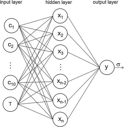
The mapping function for >2 layers neural network can be manipulated in the same way. A code package to calculate up to 4-layer neural network has been developed by the author. ${\omega }_{j,i}^{(k)}$ is the weight factor between j^th unit in k^th layer and i^th unit in (k−1)^th layer, where 0^th layer is the input layer. $b_j^{(k)}$ is the bias for j^th unit in k^th layer. $x_j$ is the activation of j^th unit in 1^st layer $u_j$ is its activation function. $y$ is the activation of output layer. The electrical conductivity $\sigma$ is the activation function of $y$.

The activation functions in Equations (1.2) and (1.4) are nonlinear and with output values between 0 and 1. Many other neural network models choose other functions such as $f(x)=\text{tanh}(x)$ [14], which has value between −1 and 1, or Gaussian distribution [16]. It is important to normalise the data according to the format of activation functions. In the present model, all the electrical conductivity data are normalised to a value between 0 and 1. The numerical results are denormalised to get the true value.

Following the standard method in neural network calculation [18], the total difference is defined as (2) $\begin{array}{r}{E}_D=\frac{1}{m}{\sum }_{l=0}^m{({\sigma }_c^{(l)}-{\sigma }_e^{(l)})}^2\end{array}$(2) where m is the total number of sets of training data. ${\sigma }_e^{(l)}$ and ${\sigma }_c^{(l)}$ are the l^th training value and calculated value, respectively. To prevent neural network optimisation from overfitting the noise in training data, a regularisation is defined to minimise the total value of weight factor square as $E_W={\sum }_{i,j,k}{(w_{j,i}^{(k)})}^2$. The overall target function is defined as [18] (3) $\begin{array}{r}E=\frac{1}{2}\beta E_D+\frac{1}{2}\alpha E_W\end{array}$(3) where β and α are coefficients. Their ratio reflects a balance between accuracy and simplicity. The intelligent learning is to perform a gradient descent minimisation of the total difference via [19] (4) $\begin{array}{r}\mathrm{\Delta }{w}_{j,i}^{(k)}=-\eta \mathrm{\partial }E/\mathrm{\partial }{w}_{j,i}^{(k)}\end{array}$(4) where $\eta$ is the learning rate. Equation (4) defines one of the learning methods that always works but unnecessarily the most effective method. In the following section, other learning methods will be used and compared with Equation (4). The analytical expression for each weight factor and bias can be obtained by back propagation of the partial difference of target function according to Equation (4).

Data assessment

The composition in the database is defined to be atomic percentage. The weight percentage data from literature has been converted according to their molar weight [3,5,6,21]. Renormalisation has been performed for those data that the original total composition does not come to 100% [22]. This is not rare in steel company become the initial constitutions of C and CO₂ in mould powder are not counted in liquid slag. However, some data in literature has a total composition in excess of 100%. Those data are ignored entirely. For the data contain tiny fraction (3.00 wt-%) of NaO and K₂O but without detailed information about their ratio [21]. An assumption of 50:50 is applied. This assumption does not affect the specification of the individual contribution from NaO and K₂O to the electrical conductivity because a significant amount of NaO and K₂O data from other literature has been applied to justify the assumption [23,24]. For the data that have been assessed previously [8], the assessed data instead of large amount of raw experimental data has been adopted to minimise noise. Some data are reported as scattered points in plotted figure. To get the values from the plotted figure with high accuracy, a java-based code package has been developed by the author to convert the figure to data. Some figures have been plotted artificially with scales in coordinates not proportional [22]. Only those data with clear indication of their values have been adopted. For the plotted continuous curves, only those points accompanied with experimental values are adopted. After the critical assessment, a database contains 752 sets of data with one unitary, five binary, nine ternary, four quaternary, two quinary, two senary and one octonary subsystems has been built up. The detailed subsystems are listed in Table 1. The parameter ranges are shown in Table 2. The unit of temperature is Kelvin. The unit of electrical conductivity is Ω⁻¹·cm⁻¹.

Table 1. The subsystems in the electrical conductivity database.

No. Components	System	Reference
1	CaF2	[3,6]
2	CaO + SiO2	[8,23]
2	CaO + Al2O3	[4,8]
2	CaO + CaF2	[3,4,8]
2	Al2O3 + CaF2	[3,4]
2	MgO + CaF2	[4]
3	CaO + SiO2 + Al2O3	[5,7]
3	CaO + SiO2 + NaO	[23,24]
3	CaO + SiO2 + K2O	[23]
3	CaO + SiO2 + CaF2	[6]
3	CaO + Al2O3 + CaF2	[3]
3	SiO2 + Al2O3 + NaO	[24]
3	SiO2 + NaO + FeO	[24]
3	SiO2 + NaO + MgO	[24]
3	SiO2 + NaO + MnO	[24]
4	CaO + SiO2 + Al2O3 + NaO	[24]
4	CaO + SiO2 + NaO + K2O	[23]
4	CaO + SiO2 + Al2O3 + K2O	[23]
4	CaO + SiO2 + Al2O3 + MgO	[23]
5	CaO + SiO2 + Al2O3 + NaO + K2O	[4,5,7]
5	CaO + SiO2 + Al2O3 + CaF2 + FeO	[23]
6	CaO + SiO2 + Al2O3 + MgO + CaF2 + FeO	[22]
6	CaO + SiO2 + Al2O3 + MgO + FeO + MnO	[4,22]
8	CaO + SiO2 + Al2O3 + NaO + K2O + MgO + CaF2 + Cr2O3	[21]

Table 2. The range of parameters’ values in the database.

					(at.-%)						(K)
Value	CaO	SiO2	Al2O3	NaO	K2O	MgO	CaF2	Cr2O3	FeO	MnO	T
Min	0	0	0	0	0	0	0	0	0	0	471
Max	72.24	60.81	43.24	29.21	6.00	20.00	100.00	0.523	34.80	20.00	2039

Neural network computation and results

The activation functions, as illustrated in Equations (1.2) and (1.4), have an output value between 0 and 1 for the activation between -∞ and +∞. However, $\sigma =0.006693$ at $y=-5$ and $\sigma =0.993307$ at $y=5$, which indicate an extremely slow approximation to either 0 or 1. Based on this consideration, the training data for electrical conductivity is not normalised by the true minimum and maximum values in the database but multiplied by 0.7 to the minimum value and 1.3 to the maximum value. The input parameters for composition and temperature are all normalised to a value between 0 and 1 to ensure every input parameter has the same weight of contribution. The denormalisation and normalisation procedure followed the following equations (5.1) $\begin{array}{rl}\tilde{\sigma }& =\frac{\sigma -0.7{\sigma }^{min}}{1.3{\sigma }^{max}-0.7{\sigma }^{min}}\end{array}$(5.1) (5.2) $\begin{array}{rl}{\tilde{c}}_i& =\frac{c_i-c_i^{min}}{c_i^{max}-c_i^{min}}\end{array}$(5.2) where $\tilde{\sigma }$ and ${\tilde{c}}_i$ are the normalised electrical conductivity and composition for $i<11$ and temperature when $i=11$. The initial values for all the weight factors and biases are assigned to a random float value between −5 and 5. A high-quality random number generator was coded according to a probability theory developed by Marsaglia et al. [25].

In neural network calculation, it has been noted that the artificial learning by means of Equation (4) in every time iteration does not help to find the weight factors and biases to achieve minimum total differences between the target values and calculated value. The weight factors soon adjust their values to minimise the overall target function ($E$) rather than the total difference ($E_D$). To overcome this problem, the regularisation term ($E_W$) is not included in each time iteration but replaced at the final step assessment. It is also found that the convergence rate is almost doubled by the following artificial learning mechanism, which agrees with the suggestion from Rumelhart et al. [19] (6) $\begin{array}{r}\mathrm{\Delta }{w}_{j,i}^{(k)}(t+1)=-\eta \mathrm{\partial }E/\mathrm{\partial }{w}_{j,i}^{(k)}+\delta \mathrm{\Delta }{w}_{j,i}^{(k)}(t)\end{array}$(6) where δ is a coefficient. 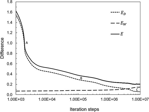For the 2-layer neural network calculation with $n=16$ and $\alpha =\beta =\eta =\delta =0.5$, the evolution of total difference, regularisation term and target function vs iteration steps are demonstrated in Figure 2. It shows that that total difference drops sharply in the early stage (labelled by A), followed by slow drops (labelled by B) until a flat stage (labelled by C) to fluctuate around a minimum value. However, the regularisation term was increased slowly but monotonically until stage C. This is due to the early mentioned decision of not to include the minimisation of regularisation term in the time iteration. The target function has been reduced monotonically until the flat stage.

Figure 2. The evolution of total difference ($E_D$), regularisation term ($E_W$) and target function ($E$) vs. iteration steps for 2-layer neural network with hidden layer containing 16 units.

To determine the optimum number of units in the hidden layer in 2-layer neural network calculation, one has calculated the change of differences until 1.6 × 10⁷ iteration steps for various number of units. The results are plotted in Figure 3. Although $E_D$ decreases when the number of units increases, $E_W$ demonstrates some optimised values. $E_W$ increases sharply when the number of units is away from the optimised one. The target function, $E$, reveals an optimised value for the number of units in the hidden layer of the 2-layer neural network. Based on the results, $n=16$ is chosen. It is worth mentioning that the local minimum at $n=16$ for the curve of $E_D$ is out of expectation. To double check whether it is a numerical coincidence, the code and parameters were run at three different workstations but the results were very similar, given the fact that the initialisation of weight factors involves a random number generator which should be different at different computers. The smallest $E_D$ appeared at 9,012,000^th iteration step. The values for the weight factors and biases at this optimised condition are listed in Table 3. These values can be used to calculate the electrical conductivity of the system at any composition and temperature in the parameters’ range.

Figure 3. The evolution of total difference ($E_D$), regulation term ($E_W$) and target function ($E$) vs. number of units in hidden layer after 1.6 × 10⁷ iteration steps.

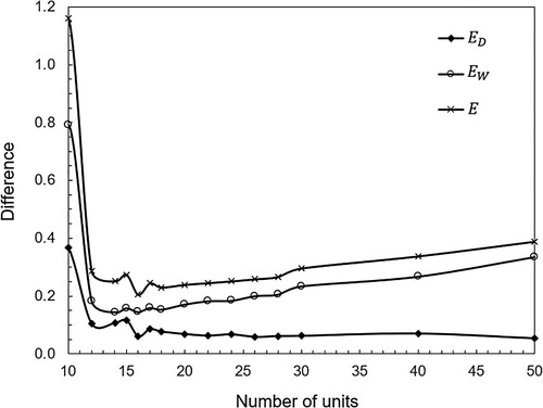
Table 3. The optimised weight factors and biases obtained by artificial neural network calculations.

$\mathit{i}$	1	2	3	4	5	6	7	8	9	10	11	12	13	14	15	16
${\mathit{\omega }}_{1,\mathit{i}}^{(1)}$	−3.522	−1.679	4.007	−1.131	−4.703	1.314	−3.504	−1.977	−1.589	−2.611	−3.141
${\mathit{\omega }}_{2,\mathit{i}}^{(1)}$	2.222	−0.300	−1.014	2.707	5.379	−4.533	3.134	5.043	−6.042	1.987	6.161
${\mathit{\omega }}_{3,\mathit{i}}^{(1)}$	2.046	−4.629	−0.695	−6.015	3.567	−0.802	0.999	9.960	−0.642	−4.569	0.939
${\mathit{\omega }}_{4,\mathit{i}}^{(1)}$	0.932	2.293	0.716	4.157	0.552	−3.415	−1.466	−6.693	−3.632	0.258	−6.973
${\mathit{\omega }}_{5,\mathit{i}}^{(1)}$	−2.666	10.377	−0.491	−0.494	−4.455	−5.990	1.666	−1.483	−4.617	−2.839	−0.185
${\mathit{\omega }}_{6,\mathit{i}}^{(1)}$	2.605	−1.698	−2.027	−3.533	3.922	3.881	−5.338	0.311	−0.906	−4.354	−0.171
${\mathit{\omega }}_{7,\mathit{i}}^{(1)}$	4.777	2.718	−4.250	0.815	7.090	5.123	−3.763	6.540	−4.007	−0.648	3.776
${\mathit{\omega }}_{8,\mathit{i}}^{(1)}$	−7.403	2.192	1.479	3.087	−5.408	0.885	−1.703	−6.276	3.248	−0.600	−6.350
${\mathit{\omega }}_{9,\mathit{i}}^{(1)}$	−3.031	−0.087	5.793	−0.693	−1.810	−3.520	5.388	−0.979	−3.414	1.390	−3.816
${\mathit{\omega }}_{10,\mathit{i}}^{(1)}$	−5.049	3.333	−2.414	−3.978	0.912	1.814	4.518	0.182	2.548	2.945	−1.225
${\mathit{\omega }}_{11,\mathit{i}}^{(1)}$	−0.267	−1.132	−3.102	3.209	−0.603	−7.334	−3.738	0.064	5.103	2.639	5.318
${\mathit{\omega }}_{12,\mathit{i}}^{(1)}$	0.376	−2.656	−0.931	1.841	−0.312	3.175	−0.627	−6.724	−1.493	−0.382	−2.201
${\mathit{\omega }}_{13,\mathit{i}}^{(1)}$	1.860	−8.368	−5.901	6.286	−1.250	0.786	2.651	0.438	2.259	0.032	6.445
${\mathit{\omega }}_{14,\mathit{i}}^{(1)}$	−2.727	5.957	3.358	2.482	2.415	7.337	−1.195	−8.983	2.609	−0.273	−3.009
${\mathit{\omega }}_{15,\mathit{i}}^{(1)}$	−0.862	1.249	−5.116	5.106	−2.449	0.498	−3.733	−3.322	4.180	0.328	−1.869
${\mathit{\omega }}_{16,\mathit{i}}^{(1)}$	1.730	0.858	−0.612	−2.560	−0.201	−1.836	1.620	−6.329	−2.162	−1.012	1.505
${\mathit{\omega }}_{1,\mathit{i}}^{(2)}$	−0.173	9.125	0.146	3.450	−8.575	2.630	6.701	4.235	−0.306	1.920	−4.530	−10.039	8.650	−9.208	−1.216	1.997
${\mathit{b}}_{{\mathit{i}}^{(1)}}$	1.172	0.645	0.321	−2.985	4.332	−5.004	2.231	6.241	6.158	4.916	−2.561	3.300	0.997	5.489	−3.383	3.552
${\mathit{b}}_{{\mathit{i}}^{(2)}}$	−6.009

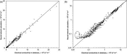
The optimised weight factors and bias values have been implemented to calculate the electrical conductivity for 752 sets of compositions and temperature. The results are plotted in Figure 4 and compared with the values in the database. Figure 4(a) shows the comparison at linear scale coordinates. The 45° line indicates the perfect agreement between the artificial neural network computational results and the value in database, where majority data are from experimental measurement and the rest from assessment based on experimental values. The figure shows good agreement. Owing to the wide range distribution of the electrical conductivity values from 0.016 to 23.771, which across three orders of magnitude, the comparison in logarithmic scale is shown in Figure 4(b). The data shows some almost evenly distribution around the 45° line, majority with absolute error below 5%. The largest absolute discrepancy appears in the lowest electrical conductivity end, as is circled in Figure 4(b). Those data are found all belong to CaO-SiO₂-Al₂O₃ subsystem at a temperature either in 1623 K or 1673 K, and was reported in one paper.

Figure 4. The electrical conductivity from numerical results by artificial neural network calculation vs. the value in the database: (a) in linear scale plotting, and (b) in logarithmic scale plotting.

To validate the artificial neural network calculations, the optimised weight factors and bias values have been implemented to calculate two binary systems CaF₂-Al₂O₃ and Cao-CaF2 at different temperature. The results have been compared with the experimental results reported in various literature [6,26,27]. Figure 5 presents the results for (a) CaF₂-Al₂O₃ at 1773K, (b) CaF₂-Al₂O₃ at 1973K, (c) Cao-CaF2 at 1773K and (d) Cao-CaF2 at 1873K. These experimental data are not in database during the training of neural network. Figure 5 shows that the electrical conductivity obtained in the neural network calculations are within the fluctuation of various experimental measurements. It proves that the artificial neural network prediction for the electrical conductivity can be used to predict the change of electrical conductivity at various subsystems in different compositions and temperatures.

Figure 5. Validation of neural network calculation by experimental data reported in literature [6,26,27]. (a) CaF₂-Al₂O₃ at 1773K, (b) CaF₂-Al₂O₃ at 1973K, (c) Cao-CaF2 at 1773K, and (d) Cao-CaF2 at 1873K.

The artificial neural network and machine learning have many potential applications in steel metallurgy [28]. In the future, more works will be done to include other components to the system, such as NiO, TiO₂, MgF₂, BaF₂, BaO, ZrO, CaS. The availability of the new experimental measurement method for electrical conductivity enables to get more accurate data in other systems [29], which will help to build up database for training and validation of the neural networks. The future work can, hopefully, also include the effort to use the data and machine learning method to identify the main oxides that control the electrical conductivity of mould flux and the influence of temperature on the electrical properties, and to compare the results with the theoretical predictions [7,8,15].

Conclusions

• An electrical conductivity database for CaO-SiO₂-Al₂O₃-NaO-K₂O-MgO-CaF₂-Cr₂O₃-FeO-MnO liquid mould slag system has been built up.

• The database has been implemented to train an artificial neural network. It is found that the two-layer neural network with 16 units in hidden layer provides the minimum difference in target function. The optimised weight factors and bias values can be used to calculate the electrical conductivity of the system in a wide range of compositions and temperature.

• The numerical prediction has been validated by the experimental results reported in literature. Excellent performance of artificial neural network derivation has been proved.

Acknowledgements

This work was financially supported by the European Commission RFCS (No. 847269) and Engineering and Physical Sciences Research Council in UK (No. EP/R029598/1).

Disclosure statement

No potential conflict of interest was reported by the author(s).

Additional information

Funding

This work was supported by the Engineering and Physical Sciences Research Council [grant number EP/R029598/1]; European Commission RFCS (Research Fund for Coal and Steel) [grant number 847269].

References

- Yang J, Zhang JQ, Ostrovski O, et al. Effects of fluorine on solidification, viscosity, structure, and heat transfer of CaO-Al2O3-based mold fluxes. Metall Mater Trans. 2019;50B:1766–1772.
- Barati M, Coley KS. Electrical and electronic conductivity of CaO-SiO2-FeOx slags at various oxygen potentials: Part I. Experimental results. Metall Mater Trans. 2006;37B:41–49.
- Winterhager H, Kammel R, Gad A. Electric conductivity, density and surface tension of fluoride type slag for electroslag remelting method. Electric Steelmak. 1974;45:234–252.
- Hara S, Hashimoto H, Kaxumi O. Electrical conductivity of molten slags for electro-slag remelting. Trans Iron Steel Inst Jpn. 1983;23:1053–1058.
- Sarka SB. Electrical conductivity of molten high-alumina blast furnace slags. ISIJ Int. 1989;29:348–351.
- Ogino K, Hara S. Density, surface tension and electrical conductivity of calcium fluoride based fluxes for electroslag remelting, iron and steel. Tetsu-To-Hagane. 1977;63:2141–2151.
- Zhang GH, Chou KC. Simple method for estimating the electrical conductivity of oxide melts with optical basicity. Metall Mater Trans. 2010;41B:131–136.
- Shi GY, Ta Z, Dou ZH, et al. Estimation model for electrical conductivity of CaF2-CaO-Al2O3 slags. JOM. 2016;68:2365–2370.
- Haraguchi Y, Nakamoto M, Suzuki M, et al. Electrical conductivity calculation of molten multicomponent. ISIJ Int. 2018;58:1007–1012.
- Zhang XF, Qin RS. Segregation of copper in an Fe–Cu alloy under pulsed electric current. Phil Mag Lett. 2015;95:367–375.
- Halsey TC. Electrorheological fluids. Science. 1992;258:761–766.
- Zhang XF, Qin RS. Electric current-driven migration of electrically neutral particles in liquids. Appl Phys Lett. 2014;104:114106.
- Qin RS. Suppression of the surface roughness and fluctuation frequency by electric method. Mater Today Commun. 2021;28:102512.
- Bhadeshia HKDH, Dimitriu RC, Forsik S, et al. Performance of neural networks in materials science. Mater Sci Technol. 2009;25:504–510.
- Bohnenkamp U, Sandström R, Grimvall G. Electrical resistivity of steels and face-centered-cubic iron. J Appl Phys. 2002;92:4402–4407.
- Liu ZM, Tegmark M. Machine learning conservation laws from trajectories. Phys Rev Lett. 2021;126:180604.
- Wetzel SJ, Melko RG, Scott J, et al. Discovering symmetry invariants and conserved quantities by interpreting siamese neural networks. Phys Rev Res. 2020;2:033499.
- MacKay DJC. Information theory, inference, and learning algorithms. 4th ed., Cambridge, Cambridge University Press; 2003.
- Rumelhart DE, Hinton GE, Williams RJ. Learning representations by back-propagating errors. Nature. 1986;323:533–536.
- Mills KC, Su YC, Li ZS, et al. Equations for the calculation of the thermo-physical properties of stainless steel. ISIJ Int. 2004;44:1661–1668.
- Deng LB, Wang S, Zhang Z, et al. The viscosity and conductivity of the molten glass and crystallization behavior of the glass ceramics derived from stainless steel slag. Mater Chem Phys. 2020;251:123159.
- Farahat R, Eissa M, Megahed G, et al. Effect of EAF slag temperature and composition on its electrical conductivity. ISIJ Int. 2019;59:216–220.
- Zhang GH, Zheng WW, Jiao SQ, et al. Influences of Na2O and K2O additions on electrical conductivity of CaO-SiO2-(Al2O3) melts. ISIJ Int. 2017;57:2091–2096.
- Mori K, Matsushita Y. On the constitution of molten slags viewing from the standpoint of the electrical conductivity. Tetsu-to-Hagane. 1952;38:444–448.
- Marsaglia G, Zaman A, Tsang W. Toward a universal random number generator. Stat Probab Lett. 1990;9:35–39.
- Eisenhuttenleute VD. Slag Atlas. 2nd ed Dusseldorf: Verlag-Stahleisen GmbH; 1995.
- Mitchell A, Cameron J. Electrical conductivity of some liquids in system CaF2 + CaO + Al2O3. Mater Trans. 1971;2:3361–3366.
- Smith JL. Advances in neural networks and potential for their application to steel metallurgy. Mater Sci Technol. 2020;36:1805–1819.
- Zhang L, Malfliet A, Blanpain B, et al. In situ electrical conductivity measurement by using confocal scanning laser microscopy. Metall Mater Trans. 2021;52B:2563–2572.