Evidence of the added-worker and discouraged-worker effects in Australia

Abstract

Gross flow data for workers moving between the states of employment, unemployment and non-participation in Australia can be used to analyse the likelihood of workers transitioning between the three states in different phases of the business cycle. We use correlation analysis and a SVAR model to determine the cyclicality of state transition rates and use these results to characterise labour force inflows and outflows as being consistent in aggregate with either the discouraged-worker effect (DWE) or the added-worker effect (AWE). We find evidence that the AWE is dominant in transitions in both directions between unemployment and non-participation which contributes to a rise in unemployment during economic contractions. We also find that the DWE is dominant in transitions from non-participation to employment and that this drives the overall result that non-participation rises during a contraction. This means that the overall participation rate is procyclical. It is important to understand the cyclical influences on labour force participation and its interaction with unemployment before framing policy responses which seek to reduce labour market slack.

Keywords:

• Labour force participation
• gross worker flows
• added-worker effect
• discouraged-worker effect

JEL Classification:

• E24
• E32
• J22
• J63
• J64

1. Introduction

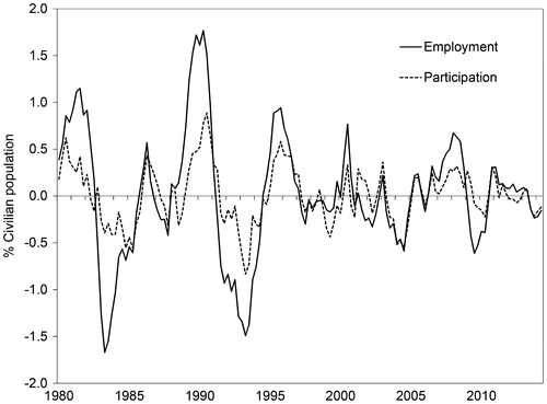
Policies intended to increase labour force participation are sometimes held out to be important against a background of an ageing population (Commonwealth of Australia 2015). Such policies cannot be framed successfully without first determining the degree to which recent changes in participation reflect transient, cyclical behaviour. We consider the existence of a business cycle component in the labour force participation rate¹ in Australia and possible theories of worker behaviour which could give rise to the observed cyclicality. In Figure 1, we compare de-trended rates of employment and total participation in Australia since 1980. Employment is considered to be procyclical since it generally rises in economic expansions and declines in contractions. There appears to be a strong positive co-movement between employment and participation rates which provides preliminary evidence that participation is procyclical.

Figure 1. Cyclical components of employment and participation.

Notes: A Hodrick-Prescott filter was used to extract the cyclical component of the employment rate and participation rate, each expressed as a percentage of civilian population.

Two theories that have been put forward to explain cyclical movement of people to and from the labour force are the so-called added-worker effect (‘AWE’) and the discouraged-worker effect (‘DWE’) (Mincer 1966). In brief, the AWE posits that workers are more likely to join the labour force during an economic contraction to compensate for actual or anticipated loss of income by other household members during the contraction, which would make a countercyclical contribution to the participation rate. The DWE works in the opposite direction. This theory posits that some unemployed workers become so discouraged at the prospect of finding a job in an economic contraction that they stop searching for work and therefore become classified as non-participating rather than unemployed. By symmetry, the same workers become encouraged to re-join the labour force during an expansion, so the DWE would make a procyclical contribution to the participation rate.

We use labour market gross flow data to look for evidence of these effects by examining the cyclicality of transition rates between the states of non-participation, employment and unemployment. First, we define a methodology for deriving transition rates from stock and flow data, and interpret the rates as revealing the probability of a person making a particular transition. Then, we look at the correlation between the transition rates and a business cycle indicator. There are four types of gross flow which affect the participation rate and we find that the AWE dominates the DWE in three of the four types. However, we find that DWE dominates the AWE in aggregate since the total participation rate is procyclical. We also construct a structural VAR (SVAR) model to examine more closely the dynamic relationship between labour market stocks and gross flows, which is useful for policy analysis.

In Section 2, we review the literature relating to AWE, DWE and cyclicality of participation. We briefly review the literature which studies transition rates between different states of employment. Section 3 describes the empirical data to be examined, including necessary transformations of gross flow data to make it compatible with stock data. The section also introduces the methodology for calculating the so-called flow rates and determining their business cycle characteristics. In Section 4, we set up a SVAR model using a mixture of gross flows, labour market stocks, job vacancies and a business cycle indicator to examine the responses of key variables to a business cycle shock. Section 5 uses impulse responses to illustrate the estimated model and in Section 6 we conclude.

2. Literature review

Mincer (1966) emphasised that the AWE and DWE should not be held as opposing theories since they can co-exist. The difficulty for our analysis is that aggregate data can only reveal which of the opposing effects is dominant but cannot necessarily reveal the contribution which each makes to the net effect. Mincer (100) found empirical evidence for a net DWE amongst the secondary workforce and evidence of the AWE amongst low-income subgroups. There have been numerous studies since Mincer which have attempted to find empirical support for both effects with mixed results, of which we mention only a small number. The AWE is often examined in the narrower context of the participation of married women conditional on the employment status of their husbands. There tends to be empirical support for the hypothesis in some developing countries including Turkey (Baslevent and Onaran 2003; Karaoglan and Okten 2012) and these findings are likely to be influenced by social norms with regard to the role of women within the countries studied. There is less evidence of the AWE in developed European countries where the DWE is usually dominant (Prieto-Rodrı́guez and Rodrı́guez-Gutiérrez 2003). Stephens (2002) uses data from a United States panel study to find evidence of the AWE in the narrow category of wives of men who have recently lost their job. Gong (2011) similarly finds evidence of the AWE for married women in Australia in the form of increased full-time employment and increased working hours. Macroeconomic time series approaches have also been used to examine participation responses of men and women to aggregate unemployment rates. Fuchs and Weber (2015) show that participation rates in Germany have had different responses to short-term and long-term unemployment rates, respectively. They find that responses to short-term unemployment imply the DWE but that long-term unemployment can be associated with the AWE in some age groups for both sexes. Benati (2001) finds evidence of countercyclical subgroups of non-participants in the United States, which he explains as a tendency amongst such workers to look for jobs only when they think they are available and who give up looking during recessions, consistent with the DWE.

For clarity we note that the terms AWE and DWE were originally coined in the context of the micro-behaviour of specific groups of workers such as wives or secondary workers. In more general use they may simply mean the behaviour of aggregate labour force participation at a business cycle frequency, as in Benati (2001, 388). Empirical evidence of procyclical participation may be interpreted as evidence that DWE dominates AWE, and vice versa if there is evidence that participation is countercyclical, as in Congregado, Golpe, and van Stel (2011). We will adopt the more general meaning of AWE and DWE in this paper in relation to the cyclicality of measures which affect participation.

There is a substantial literature which uses gross flow data to determine transition rates between employment states. The main focus of research in this literature is usually the dynamics of the unemployment rate rather than the participation rate which is our focus. Our work references previously developed techniques for extracting cyclicality of transition rates from gross flow data. Shimer (2005) focussed on transitions between employment and unemployment in the United States and found the job-finding rate to be strongly procyclical and the job separation rate to be weakly countercyclical. Hall (2006) also found that the job-finding rate was highly procyclical but that the rate of layoffs and other separations did not rise during a recession. Other authors have made findings that conflict with some of the conclusions of Shimer and Hall. Fujita and Ramey (2009) also found that the job-finding rate was highly procyclical but found that the separation rate was highly countercyclical. Yashiv (2007) found that both job-finding and job separation rates are important for understanding the business cycle. Important contributions to the analysis of transition rates in Australia have been made by Dixon, Freebairn, and Lim (2004) and Ponomareva and Sheen (2010) and we are able to compare some of our empirical results with previous findings with regard to cyclicality of transition rates.

3. Description of the data

3.1. Labour market stock variables

The period of study in this report is January 1986–June 2014. The Australian Bureau of Statistics (‘ABS’) provides monthly series of the number of employed and unemployed persons along with the participation rate and the size of the civilian population² in ABS Catalogue 6202. These series have been obtained in original as well as seasonally adjusted terms. We can determine from these series the number of civilians not participating in the labour force (referred to variously in the literature as ‘Non-participation’, ‘Not in the Labour Force’ or ‘Inactive’).

3.2. Gross flows in the labour market

Monthly gross flows of people between three labour market states of employment, unemployment and non-participation have been generated from gross changes in stocks derived from matched records in the labour force survey and published in ABS catalogue 6202, data cube GM1, for the period August 1991–December 2014. Electronic records of ABS catalogue 6203 were used to source gross flow data from January 1986 to July 1991 as originally published without adjustment. ABS catalogue 6203 does not provide data for the four monthly periods ending September 1987–December 1987 inclusive since, during that time, the ABS was implementing a transition to a new sample in the underlying survey. Linear interpolation between the corresponding months in the prior and following years was used to generate the missing data points.³

Transitions between labour market states are determined by matching respondents in consecutive monthly editions of the survey and noting their opening and closing employment status. For example, a person can be measured as having moved from employment to unemployment during the month. Due to ongoing rotation of the sample and a varying degree of non-responses each month ABS estimates that the matched records reflect only about 80% of the sample and that the final published raw data will reflect only about 80% of the population values.⁴

3.3. Transformation of gross flows

A number of transformations have been performed on the gross flow data to make it consistent with the stock data. If there were an exact correspondence between stocks and flows then first differences of a time series of stock data would equal the net difference between inflows and outflows calculated from flow data. We follow a procedure described in detail by Dixon, Freebairn, and Lim (2004) first to gross up the raw data from representing approximately 80% of the population to 100% of the population⁵ and secondly to modify individual flows to make the flow series as close as possible to being consistent with the changes in the stock data series. To use the example provided by the snapshot of raw gross flow data shown in Table 1, the gross flows between February and March are rescaled in an iterative process which seeks to match the February and March totals with those given in independent time series of stock totals for those same months. The transformed series of monthly gross flows were then seasonally adjusted using X-12-ARIMA. The monthly series are still quite noisy. Later we will compare the labour market data with a proxy variable for the output gap which is only available at a quarterly frequency, so it is convenient to simply aggregate the monthly seasonally adjusted gross flow series into an equivalent quarterly series.

Table 1. Labour force status: gross flows March 2014.

Persons (‘000)
	Labour force status March 2014
L.F. status February 2014	Employed	Unemployed	Not in the labour force	February row totals
Employed	8890.7	75.7	234.6	9201.0
Unemployed	155.8	344.0	151.1	650.9
Not in the labour force	200.8	152.8	4590.9	4944.5
March column totals	9247.3	572.5	4976.6	14,796.4

3.4. Scaling by civilian population

Many labour market studies consider the behaviour of the stock variables relative to the size of the labour force (employment plus unemployment) and in some models the size of the labour force is assumed to be constant. In our model we allow the size of the labour force to vary endogenously relative to the size of the civilian population so we rescale all of the stock variables and gross flows and express them as a percentage of the civilian population. By construction we can then make use of the identity E + U + N = 100 where E, U and N are, respectively, the number of people in employment, unemployment and non-participation divided by civilian population and multiplied by 100. For convenience we define a variable for the participation rate by PR = 100 − N. It is important to note that our definition of U is different to the conventional definition of the unemployment rate which uses the size of the labour force as the denominator. Gross flows will also be scaled by civilian population and the variables representing the flows will be in lower case letters as defined in Table 2.

Table 2. Quarterly gross flow variables.

Gross flow variable	Origin state	Destination state
eu	Employment	Unemployment
ue	Unemployment	Employment
en	Employment	Non-participation
ne	Non-participation	Employment
un	Unemployment	Non-participation
nu	Non-participation	Unemployment

3.5. Preliminary analysis of the gross flows

Figure 2 shows a diagrammatic representation of the average gross and net flows between each of the three labour market states during the sample period. We observe that the magnitude of gross flows is large in comparison to absolute net flows to or from any particular stock. It is interesting that the largest average gross flows are between the states of employment and non-participation, rather than between employment and unemployment as may have been expected. This highlights the potential advantage of a three state model which can incorporate an endogenous participation rate.

Figure 2. Summary of quarterly flows. (a) Gross flows. (b) Net flows.

Notes: Average quarterly flow as a percentage of civilian population for the sample period 1986Q1-2014Q2. Numbers in parentheses are standard deviations.

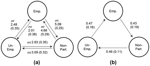
The average net flows, shown in Figure 2(b), have moved in a clockwise direction given the chosen order of nodes. It is tempting to interpret the net clockwise flow as capturing a demographic life-cycle as was noted by Dixon, Lim, and van Ours (2015, 2524), i.e. a cycle in which school leavers and other first time graduates join the workforce primarily through the unemployment pool before eventually progressing to employment and notionally replacing older workers who are moving from employment into non-participation, such as by retirement. However, since the magnitude of net flows is so much smaller than the magnitude of gross flows it is not possible to interpret the circular net flow as being representative of the transitions of any particular worker.

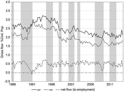
In Figure 3 we illustrate the positive comovement between flows eu and ue, both of which have tended to increase during economic contractions. For example, in the aftermath of the global financial crisis during 2008/2009 we observe that the flows eu and ue both increased, perhaps counter to an intuition that flows from unemployment to employment would fall in that period. This observation highlights the need to also consider the proportional flow, or flow rate, which takes into account the size of the pool of workers from which the flow emanates. In doing so we find that the cyclicality of flow rates may be different to the cyclicality of the corresponding gross flow.

Figure 3. Quarterly gross and net flows between employment and unemployment.

Notes: Quarterly time series of seasonally adjusted flows, 1986Q1-2014Q2. Shaded periods indicate a contraction phase of the business cycle as determined by the Melbourne Institute (n.d.).

3.6. Flow rates

We define a full period flow rate which expresses the number of workers in the gross flow as a percentage of the pool of workers from which the flow originated in the prior period. For example, we define the flow rate from the state of employment to unemployment as a percentage of employment as . Under certain conditions the flow rate is synonymous with the state transition probability of a representative individual in the originating pool. We have presented the flow rate as though it is merely a derived quantity arising as the quotient of a flow and a stock. Changes in either stocks or flows will automatically generate a change in flow rates. An alternative characterisation is one in which the flow rate and the stock level are held to be the primary quantities, whilst the flow is the derived quantity arising as the product of the stock and the flow rate. The former characterisation is more natural in our analysis since we will model stocks and flows directly. For a discussion of alternative characterisations of the relationship between stocks and flows and flow rates see Elsby, Michaels, and Solon (2009, 105–106).

3.7. Full-period and instantaneous transition rates

Gross flow data calculated from labour surveys conducted at discrete intervals will not capture multiple transitions by individuals within one measurement period so full-period transition rates will underestimate the true level of gross flows. Shimer (2012) developed a methodology to deal with this so-called time aggregation bias by calculating instantaneous transition rates which are assumed to be constant within each period. However, in this paper we will use a SVAR model to generate impulse responses corresponding to discrete full-period steps, so flow rates we derive from the impulse responses are implicitly full-period rates and will not be directly comparable with instantaneous transition rates derived by other authors.

3.8. Cyclicality of flow rates

Some empirical observations of gross flows look anomalous unless one looks at the corresponding flow rate. For example, the gross flow from unemployment to employment surprisingly tends to increase during a recession. However, the size of the pool of unemployed grows and the job-finding flow rate tends to decrease⁶ during a recession, both of which are intuitive. A representative unemployed person has a lower probability of moving to employment during the period. Even though the job-finding rate falls, the larger size of the unemployment pool results in a larger number of workers making the transition to employment.

In a similar way we can extend our intuitive understanding of each of the gross flows by examining the business cycle behaviour of the corresponding flow rates. Since flow rates reflect the probability of representative workers making a particular transition we can use the business cycle behaviour of flow rates to characterise any transitions into or out of the labour force as being consistent with either the AWE or the DWE (or neither).

We make particular definitions of AWE and DWE in the context of flow rates which are set out in Table 3 which apply to all following sections of this paper. Defined responses are only stated in the table for negative shocks to the business cycle since AWE and DWE are typically described in a recession scenario. Responses to positive shocks would have opposite sign.⁷

Table 3. Definitions of added-worker effect and discouraged-worker effect in terms of aggregate flow rates.

Defined Term	Description of the dominant behaviour	Response of specific aggregate flow rates to a negative business cycle shock	Cyclicality of flow rate
Added-Worker Effect (AWE)	An increase in the probability of workers joining, or staying in, the labour force (‘LF’) in an economic contraction.	AWE (joining LF): increase in λnu and λne	Counter-cyclical
		AWE (leaving LF): decrease in λun and λen	Procyclical
Discouraged-Worker Effect (DWE)	A decrease in the probability of workers joining, or staying in, the labour force (‘LF’) in an economic contraction.	DWE (joining LF): decrease in λnu and λne	Procyclical
		DWE (leaving LF): increase in λun and λen	Counter-cyclical

We determine the cyclicality of each of the derived flow rates using a cross-correlogram,⁸ the results of which are presented in Table 4. The cyclicality of each rate was determined solely by reference to the sign of the contemporaneous correlation coefficient between the rate and a business cycle indicator. We use a measure of the output gap as a business cycle indicator which we denote by Y. A Hodrick-Prescott filter was applied to the log of real Australian GDP data with quarterly frequency and we equated the output gap with the cyclical component of the filtered series.

Table 4. Business cycle characteristics of full-period flow rates.

Series X	Std. Dev.	Cyclicality	Cross-correlation of Y(t) with series X(t + i)
			t − 4	t − 3	t − 2	t − 1	t + 0	t + 1	t + 2	t + 3	t + 4
Flow Rates
λen	0.32	Pro.	0.22	0.19	0.23	0.24	0.26^***	0.21	0.18	0.13	0.01
λne	0.62	Pro.	0.18	0.25	0.32	0.40	0.50^***	0.52	0.45	0.42	0.24
λeu	0.25	Ctr.	−0.39	−0.55	−0.65	−0.70	−0.64^***	−0.57	−0.45	−0.30	−0.18
λue	3.83	Pro.	−0.06	0.04	0.23	0.37	0.54^***	0.58	0.57	0.51	0.40
λnu	0.42	Ctr.	−0.12	−0.24	−0.36	−0.47	−0.49^***	−0.57	−0.55	−0.47	−0.38
λun	2.81	Pro.	−0.04	0.04	0.15	0.26	0.34^***	0.47	0.54	0.55	0.46
Stocks
U	0.39	Ctr.	−0.16	−0.33	−0.48	−0.61	−0.73^***	−0.80	−0.78	−0.68	−0.53
N	0.30	Ctr.	0.23	0.14	0.05	−0.09	−0.20^**	−0.32	−0.42	−0.50	−0.54

Notes:

The cyclical component of each of the stock and flow variables was used for all calculations. Cyclicality has been determined solely by reference to the sign of the contemporaneous correlation coefficient. For the centre column *** and ** denote significance at 1 and 5%, respectively.

Table 4 shows the correlation coefficient between series Y(t) and X(t + i). For the central column with i = 0 the value is the contemporaneous correlation between Y(t) and X(t). Positive values of i mean that X(t + i) is observed after X(t). We interpret significantly positive correlations as an indicator that a series is procyclical and significantly negative correlations as an indicator that the series is countercyclical. If the correlation for X(t) has the same sign as the correlation for X(t + i), where i > 0, but the latter is larger in absolute value then we interpret this as an indicator that series X(t) lags (peaks later than) Y(t).

For comparative purposes we have placed results for the unemployment and non-participation stocks at the bottom the table. We find that unemployment is countercyclical, as would be anticipated, and lags output by one or two periods (quarters). Non-participation is also countercyclical (significant at 5%) and appears to lag output by as many as four periods. The cyclicality of participation (PR) will be the mirror image of that of non-participation. Thus, we can say that we find empirical evidence significant at 5% that PR is procyclical.

We find that is procyclical, which is consistent with our expectation, since we expect there to be an increased probability of an unemployed person finding employment during an economic expansion and a decline in a recession. Interpretation of the job separation rate is clouded by the aggregate nature of our data in which we cannot differentiate between voluntary ‘quits’ initiated by workers and ‘fires’ or ‘layoffs’ initiated by employers. Barnichon and Figura (2012, 5) find empirical support that quit rates in the United States are procyclical (as we would expect, workers to cling more tightly to current jobs in a recession) and that fires and layoffs are countercyclical (as we would expect, firms are more likely to layoff a larger portion of their workers in a recession). In our Australian data the separation rate reflects the net effect of quits and layoffs and we conjecture that the net observed counter-cyclicality of the separation rate shows that the business cycle behaviour of fires and layoffs has dominated that of voluntary quits in our sample.

These results are consistent with findings in the literature. Ponomareva and Sheen (2010, 41–44) first derive instantaneous transition probabilities from Australian gross flow data, from which they compute equivalent full period transition probabilities. They regress the transition probabilities against business cycle and recession indicator variables to assess their cyclicality. They derive results separately by gender and by full-time or part-time employment status, so their results are not directly comparable with ours. However, if we take their results for flows corresponding most closely with ours and use our notation, they find that job-finding is procyclical and that job separations to unemployment are weakly countercyclical, more so for women in the period after 1993 and for men during recessions. Elsby, Michaels, and Ratner (2015, 601) find evidence for a strongly procyclical job-finding rate and marked counter-cyclicality in the job-loss rate in the United States.

Turning our attention to flows which affect participation, Ponomareva and Sheen (2010) find that is procyclical for part-time employment and that is weakly procyclical. They find that is weakly countercyclical, significantly so only since 1993. Similarly Elsby, Michaels, and Ratner (2015, 601–604) find that in the United States and are procyclical and that is countercyclical. They do not discuss the cyclicality of directly but interpretation of their graphical presentation suggests that it tends to decline in recessions and that it is weakly procyclical.

3.9. Evidence of the DWE or the AWE

We take the empirical findings of the cyclicality of the four flow rates which affect participation from Table 4 and characterise them as being consistent with either AWE or DWE and we summarise the findings in Table 5. For example, is found to be procyclical, significant at 1%, which is consistent with AWE according to our definitions in Table 3. Our finding that the participation rate is procyclical, consistent with a net DWE, is consistent with a finding by Dixon, Lim, and van Ours (2015, 2536).

Table 5. Business cycle characteristics of participation decisions.

Rate	Characteristic cyclicality	Dominant Theoretical Effect (AWE/DWE)
Flow rate
λen	Pro.	AWE
λne	Pro.	DWE
λnu	Ctr.	AWE
λun	Pro.	AWE
Total participation	Pro.	DWE

Notes:

The cyclicality of the rates are as reported in Table 4. The cyclicality of the participation rate is the opposite of the cyclicality of non-participation.

To illustrate some of these findings more clearly consider the flow rates between non-participation and unemployment in both directions. Countercyclical is evidence that people who are currently non-participants have a higher probability (on average) of moving into unemployment (and therefore participating in the labour force) during an economic contraction, consistent with AWE. Similarly, procyclical is evidence that people who are currently unemployed have a lower probability (on average) of moving out of the labour force into non-participation during an economic contraction, which is also consistent with AWE. This could be because the unemployed person is concerned that another member of their household may lose employment due to the contraction, which increases their incentive to search for work and perhaps also to retain access to an unemployment benefit. One important conclusion which can be drawn from our findings for the flow rates between unemployment and non-participation is that the cyclicality of the flow rates in both directions contribute to a rise in unemployment during a recession, ceteris paribus. The same observation has been made by other authors including Elsby, Michaels, and Ratner (2015, 601) in relation to the United States.

It is intriguing that AWE dominates DWE on three of the four transitions shown in Table 5, yet the behaviour of the overall participation rate is dominated by DWE. This is likely to be due to the gross flow ne dominating the overall cyclicality of the participation rate since it is the second largest gross flow on average and its cyclical component is the most volatile of any of the flows.

Our preliminary analysis has shown that it is possible, using only aggregate data, to identify whether the dominant behaviour is consistent with AWE or DWE in each of the four types of flow that directly affect participation. However, correlations can only reveal a limited amount of information about the dynamic interaction between the variables. In Section 4 we will use a SVAR model to assist in classifying the cyclicality of flow rates by examining the dynamic responses of flow rates to orthogonalised shocks to the business cycle indicator.

4. SVAR model

4.1. Mixed model using stocks and flows

We set up a SVAR model with a mixture of stocks, job vacancies and gross flows as endogenous variables. It seems highly likely that there would be two-way causal relationships between stocks and flows if the true underlying processes were known. By definition, gross flows to or from a stock will cause contemporaneous change in the level of that stock. However, theory does not provide a guide to expected indirect or lagged effects of flows on stocks. Considering possible causation in the other direction, we expect lagged values of stock variables to affect gross flows (e.g. the unemployment stock in the last period may affect the current period flow out of unemployment). The full period flow rate from state A to state B in the period from time t to (t + 1) will be derived as , where ab(t + 1) is the gross flow of people during the period from t to (t + 1) and A(t) is the number of people in state A at time t. This can be expressed equivalently as , which illustrates that flows should be linked to lagged stock values rather than contemporaneous values. This can be achieved in the SVAR model within a recursive structure which places gross flows above the stock variables so that changes to gross flows can have a contemporaneous effect on stocks, but not vice versa.

There are few examples in the literature which have applied a SVAR model to labour market flows. In a recent paper Dixon, Lim, and van Ours (2015) use a SVAR model to analyse how shocks to net flows affect the evolution of the Australian unemployment rate and participation rate. The dimension of the model is reduced since there only three net flows rather than six gross flows. The authors derive theoretical relationships between net flows and rates of participation, employment and unemployment and use these identities to trace out implied responses of these rates to shocks applied in the SVAR model. A possible limitation of using this approach in policy analysis is that there is not a one-to-one relationship between net flows and policy interventions, as noted by Dixon, Lim, and van Ours (2015, 2533). For example, separate policies to either protect existing jobs or to encourage hiring unemployed workers will both affect the net flow between employment and unemployment. We demonstrate that it is possible to construct a SVAR model which uses gross flows which could be used to examine the implications of policies or shocks which directly affect a flow in only one direction. A similar aspect of our approach to that used by Dixon, Lim and van Ours is that we make use of identity relationships to generate the implied responses of other variables not included directly in the SVAR model, which we explain in a following section.

4.2. Selection of variables

We have four identities by which certain stocks and gross flows are related, as follows:

(1)

(2)

(3)

(4)

We cannot include all three of E, U and N in the VAR model since they are related by the identity described by Equation (1(1) ). We will include E and U since they have the strongest theoretical links to other macroeconomic variables. It is straightforward to determine the implied response of N using Equation (1(1) ) given impulse responses for E and U. By similar reasoning we cannot include all six of the gross flows in a VAR model which already includes two of the stock variables and their lagged values since there are identity relationships between changes in stocks and gross flows as described by Equations (2(2) ) to (4(4) ). In particular, we cannot include all four gross flow variables that go into or come out from a particular stock. We will include the set eu, ue, ne and nu in the model, the first two of which were included because they are usually of most interest in labour market economics. The choice of the remaining two flow variables was arbitrary.⁹ We can also determine the implied responses of the remaining two gross flow variables using the identities. Finally, using the implied responses of flows and stocks, we can calculate implied responses of all six of the flow rates.

We also included the level of job vacancies¹⁰ (V) in the model since there is a long history of literature indicating that vacancies can play a significant role in the propagation of shocks through the labour market, in particular to the level and persistence of unemployment. There is a direct theoretical link between vacancies and gross flows into employment (for a detailed discussion of micro-foundations of search and matching theory see Cahuc and Zylberberg [2004], Blanchard and Diamond [1989] and Pissarides [1986]).

The model contains a mixture of stationary and non-stationary variables. The business cycle indicator Y will be stationary since it was extracted as the cycle component of a Hodrick-Prescott decomposition. Most of the other stock and flow variables exhibited non-stationary behaviour in the sample period. We estimated the model in levels of the variables (without differencing or de-trending) following the argument made by Stock and Watson (1988) that important information about the dynamic relation between the series may be contained in the levels rather than in the differences. Stock and Watson set out conditions under which it would still be possible to draw inferences about coefficient estimates from a model with a mixture of stationary and integrated variables but that is not an objective in the current study. We will focus on the interaction between the variables as revealed by impulse responses rather than coefficient estimates.

4.3. Structural model

We will estimate a structural model of the form B(L)X_t = ɛ_t, where X_t is a (8 × 1) vector of endogenous variables, L is the lag operator and B(L) = B₀ − B₁L − B₂L² − … − B_pL^p. The lag order is p. We used a likelihood ratio test to compare one lag against an alternative of two, and two against an alternative of three (Doan 2012, UG209). Test results supported the choice of two lags. The matrix B₀ captures the coefficients for the contemporaneous interactions between the variables, and the matrices B_i capture the coefficients at lag i for i > 0. The structural errors ɛ_t have zero mean and are serially uncorrelated. We will use a recursive identification scheme with a lower triangular form for the matrix B₀. It is well known that by imposing a recursive structure on the contemporaneous coefficient matrix we can estimate the reduced form of the system using ordinary least squares working in order from the first row down to the last. The recursive structure also provides the condition for exact identification of the model so that we can recover the coefficients in B₀. A description of methodology for estimating a recursive VAR model can be found in Enders (2010, 297–307).

4.4. Recursive identification scheme

The cyclical component of the output gap has been used as a proxy for the business cycle indicator in the SVAR model so that we may directly measure the response of the labour market variables to unexpected shocks in the business cycle. We have placed Y in the first row of the vector of variables based on the assumption that all the variables following in the order may respond contemporaneously to a business cycle shock. Y is endogenous in the model so that feedback of lagged responses of labour market stocks and flows can affect Y. We described earlier that gross flows are related to lagged values of stock variables so flows are placed above stocks in the model, in the order eu, ue, ne, nu. We relied primarily on leads and lags in cross-correlogram analysis to determine the order amongst the flow variables since there is no theory to guide the ordering. Search and matching theory supports placing vacancies first amongst the stock variables because firms choose the level of vacancies to supply in a forward looking manner (Cahuc and Zylberberg 2004, 546) so we chose the order V, E, U for the last three stock variables. We experimented with some alternative non-recursive schemes using restrictions suggested by empirical analysis but were not able to find any material benefit to justify using a more complicated scheme.

4.5. Initial conditions for steady state

Even if the labour stock variables were in steady state there is no unique combination of steady state values for the gross flow variables. We provide our own definition of steady state for the system and set initial values for the stocks and flows to achieve it. Then impulse responses can be interpreted as movements away from an initial steady state. We define an equilibrium state as one in which the labour stock variables are unchanged from one period to the next, which implies that net inflows and outflows have offset one another. The simplest way to achieve such a state is one in which there is a constant (possibly zero) circular flow between the three states.¹¹

In Figure 2(b) we showed that the sample mean quarterly net flows between each pair of states were within the narrow range 0.43–0.47% of civilian population. For initial conditions approximating a steady state equilibrium we set all of the included model variables to their sample mean values and we chose initial values of the excluded variables en and un to generate a constant clockwise circular net flow of 0.47%. Given initial values for all the variables and a set of impulse responses we are able to derive implied impulse responses of the flow rates.

5. Estimation results: impulse responses

Parameter estimates are not provided here since individual parameter estimates typically have no direct interpretation when there are a large number of variables in a VAR model. We focus on interpreting the impulse response functions (‘IRFs’) of the variables to shocks to the structural errors (good explanations of IRFs can be found in Enders [2010, 307–315] and Hamilton [1994, 318–324]). It is typical to plot the responses against the period index and to interpret the resulting IRF as the evolution of the dependent variable through time following a one-time shock in the first period.

5.1. Output shock

In Figure 4 we plot impulse responses of selected model variables to a positive one standard deviation shock lasting for one period to the orthogonal error term in the first equation (‘output shock’). The response of Y shows the inherent persistence that is typical in macroeconomic variables with the level of Y remaining above its equilibrium level for almost two years. E and U show procyclical and countercyclical responses, as expected, for about two years before reverting to and overshooting their initial equilibrium levels. We illustrate the implied impulse response of the participation rate PR which has been derived using the appropriate identity relationship. The direction of the response of PR is consistent with procyclical behaviour but the magnitude is very small. At most the response of PR could be described as weakly procyclical. The point estimates of the response of vacancies appear to be negatively correlated with unemployment, as we would expect from a theoretical Beveridge curve relationship (Cahuc and Zylberberg 2004, 512), but the error bands are wide and the result is not significant.

Figure 4. Impulse responses of selected variables: Y shock.

Notes: One standard deviation shock to the structural error term. Confidence bands are displayed at ±2 SE around the point estimates, and are only available for variables included directly in the model.

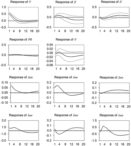
We show impulse responses of the flow rates which are derived from the response paths of the relevant gross flows and stock variables. The job-finding rate is elevated for two years in line with an intuitive response to a positive output shock, which we interpret as meaning that is procyclical. The response of the job separation rate is ambiguous. The rate falls initially by a negligible amount but then rises steadily. However, the rate does not become materially positive until the second year, during which time the initially positive responses of Y and E have already been eroded and are becoming negative. The cyclicality of the job separation rate is not clearly determined by this test.

Our main interest is the cyclicality of the flow rates relating to participation, which are more clearly determined from the impulse responses and which are consistent with our earlier findings using the cross-correlogram as set out in Table 5. For example, rises in response to a positive business cycle shock which lasts about eight periods so the empirical evidence is that is procyclical. To summarise, we find that each of , and are procyclical whilst is countercyclical. According to the definitions set out in Table 3, these results are consistent with AWE being dominant for , and whilst DWE is dominant for . That means that there is an increased tendency of non-participants to join unemployment during an economic contraction and a reduced tendency of unemployed workers to leave the labour force. However, at the same time overall non-participation has generally risen during contractions mostly due to a reduced tendency of non-participants to move into employment.

6. Conclusion

The business cycle characteristics of flow rates between labour market states are measured using correlation analysis and a SVAR model and the results are used to characterise flows into and out of the labour force as being consistent either with the AWE or the DWE. We find evidence that the AWE is dominant in transitions in both directions between unemployment and non-participation which contributes to a rise in unemployment during contractions. We also find that the DWE is dominant in transitions from non-participation to employment and that this drives the overall result that non-participation rises during a contraction. It is important to be able to measure the cyclical influences on labour force participation and its interaction with unemployment before attempting to frame policy responses to perceived slack in the labour market.

Disclosure statement

No potential conflict of interest was reported by the author.

Notes

1. The labour force is the sum of employed and unemployed persons. The participation rate is the percentage of the civilian population in the labour force.

2. Civilians aged 15 years and over.

3. These estimates will affect two of 114 quarterly observations in relevant regression analysis that follows in this report.

4. See ABS 6102.0.55.001 – Labour Statistics: Concepts, Sources and Methods, 2013, Chapter 20 Labour Force Survey.

5. The process of grossing up the size of the sample from 80 to 100% is only valid if the missing respondents had the same distribution of transition characteristics as the remaining 80% from which they are estimated. The ABS estimates that only about two thirds of the unmatched 20% portion is likely to have similar characteristics to the matched group.

6. We will show this empirical result in a following section.

7. We avoid switching to new terminology for responses under positive shocks to the business cycle as may occur sometimes in the literature, such as ‘subtracted-worker effect’ and ‘encouraged-worker effect’. These represent the same psychological behaviour as AWE and DWE, respectively, simply operating in the alternate phase of the business cycle.

8. We follow a format used by Fisher, Otto, and Voss (1996).

9. We tried different combinations of variables without finding material differences in impulse responses.

10. Job Vacancies Australia (total) series from ABS Catalogue 6354. The series has a gap from August 2008 to August 2009 during which time the survey was not conducted. A quintic spline was used to generate the missing points.

11. This mirrors the device used by Dixon, Lim, and van Ours (2015, 2527) to achieve equilibrium with equal circular net flows.

References

- Barnichon, Regis, and Andrew Figura. 2012. “The Determinants of the Cycles and Trends in US Unemployment.” Unpublished manuscript, CREI, Universitat Pompeu Fabra and Barcelona GSE.
- Baslevent, Cem, and Ozlem Onaran. 2003. “Are Married Women in Turkey More Likely to Become Added or Discouraged Workers?” Labour 17 (3): 439–458.10.1111/labr.2003.17.issue-3
- Benati, Luca. 2001. “Some Empirical Evidence on the ‘Discouraged Worker’ Effect.” Economics Letters 70 (3): 387–395.10.1016/S0165-1765(00)00375-X
- Blanchard, Olivier Jean, and Peter Diamond. 1989. “The Beveridge Curve.” Brookings Papers on Economic Activity 1989: 1–76.10.2307/2534495
- Cahuc, P., and A. Zylberberg. 2004. Labor Economics. Cambridge, MA: The MIT Press.
- Commonwealth of Australia. 2015. 2015 Intergenerational Report: Australia in 2055. Canberra: Commonwealth of Australia.
- Congregado, Emilio, Antonio A. Golpe, and André van Stel. 2011. “Exploring the Big Jump in the Spanish Unemployment Rate: Evidence on an ‘Added-Worker’ Effect.” Economic Modelling 28 (3): 1099–1105.10.1016/j.econmod.2010.11.018
- Dixon, Robert, John Freebairn, and Guay C. Lim. 2004. “A Framework for Understanding Changes in the Unemployment Rate in a Flows Context: An Examination Net Flows in the Australian Labour Market.” Research Paper 910, University of Melbourne Department of Economics.
- Dixon, Robert, Guay C. Lim, and Jan C. van Ours. 2015. “The Effect of Shocks to Labour Market Flows on Unemployment and Participation Rates.” Applied Economics 47 (24): 2523–2539.10.1080/00036846.2015.1008771
- Doan, Thomas. 2012. RATS User’s Guide, Version 8.2. Evanston, IL: Estima.
- Elsby, Michael, Ryan Michaels, and David Ratner. 2015. “The Beveridge Curve: A Survey.” Journal of Economic Literature 53 (3): 571–630.10.1257/jel.53.3.571
- Elsby, Michael W. L., Ryan Michaels, and Gary Solon. 2009. “The Ins and Outs of Cyclical Unemployment.” American Economic Journal: Macroeconomics 1 (1): 84–110.
- Enders, Walter. 2010. Applied Econometric Time Series. 3rd ed. New Jersey: Wiley.
- Fisher, Lance A., Glenn Otto, and Graham M. Voss. 1996. “Australian Business Cycle Facts.” Australian Economic Papers 35 (67): 300–320.10.1111/j.1467-8454.1996.tb00052.x
- Fuchs, J., and E. Weber. 2015. “Long-term Unemployment and Labor Force Participation.” IAB-Discussion Paper, 32.
- Fujita, Shigeru, and Garey Ramey. 2009. “The Cyclicality of Separation and Job Finding Rates.” International Economic Review 50 (2): 415–430.10.1111/iere.2009.50.issue-2
- Gong, Xiaodong. 2011. “The Added Worker Effect for Married Women in Australia.” Economic Record 87 (278): 414–426.10.1111/ecor.2011.87.issue-278
- Hall, Robert E. 2006. “Job Loss, Job Finding and Unemployment in the US Economy over the past 50 Years.” In NBER Macroeconomics Annual 2005, 101–166. Vol. 20. MIT Press.
- Hamilton, James Douglas. 1994. Time Series Analysis. Princeton, NJ: Princeton University Press.
- Karaoglan, Deniz, and Cagla Okten. 2012. “Labor Force Participation of Married Women in Turkey: Is There an Added or a Discouraged Worker Effect?” Discussion Paper No. 6616, Forschungsinstitut Zur Zukunft Der Arbeit.
- Melbourne Institute. n.d. “Phase of Business Cycles, Australia 1960–2015.” The University of Melbourne. Accessed February 10, 2016. http://melbourneinstitute.com/macro/reports/bcchronology.html
- Mincer, Jacob. 1966. “Labor-force Participation and Unemployment: A Review of Recent Evidence.” In Prosperity and Unemployment, edited by Robert Aaron Gordon and Margaret S. Gordon, 73–112. New York, NY: Wiley.
- Pissarides, Christopher. 1986. “Unemployment and Vacancies in Britain.” Economic Policy 1 (3): 499–541.10.2307/1344583
- Ponomareva, Natalia, and Jeffrey Sheen. 2010. “Cyclical Flows in Australian Labour Markets.” Economic Record 86 (s1): 35–48.10.1111/j.1475-4932.2010.00658.x
- Prieto-Rodrı́guez, Juan, and César Rodrı́guez-Gutiérrez. 2003. “Participation of Married Women in the European Labor Markets and the ‘Added Worker Effect’.” The Journal of Socio-Economics 32 (4): 429–446.10.1016/S1053-5357(03)00050-7
- Shimer, Robert. 2005. “The Cyclical Behavior of Equilibrium Unemployment and Vacancies.” American Economic Review 95: 25–49.10.1257/0002828053828572
- Shimer, Robert. 2012. “Reassessing the Ins and Outs of Unemployment.” Review of Economic Dynamics 15 (2): 127–148.10.1016/j.red.2012.02.001
- Stephens Jr., Melvin. 2002. “Worker Displacement and the Added Worker Effect.” Journal of Labor Economics 20 (3): 504–537.10.1086/339615
- Stock, James H., and Mark W. Watson. 1988. “Variable Trends in Economic Time Series.” Journal of Economic Perspectives 2 (3): 147–174.10.1257/jep.2.3.147
- Yashiv, Eran. 2007. “U.S. Labor Market Dynamics Revisited.” Scandinavian Journal of Economics 109 (4): 779–806.10.1111/j.1467-9442.2007.00521.x