Spatial distribution patterns of benthic macroinvertebrate functional feeding groups by stream size and gradient in Republic of Korea

Abstract

Benthic macroinvertebrate functional feeding groups (FFGs) are influenced by the availability of food sources, which can be affected by stream size and gradient. We investigated the spatial distribution patterns of FFGs by stream size (stream order, catchment area and stream width) and gradient (altitude and slope). In addition, we attempted stream classification based on the distribution patterns of FFGs. To achieve these goals, a total of 996 sampling sites of national scale located in the Republic of Korea were investigated from 2008 to 2016. Among the five physical variables, stream width and slope showed linear relationships with the indicator values of FFGs. These two physical variables had larger influences on the distribution of FFGs compared to other variables. Geology (the type of rocks) showed little influences on the distribution of benthic macroinvertebrate communities. We classified streams focusing on catchment (stream size) area and altitude (stream gradient) because they are constants that do not change with disturbances. The FFGs and benthic macroinvertebrate assemblages were distinctly changed by stream types, indicating that the stream classification criterion adequately represented changes in physical variables in biotic terms. In addition, the distribution of FFGs and biotic assemblages showed that benthic macroinvertebrates in the Republic of Korea were more influenced by the altitude (stream gradient) than the catchment area (stream size). In overall, this study found that the stream size and gradient markedly influence the distribution of FFGs in national regions of the Republic of Korea. Further research is needed focusing on the level of microhabitats and other parameters to identify the promising variables that influence biotic distribution.

Keywords:

• Benthic macroinvertebrates
• functional feeding groups
• Republic of Korea
• stream classification
• stream gradient
• stream size

Introduction

It is important to elucidate the variation in benthic macroinvertebrates diversity and their functional role in order to gain insight into the underlying abiotic and biotic variables that generate various patterns in stream ecosystems (Li et al. 2012). Among the several aquatic organisms present in streams or rivers, benthic macroinvertebrates have a differentiated functional form according to the given physical or chemical conditions. Thus, their species diversity is high and responds to changes in the various environmental variables (Jun et al. 2016; Kim et al. 2016). Based on these characteristics, benthic macroinvertebrates have been used as bioindicators for assessment of water quality and the health of aquatic environments (Rosenberg et al. 1986; Smith et al. 1999; Barman and Gupta 2015).

Benthic macroinvertebrates play an important role in the functional aspects of lotic ecosystems such as control of primary production, detritus breakdown and nutrient mineralization (Merritt and Cummins 1996; Wallace and Webster 1996). For examples, they consume primary producers and are consumed by fishes, forming part of the food chain and transferring energy to higher levels (Cummins 1973; Wallace and Webster 1996; Glaz et al. 2012). In addition, they serve as decomposers of organic matter, which is broken and consumed into smaller pieces and excreted to form food for other consumers such as microorganisms, resulting in microbial decomposition (Wallace and Webster 1996; Fenoglio et al. 2002; George et al. 2010). With a focus on the importance of these ecological functions, Cummins (1974) grouped benthic macroinvertebrates into functional feeding groups (FFGs). These were classified based on the types of food sources and feeding behavior mechanisms as opposed to species morphological characteristics (Cummins 1973; Cummins and Klug 1979; Merritt and Cummins 1996). FFGs were classified as shredders, scrapers, collectors (filterers or gatherers) and predators (Cummins 1973; Merritt and Cummins 1996). Shredders mainly feed on coarse particulate organic matter (CPOM) such as leaf litter which is then, transform it into fine particulate organic matter (FPOM). Scrapers feed on periphyton which is found on the surface of coarse substrates. Furthermore, collectors feed on FPOM from the water column (filterers) or streambed (gatherers), and predators consume live prey (Cummins and Klug 1979; Merritt and Cummins 1996; Wallace and Webster 1996).

FFGs have been described as key components in the river continuum concept (RCC; Vannote et al. 1980). Shredders, scrapers and collectors have shown distinct distribution patterns according to the stream size compared to other FFGs (Vannote et al. 1980). The distribution of FFGs is significantly influenced by food sources and availability, which can be changed with stream size (Allan and Castillo 2007), but specific taxa belonging to each FFG is considered to reflect the effects of disturbances. Generally, shredders and scrapers have more sensitive taxa to disturbances that might change the availability of certain food or habitat, while collectors (filterers and gatherers) are more tolerant, so they can potentially be used to assess aquatic ecosystem health (Bhawsar et al. 2015). Thus, considering the importance of FFGs in biomonitoring, assessment of the functional organization of benthic macroinvertebrate assemblages is essential (Príncipe et al. 2010). For this reason, studies on the distribution of FFGs and benthic macroinvertebrate assemblages according to environmental variables are increasingly being conducted (Brasil et al. 2014; Barman and Gupta 2015; Bhawsar et al. 2015; Fierro et al. 2015; Fu et al. 2016).

A stream can continuously change its natural structure and function as water flows from upstream to downstream along the longitudinal gradient (Allan and Castillo 2007). Accordingly, continuous changes in various environmental variables due to the longitudinal gradient of stream are accompanied by changes in benthic macroinvertebrate assemblages. Among the various environmental variables, there are a number of physical variables that can influence benthic macroinvertebrate fauna regardless of water quality, which include stream order, catchment area, stream width, altitude, slope, geology, flow velocity, and streambed composition (Nelson and Lieberman 2002; Heino et al. 2005; Merz and Ochikubo 2005; Jiang et al. 2010; Li et al. 2012; Jun et al. 2016; Kim et al. 2017). These physical variables also influence the distribution of FFGs by altering the food types. Riparian vegetation in upstream reduces primary production due to shading, but at the same time it serves as the main allochthonous organic material. Shredders have a high distribution ratio in upstream because they mainly use allochthonous CPOM like fallen leaves. As stream size increases, the influence of riparian vegetation decreases, which in turn increases the input of organic material from upstream and autochthonous primary production. Also, the increase in primary production leads to an increase in scrapers in the midstream. There is little influence of riparian vegetation in downstream. However, organic material from upstream or midstream mainly consumed downstream due to the effects of water depth and turbidity that may limit primary production. Since most of the organic material is in the state of FPOM by shredders or scrapers, the share of collectors is increased in downstream (Vannote et al. 1980).

This article investigated the distribution patterns of FFGs according to stream size and gradient on the national scale based on the RCC. The distribution of FFGs according to physical variables in the Republic of Korea was reported by Kim et al. (2017). However, this study (1) confirmed the distribution of FFGs by adding sampling size (2,297), catchment area and slope that were not considered in the previous study, (2) set a biotic indicator using FFGs rather than distribution ratio of each FFG, (3) analyzed whether geology affects benthic macroinvertebrate communities. Finally, (4) we classified each physical variable based on the distribution patterns of FFGs and attempted stream classification using comprehensive analysis results.

Materials and methods

Study area

This study was conducted in the mainstems, tributaries and other independent streams of five major river watersheds (Han, Nakdong, Geum, Yeongsan and Seomjin Rivers) of national scale in the Republic of Korea. The total number of sampling sites was 996 (15,663 sampling size; Figure 1).

Figure 1. Location of the 996 sampling sites in the Republic of Korea. The black thick lines indicate the four major river (Han, Nakdong, Geum and Yeongsan-Seomjin Rivers) watersheds while the light thin lines display the main and tributaries of five rivers and other independent rivers. White circles, black squares and gray squares respectively represent all sampling sites, the reference streams of Bukhan River and the reference streams of Namhan River.

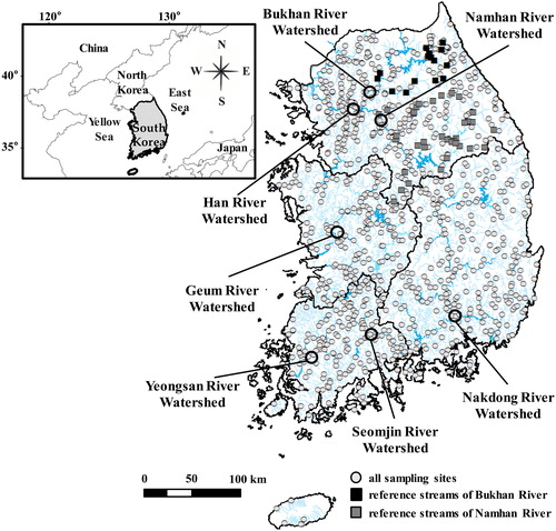
Since the topography of the Republic of Korea mostly consists of mountainous areas, mountain streams occupy a larger area than plain streams (Bae et al. 2003). In addition, there are many high mountains in the eastern part of the country. Thus, the east is formed by steep slopes while the west consists of lowland plains as the altitude decreases (Lee et al. 2011).

Geology can be simply divided into granite and limestone zones. Granite zones occupy most of the total land area, while limestone zones only occur in certain areas (Yun and Moon 2009). The Han River can be divided into the Namhan River (south Han River) and Bukhan River (north Han River), which are a typical limestone zone and a granite zone, respectively (Kim and Shim 2001; Ryu et al. 2008).

Measurement of environmental variables

The environmental variables used in this study included physical variables and geological variables (geology). The physical variables were stream order, catchment area (km²), stream width (m), altitude (m) and slope (%). Stream order (Strahler 1957) was determined using a 1:25,000 scale map. Catchment area was determined using the Korean Reach File provided by NIER (2015). Stream width was determined by measuring the distance between bank to bank at the sampling sites using a laser range finder (Bushnell Inc., Overland Park, KS, USA). Altitude at the sampling sites was measured using GPS (Triton 500, Magellen Inc., San Dimas, CA, USA). Slope was calculated using ArcGIS (ESRI, version 10.2) software. The elevation difference between two points (500-m upstream and 500-m downstream from a sampling site) was divided by the distance (1000 m), then multiplied by 100 (Parsons et al. 2001; Ministry of Environment [ME] 2011).

Geology ultimately influences biota as it affects water chemistry in terms of hardness and buffer action (Olivero and Anderson 2008). Since limestone zones have higher contents of calcium and magnesium ions as well as acid-neutralizing capacity than granite zones, they have higher conductivity (dS/m) and pH levels (Yun and Moon 2009). Thus, conductivity and pH were used as variables to represent geology. These were measured at sampling sites using multiprobe portable meters (e.g. YSI 6920, YSI Inc., Yellow Springs, OH, USA or Horiba U-22XD, Kyoto, Japan).

Sampling of benthic macroinvertebrates

The sampling procedure and sample analysis methods were carried out according to the guideline of ME and NIER (2013). Benthic macroinvertebrates were collected at 996 sampling sites using a Surber sampler (30 cm $\times$ 30 cm, 1 mm mesh). Sampling was conducted randomly within 100 m of sampling sites, mainly based on fast-flowing riffle or glide-run habitats (when suitable riffles were unavailable; Jun et al. 2016). Quantitative samples with three replicates (0.27 m² of habitat for each sampling unit) were collected in spring and autumn (some were only collected once per year in either spring or autumn) every year at each site. Following field sampling, the collected samples were fixed with 95% ethanol, transferred to the laboratory, sorted from detritus and inorganic materials and finally stored in 80% ethanol. The specimens were identified to the species level if possible. Some taxa with limited taxonomic information (e.g. Oligochaeta, Gammaridae and Chironomidae) were identified to the genus or family level. All individuals were counted and converted to individual abundance/m². Further, all benthic macroinvertebrate specimens were assigned to suitable FFGs according to Cummins et al. (2005), Merritt and Cummins (1996), and Ro and Chun (2004; Appendix 1).

Data analysis

Stream order, catchment area, stream width, altitude, and slope can change continuously with the longitudinal gradient. However, geology is simply classified by the type of rock material. Thus, geology was considered to be a variable independent from the other five variables, and the effects of geology and the other five variables on biotic communities were confirmed by different analyses.

Pearson correlation analysis and principal component analysis (PCA) were conducted to determine relationships among the five physical variables as well as identify the attributes of each physical variable. Prior to PCA, each physical variable was adjusted in the range of 0 to 1 based on minimum–maximum range normalization, because the range of variable values differed (Hwang et al. 2011; Jun et al. 2016). The raw values of each physical variable may show normality, while some of the physical variables do not show normality. The normality for raw values of physical variables was checked, and the variables that did not show normality were transformed to $\ln (x+1).$ Based on the data values showing normality, each variable was then calculated using the following Equation (1)(1) $$A_1=(V_x-V_{\min })/(V_{\max }-V_{\min })$$(1) . Finally, PCA was conducted using adjustment values ($A_1$). (1) $$A_1=(V_x-V_{\min })/(V_{\max }-V_{\min })$$(1)

According to the RCC, among the benthic macroinvertebrate FFGs, shredders, scrapers, collectors have distinct distribution characteristics by stream size (Vannote et al. 1980; Bhawsar et al. 2015). Based on this concept, we used the biotic indicator value to analyze the distribution pattern of FFGs for each physical variable aside from geology. The individual abundance of FFGs was transformed to $\ln (x+1)$ in order to downweigh the effect of dominant taxa by particular taxa (e.g. Chironomidae and Baetidae: collectors; Jun et al. 2016). Using Equation (2)(2) $$I=\ln \left(\mathrm{CF}+\mathrm{CG}\right)/\ln \left(\mathrm{SH}+\mathrm{SC}\right)={\log }_{\left(\mathrm{SH}+\mathrm{SC}\right)}(\mathrm{CF}+\mathrm{CG})$$(2) shown below, the ratio of the individual abundance of collectors (filterers and gatherers) was transformed to $\ln (\mathrm{CF}+\mathrm{CG}),$ while the individual abundance of shredders and scrapers was transformed to $\ln (\mathrm{SH}+\mathrm{SC})$ as a biotic indicator value ($I$) of FFGs. When analyzing the relationship between physical variables and indicator values, the regression analysis results may be distorted if the sampling sites are concentrated in a range of specific environmental variables. To avoid this issue, each environmental variable was divided into equal intervals, then the mean and cumulative mean indicator value were obtained for each interval. The relationship between the class mark of each physical variable and indicator value was analyzed to confirm the distribution patterns of FFGs, and based on these, the relationships of each physical variable were classified. (2) $$I=\ln \left(\mathrm{CF}+\mathrm{CG}\right)/\ln \left(\mathrm{SH}+\mathrm{SC}\right)={\log }_{\left(\mathrm{SH}+\mathrm{SC}\right)}(\mathrm{CF}+\mathrm{CG})$$(2)

In order to determine whether geology could influence the distribution of benthic macroinvertebrate communities, the Han River was divided into the Namhan River (limestone) and the Bukhan River (granite). Canonical correspondence analysis (CCA; Ter Braak 1986) was then conducted using biotic communities, conductivity and pH. At this time, it was necessary to assume that the benthic macroinvertebrate communities in the Namhan River and the Bukhan River were not influenced by environmental variables other than conductivity and pH. Thus, the influence of geology was analyzed using data from a reference stream selected by ME (2017) among the 996 sampling sites. To determine the differences in conductivity and pH between the Namhan River and the Bukhan River, we used t-tests. The individual abundance of benthic macroinvertebrates used for CCA was also transformed to adjustment values ($A_2$) following Equation (3)(3) $$A_2=0.5+(\ln n-\ln n_{\min })/(\ln n_{\max }-\ln n_{\min })=0.5+{\log }_{(n_{\max }/n_{\min })}(n/n_{\min })$$(3) , so the effects of dominant taxa were downweighted and the range of individual abundance of each taxon was equal (Hwang et al. 2011; Jun et al. 2016). Conductivity and pH were also checked for normality, pH which was used as the raw value, but conductivity was transformed to $\ln (x+1).$ (3) $$A_2=0.5+(\ln n-\ln n_{\min })/(\ln n_{\max }-\ln n_{\min })=0.5+{\log }_{(n_{\max }/n_{\min })}(n/n_{\min })$$(3)

Based on the results of the above analysis, after confirming the relationship between biotic and physical variables, the streams were classified using only the variables that affect the biotic distribution. In addition, benthic macroinvertebrate assemblages were analyzed for each classified stream in order to determine whether stream classification focused on the distribution of FFGs was appropriate or not.

PCA and CCA were performed using PC-ORD (MjM software, version 6.19, Glenede Beach, OR, USA). Pearson correlation analysis and the t-test were conducted using PASW (for Windows 8, version 6.3 and SPSS Inc., Chicago, IL, USA).

Results

Overall condition of physical variables at sampling sites

The sampling sites were varied from small to large as well as from high-altitude and steeply sloped to low-altitude and gently sloped streams (Table 1). In terms of stream order and catchment area, there were only 4 first-order streams and 10 streams with area less than 3 km², so there were very few headwater streams. In addition, in first-order streams, the narrowest stream width was 10 m, and the narrowest stream was third-order stream. Thus, it was shown that the smaller size of the stream, the more different size of the stream can be according to the physical variables it uses, depending on the shape of the stream. The mean of most physical variables was larger than the median, indicating that the sampling sites were concentrated in relatively small, low-altitude streams. Of the 996 sampling sites, the total number of sites in the Namhan River and the Bukhan River was 258 (Namhan River, 165; Bukhan River, 93). However, only 52 sites (Namhan River, 37; Bukhan River, 15) were selected as reference streams. The conductivity and pH of the Namhan River were significantly ($p<0.01$) different (specifically, higher) than those of Bukhan River (Table 1).

Table 1. Summary of environmental variables representing (a) stream size and (b) gradient in the 996 sampling sites and (c) geology as the reference stream.

Variables		Mean	SD	Med	Min – Max	No of sites	$p$ (t-test)
(a) Stream size
Stream order		5.0	2.0	5.0	1.0 – 9.0	996	–
Catchment area (km^2)		765.7	2333.1	90.3	1.2 – 23376.5		–
Stream width (m)		131.2	147.0	82.5	5.3 – 1260.0		–
(b) Stream gradient
Altitude (m)		137.0	157.3	77.6	0.0 – 888.0	996	–
Slope (%)		7.6	6.1	6.0	0.0 – 27.8		–
(c) Geology
Conductivity (dS/m)	RSNR	0.160	0.062	0.163	0.034 – 0.314	37	0.000
	RSBR	0.085	0.023	0.078	0.054 – 0.141	15
pH	RSNR	7.9	0.4	7.9	7.0 – 8.6	37	0.003
	RSBR	7.5	0.3	7.5	7.1 – 8.0	15

Max: maximum; Med: median; Min: minimum; No of sites: number of sites; RSBR: reference streams of Bukhan River; RSNR: reference streams of Namhan River; SD: standard deviation.

Relationship between physical variables

Pearson correlation analysis was conducted to determine the relationships between each physical variable aside from geology (Table 2). Stream order, catchment area and stream width shown significantly high correlations with each other. The highest correlation was found between stream order and catchment area ($r=0.912,\mathrm{ }p<0.01$). In contrast, these variables showed low correlations with altitude and slope. The correlation between altitude and slope ($r=0.643,\mathrm{ }p<0.01$) was found to be high and significant. However, it was lower than the correlations among stream order, catchment area and stream width.

Table 2. Pearson correlation coefficient (r) between each physical variable.

	Stream order	Catchment area (km^2)	Stream width (m)	Altitude (m)
Catchment area (km^2)	0.912**	–	–	–
Stream width (m)	0.831**	0.873**	–	–
Altitude (m)	–0.324**	–0.328**	–0.412**	–
Slope (%)	–0.297**	–0.361**	–0.419**	0.643**

^** $p$ value < 0.01.

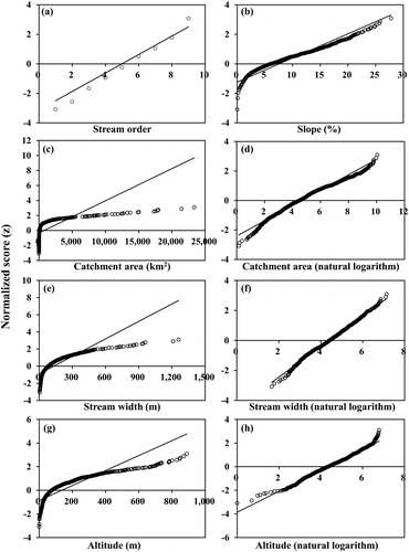
The variables used for PCA need to show normality (linear combination). As a result of the normality test for each physical variable, the raw values showed normality regarding stream order and slope. However, when they were transformed to $\ln (x+1),$ catchment area, stream width and altitude showed normality as well (Figure 2).

Figure 2. Normality test for each physical variable (a) stream order, (b) slope, (c, d) catchment area, (e, f) stream width and (g, h) altitude. Left figures of catchment area, stream width and altitude are raw values of each physical variable and right figures are the values converted to $\ln (x+1).$

PCA was conducted using the adjustment values ($A_1$) of each physical variable in order to identify the attributes of each physical variable (Figure 3). The total variance was 95.5% (Axis 1, 62.0%; Axis 2, 26.5%; Axis 3, 7.0%; Table 3). Axis one separated the five variables into stream size (stream order, catchment area and stream width) and gradient (altitude and slope). Stream order, catchment area and stream width showed significantly higher correlations with Axis 1. Among these, the stream width ($r=-0.923,\mathrm{ }p<0.01$) showed the highest correlation with Axis 1. Altitude and slope showed significantly higher correlations with Axis 2, with slope having a higher correlation ($r=0.743,\mathrm{ }p<0.01$). Axis three separated altitude from slope and presented the highest correlation with altitude ($r=-0.577,\mathrm{ }p<0.01$). However, the variance of Axis three was very low at 7%, which did not appear to be meaningful. The PCA and Pearson correlation analysis results allowed for stream order, catchment area and stream width to be integrated into stream size, while altitude and slope were integrated into the stream gradient variables.

Figure 3. PCA based on adjustment values ($A_1$) of each physical variable (a) Axis 1 versus Axis 2 and (b) Axis 2 versus Axis 3. The gray circles are 996 sampling sites and the arrow length is proportional to the relative importance of each physical variable.

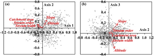
Table 3. Result of ordination by PCA of data on 996 sampling sites (a) axis summary of PCA and (b) Pearson correlation coefficients ($r$) for the three axes with five physical variables.

Variables	Axis 1	Axis 2	Axis 3
(a) Axis summary statistics of PCA results
Eigenvalue	0.115	0.049	0.013
% Variance explained	62.0	26.5	7.0
Cumulative % variance explained	62.0	88.5	95.5
(b) Correlation coefficient for five variables
Stream order	–0.901**	0.341**	0.000
Catchment area	–0.892**	0.398**	–0.001
Stream width	–0.923**	0.177**	–0.003
Altitude	0.521**	0.629**	–0.577**
Slope	0.608**	0.743**	0.279**

^** $p$ value < 0.01.

Distribution of FFG according to stream size and gradient

As stream order, catchment area and stream width increased, shredders and scrapers decreased and collectors increased, so the indicator value increased (Figure 4). Since there were only four sites of the first order, the first order and the second order were integrated. The mean indicator value in the stream order was low until the third order, then increased in the fourth order and thereafter, with inflection in both the sixth and seventh orders. The cumulative mean indicator value was also low until the third order, before increasing in the fourth order and above. However, the rate of increase was substantially decreased in the seventh order and above. Thus, the fourth and sixth intervals were determined to be the transitional zone at which the FFG composition changed, and the stream order was classified into low (first–third), transitional (fourth–sixth) and high order (seventh–ninth) streams, respectively.

Figure 4. Classification of (a–c) stream order, (d–f) catchment area and (g–i) stream width types based on indicator values of functional feeding groups. Left figures are relative composition ratio of each functional feeding group, middle figures are mean indicator values, and right figures are cumulative mean indicator values. CF: collector-filterer; CG: collector-gatherer; Pe: predator; Pi: plant-piercer; Sc: scraper; Sh: shredder.

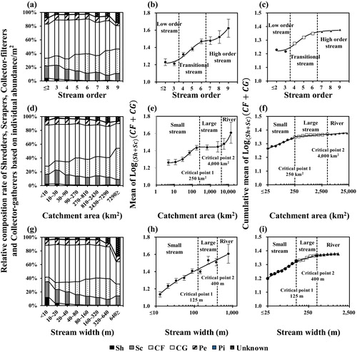
In the catchment area, the mean indicator value increased to 250 km², then remained at a certain level in the range of 250 to 4000 km² before increasing again at 4000 km² and above. The cumulative mean indicator value increased at all intervals. However, based on 250 km² there was a significant change in the rate of increase and was discontinuous at 250 and 4000 km². Thus, the catchment area was divided into small-scale and large-scale streams based on 250 km². The large-scale streams were further divided into large streams and rivers based on 4000 km². In other words, the catchment area was classified into small (small-scale) streams, large streams and rivers.

The mean indicator value in stream width increased almost linearly, indicating that the change in FFGs was influenced more by stream width compared to stream order or catchment area. The cumulative mean indicator value also continuously increased. However, the rate of increase was discontinuous at 125 and 400 m. Thus, the types of stream width were classified based on these discontinuous intervals. The stream width was divided into small (small-scale) streams and large-scale streams based on 125 m, and large-scale streams were further divided into large streams and rivers based on 400 m.

In contrast to the previous three variables, as altitude and slope increased, shredders and scrapers increased and collectors decreased, so the indicator values decreased (Figure 5). The mean indicator value decreased as the altitude increased, with an inflection at 450 m. The cumulative mean indicator value was discontinuous at 150 and 450 m. Thus, altitudes over 450 m were considered to be mountain streams for the aspect of FFGs and altitudes over 150 m and below 450 m were considered to be highland streams. Therefore, altitude was classified into mountain, highland and lowland streams based on 450 and 150 m.

Figure 5. Classification of (a–c) altitude and (d–f) slope types based on indicator values of functional feeding groups. Left figures are relative composition ratio of each functional feeding group, middle figures are mean indicator values and right figures are cumulative mean indicator values. CF: collector-filterer; CG: collector-gatherer; Pe: predator; Pi: plant-piercer; Sc: scraper; Sh: shredder.

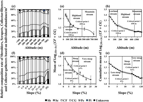
The mean indicator value decreased as slope increased, although the decrease was almost linear compared to altitude, indicating that the change in FFGs was influenced more by slope than by altitude. The cumulative mean indicator value continued to decrease, although the rate of decrease was discontinuous at the 8% and 14% intervals. The types of slope were divided based on discontinuous intervals. Thus, the slopes were classified into very steep streams, steep streams and less-steep streams based on 8% and 14%.

Influence of geology on benthic macroinvertebrate communities

CCA was conducted to analyze the effects of conductivity and pH, which represented geology, on the distribution of benthic macroinvertebrate communities (Figure 6). Axis one showed a high correlation with conductivity while Axis two showed a high correlation with pH (Table 4). However, based on the properties of biotic communities, the total variance up to Axis two that separately described the distribution of each site was only 12.8% (Axis 1, 10.5%; Axis 2, 2.3%). In addition, the Namhan River and the Bukhan River were not clearly distinguished by conductivity and pH. Indeed, when comparing the benthic macroinvertebrate communities of the Namhan River and the Bukhan River, there were differences in some taxa, but these differences were not large enough to judge to differ in taxa due to the influence of geology. In general, limestone zones are known to be more suitable for mollusks because they have higher concentrations of magnesium and calcium ions than granite zones (Carrie et al. 2015). In this study, however, the differences in taxa based on the difference between the two geology were found to be Heptageniidae, Plecoptera, and so forth, rather than mollusks. It is believed that the differences between taxa were due to habitat differences based on stream size and gradient rather than geology. This is not only the Republic of Korea’s nation size smaller than that of other countries but also because the limestone zone is a smaller part of the upper part of Namhan River, the geology itself does not seem to have a significant influence on the biotic communities compared to other physical variables.

Figure 6. CCA for the reference streams of Namhan River (NR: red squares) and Bukhan River (BR: blue circles) based on benthic macroinvertebrate assemblages with conductivity and pH. Arrow length is proportional to the relative importance of conductivity and pH.

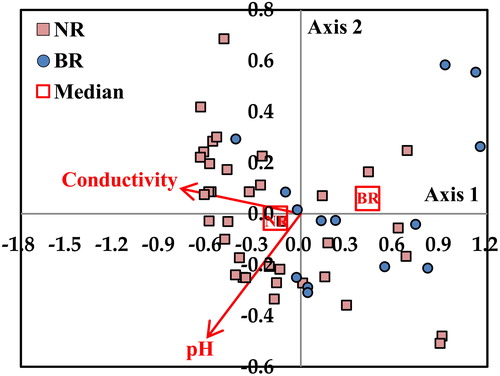
Table 4. Result of ordinations by CCA for reference streams of Namhan River and Bukhan River (a) axis summary of CCA and (b) Pearson correlation coefficients ($r$) for the two axes with two geological variables.

Variables	Axis 1	Axis 2
(a) Axis summary statistics of CCA results
Eigenvalue	0.190	0.042
% Variance explained	10.5	2.3
Cumulative % variance explained	10.5	12.8
Total inertia in the species data	1.807
(b) Correlation coefficient for five variables
Electric conductivity	–0.759**	0.100
pH	–0.602**	–0.517**

^** $p$ value < 0.01.

Stream classification

The streams were classified by combining the types of physical variables classified based on the indicator values of FFGs (Figures 4 and 5), excluding geology. Depending on the relationship between physical variables (Figures 2 and 3), it was necessary to select certain variables of stream size and gradient to classify streams in consideration of multicollinearity. According to the changes in the distribution of FFGs, it may be appropriate to classify streams using the stream width and slope, where the change of mean indicator values is almost linear, but these variables can be affected by natural and artificial disturbances. Thus, although the distribution of FFGs did not show a linear change compared to other variables, the stream was classified based on the catchment area and altitude with the least variability of variables from various disturbances.

First, with a focus on the stream size, the streams were divided into small- and large-scale streams, and small or large streams were further subdivided into the gradient. Streams with catchment areas under 250 km² were considered to be small-scale streams, while streams with catchment areas of 250 km² and above were considered to be large-scale streams. Large-scale streams were then further divided into large streams (catchment area of 250 to 4000 km²) and rivers (catchment area over 4000 km²). Based on altitude, small-scale streams were classified into Type 1 (over 450 m, mountain streams), Type 2 (150 to 450 m, highland small streams) or Type 3 (less than 150 m, lowland small streams), while large streams were classified into Type 4 (150 to 450 m, highland large streams) or Type 5 (less than 150 m, lowland large streams). The rivers were classified as Type 6 (Table 5).

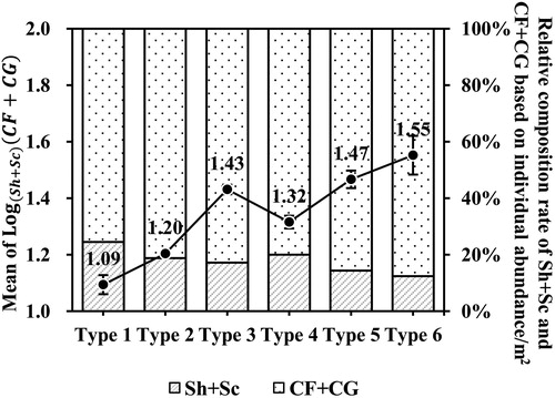
We reviewed mean changes in the indicator value and the relative individual abundance composition ratio of FFGs for stream classification criterion (Figure 7). As the gradient decreased with the same stream size, or when stream size increased with the same gradient, the indicator value was increased. In addition, the relative individual abundance composition ratio of shredders and scrapers decreased with Type 1 through Type 6, while that of collectors increased. Based on these results, according to the RCC, it appears that this proposed stream classification criterion could appropriately reflect changes in stream size and gradient in terms of FFGs.

Figure 7. Change in indicator value (black lines) and composition ratio of relative individual abundance (bar graph) of functional feeding groups (CF: collector-filterer; CG: collector-gatherer; Sc: scraper; Sh: shredder) according to stream types using catchment area and altitude.

We also reviewed whether the proposed classification criterion (Table 5) in the aspect of benthic macroinvertebrates assemblages, which are not FFGs, properly reflects assemblage changes or not (Figure 8). The taxa richness, percentage of Ephemeroptera, Plecoptera, Trichoptera (EPT) richness, percentage of EPT abundance, diversity index (Shannon and Weaver 1949), and benthic macroinvertebrate index (BMI; Kong et al. 2018) decreased with increasing stream types. BMI is a revised version of the saprobic index (Zelinka and Marvan 1961), and this index has been used for biotic water quality assessment based on benthic macroinvertebrates in the Republic of Korea. Changes in biotic assemblages depending on stream type were apparent, but unlike other biotic indices, taxa abundance increased as stream types increased (Type 1 to Type 6); however, it was largely decreased in Type 6 (rivers). Indicator value of FFGs tended to be increased according to stream types from Type 1 to Type 6, whereas the biotic assemblages except individual abundance tended to decrease, showing inverse relationships with each other. This means that FFGs can represent specific biotic index (e.g. EPT) and can be used as an index for biotic assessment of lotic aquatic ecosystems.

Figure 8. Changes in indices of benthic macroinvertebrate assemblage (a) taxa richness, (b) taxa abundance, (c) EPT richness (%), (d) EPT abundance (%), (e) Shannon diversity index and (f) BMI according to the stream types (1 to 6). The boxes represent the 25th and 75th percentiles and the whiskers indicate the 5th and 95th percentiles with standard deviations (error bar). The horizontal dotted lines and solid lines in each box represent the mean and median, respectively.

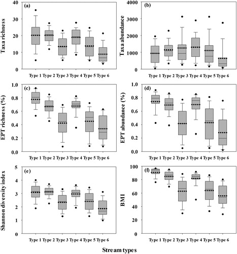
Table 5. Stream classification criterion using catchment area and altitude.

First division			Second division
Catchment area (km^2)	Division		Altitude (m)	Subdivision (stream type)
<250 (714)	Small-scale (714)		450< (56)	Type 1 (56)	Mountain streams
			150 – 450 (184)	Type 2 (184)	Highland small streams
			<150 (474)	Type 3 (474)	Lowland small streams
250–4000 (231)	Large-scale (282)	Large streams (231)	150 – 450 (52)	Type 4 (52)	Highland large streams
			<150 (179)	Type 5 (179)	Lowland large streams
<4000 (51)		Rivers (51)	– (51)	Type 6 (51)	Rivers

Numbers in parentheses indicate numbers of sites.

Discussion

Attributes of physical variables

Since stream order, catchment area and stream width are quantitative indicators of stream scale, these are the variables that represent stream size (Olivero and Anderson 2008; Kim et al. 2017). Thus, these variables had high and significant correlations (Table 2) and were found to be located on the same PCA plot (Figure 3). Altitude and slope have a commonality in that they can be approached from a vertical perspective of the stream, regardless of stream size. However, these two variables have strictly different attributes. As altitude has a strong relationship with water temperature, a change in altitude can substantially influence the distribution of biota (cold water or warm water species) by changing the water temperature (Jacobsen et al. 1997). On the other hand, since slope has a strong relationship with flow velocity and streambed composition, a change in slope can substantially influence the distribution of biota (lotic and lentic or clinging and burrowing species) by changing the habitat type (e.g. riffle, run and pool; Olivero and Anderson 2008). Nevertheless, altitude and slope were shown to be highly correlated with each other (Table 2) and located in the same PCA plot (Figure 3). Thus, both variables were considered as the stream gradient. Geology is only divided based on the type of material. This variable can influence the distribution of biota, mainly by affecting the water chemical variables (e.g. hardness and buffer action) of streams (Olivero and Anderson 2008; Carrie et al. 2015). Thus, geology itself was considered as the independent variable.

Distribution characteristics of biota according to physical variables

Benthic macroinvertebrate FFGs were classified based on the food sources and food acquisition behaviors instead of simply following the morphological classification (Cummins and Klug 1979). Biotic function-based classification is an effective means to distinguish each species ecologically (Merritt and Cummins 1996), ultimately contributing to the development of biotic indices that can identify the function of stream ecosystems (Kerans and Karr 1994; Barbour et al. 1996). In general, it is known that the distributions of shredders, scrapers and collectors among the FFGs are influenced by the longitudinal gradient of streams (Allan and Castillo 2007), and FFGs were also used as components of the benthic macroinvertebrate multimetric index (Jun et al. 2012; USEPA 2013; Sirisinthuwanich et al. 2016). Thus, we set a biotic indicator of FFGs using shredders, scrapers and collectors, as opposed to simply using the distribution of each FFG. Based on the indicator, we analyzed the distribution patterns of FFGs according to stream size and gradient. When setting up the indicators for FFGs, the individual abundance of each group was used and the ratio of downstream indicator groups to upstream indicator groups was set instead of simply analyzing the distribution of each FFG. As their main food sources, shredders use CPOM, while scrapers use algae attached to the surface of coarse bedrock. Accordingly, scrapers mainly contain many taxa inhabiting the coarse substrates, which are predominantly upstream rather than downstream. In addition, in this study, not only the individual abundance of shredders was very small, but the change in scrapers tended to be similar to shredders that the composition ratio decreased as the stream size increased (Figure 4). For this reason, both shredders and scrapers were considered to be the functional groups that represent upstream watersheds. On the other hand, collectors (filterers and gatherers) use FPOM as their main food source. In addition, due to the fact that the composition ratio increased with stream size increased, the collectors were considered to be the functional groups that represent downstream watersheds (Minshall et al. 1983; Oliveira and Nessimian 2010).

Intervals where the rate of increase or decrease of the mean and cumulative mean indicator value presented changes were considered to be the intervals in which the distribution of FFGs changed. Since stream order, catchment area and stream width were all variables that represent the stream size, the indicator values increased with stream size, but the increase patterns were different for each variable. Among the variables of stream size, stream width was a variable whose mean indicator value changed in an almost linear manner. This possess a greater influence on the distribution of FFGs compared to stream order and catchment area (Figure 4). This is because stream order and catchment area were potential indicators representing stream size, while stream width was an actual measurement reflecting physical properties. In terms of stream order, the mean indicator value showed an inflection point between the sixth and seventh orders, but it presented a tendency to increase continuously. On the other hand, the mean indicator value maintained a certain value at the 250 to 4000 km² interval in the catchment area. It is considered that the mean indicator value was shown at a certain level in the catchment area because this study only investigated the riffles of the streams. The availability of food is a factor clearly affecting the occurrence of species (Oliveira and Nessimian 2010), and species are common in habitats where their food is readily available (Hynes 1970). Typically, riparian vegetation, an allochthonous feeding resource, influences the distribution of shredders as a major source of energy in the upstream (Allan and Castillo 2007). The water flow influences the amount of available food, promoting the release and/or remotion of nutrients and substrates with the capacity to retain most of the organic matter available, providing shelter and abundant food (Oliveira and Nessimian 2010). Collector-filterers select habitats with fast-flowing water that provides more organic matter in a shorter period of time (Buss et al. 2002; Uwadiae 2010), and they appear to be adapted to this microhabitat, considering that they use specialized mouthparts to filter fine organic matter in suspension (Cummins et al. 2005; Baptista et al. 2006). Scrapers are mainly influenced by substrates that are used as shelter and including periphyton, used as a main food source (Bhawsar et al. 2015). Thus, the presence of scrapers and collector-filterers was associated with riffle habitats, which include fast water flow and coarse substrates, and these organisms were shown to have higher abundance in the riffle area (Oliveira and Nessimian 2010; Bhawsar et al. 2015). Based on this concept, it is believed that the interval in which the mean indicator value remained at a certain value in the catchment area was attributable to the presence of scrapers and collector-filterers in a similar proportion in terms of individual abundance at riffle habitats. Among the variables including the gradient, slope had a greater influence on the distribution of FFGs than altitude by changing the mean indicator value in an almost linear fashion (Figure 5). The slope has a direct effect on the microhabitats inhabited by the organisms, and the slope is considered to have a larger influence than altitude.

Since the geology is classified according to the rock material irrespective of the longitudinal gradient of the stream, and its influence was confirmed using biotic communities. Geology was analyzed in terms of its influence on benthic macroinvertebrate communities using conductivity and pH after selecting reference streams within the granite and limestone zones. However, there was no distinct difference between biotic communities (Figure 6). Sites with different geology were not clearly separated in reference streams, where various environmental variables were in a homogeneous condition in a suitable range for inhabitation by benthic macroinvertebrates. This finding suggested that, in the simple geological distribution according to granite and limestone zones, there were no distinct differences between geology and benthic macroinvertebrate communities, indicating that geology had little influence on the distribution of biotic communities.

Stream classification criterion and biotic assemblages

Physical stream variables are very diverse (e.g. stream order, catchment area, stream width, altitude, slope, flow velocity, water depth, geology and streambed substrate size), and the stream classification criteria can also vary depending on which variables are used. Davis (1899) was the first to classify stream types when distinguishing geographical features such as valley floors, river branches and meanders according to the time of stream formation. Since then, a number of stream classification criteria have been proposed based on the channel shape, stability and slope (Leopold and Wolman 1957; Rosgen 1994). In the typical classification process described by Rosgen (1994), streams can be classified based on geomorphic (slope and sinuosity) properties and subdivided according to morphological properties (width/depth ratio, dominant streambed particle size and entrenchment). Rosgen (1994) developed a universal classification criterion with which to classify stream types more systematically and thoroughly by applying physical variables as quantitative values. However, since this classification can vary in type depending on the stream reach, multiple types may appear repeatedly in a single stream. In addition, it is difficult to reflect the unique functions and properties of streams that only appear in upstream or downstream stretches. Moreover, different stream types may occur in the same reach due to natural or artificial disturbances. If the purpose of stream classification is to develop a biotic survey and assessment methods in consideration of the functions and properties of streams and to understand the characteristics of each type in future studies examining restoration and conservation, then stream types classified based on specific typology should be classified into the same type according to the same typology after a long time (WFD 2000). Thus, streams have to be classified using physical variables with small variability from disturbances. In the United States, streams or habitats are classified using a number of variables, such as stream order, catchment area, slope and geology, where the variable variability is small (Walsh et al. 2007; Olivero and Anderson 2008; Ohio EPA 2015; USEPA 2018). In the European Union, streams are also classified in each country in terms of catchment area, altitude and geology that are physical variables with low variability according to WFD’s (2000) recommendations (AQEM Consortium 2002; Ferréol et al. 2005; Arle et al. 2014). Thus, stream order, catchment area, stream width, altitude, slope and geology are appropriate physical variables for classifying streams in the Republic of Korea.

After classifying each physical variable into higher groups based on the analysis results, some variables influencing the benthic macroinvertebrate assemblages were selected for each group to classify streams considering multicollinearity. Thus, five physical variables excluding geology were considered for stream classification, and these were divided into two attribute groups (size and gradient; Table 2 and Figure 3, respectively). If these variables each had different physical stream property, it would be appropriate to classify streams using all variables. However, the classification process may be complicated if variables with the same properties are used repeatedly, and certain variables may be unnecessary. Thus, streams were classified by selecting only some stream size and gradient variables. Stream width had an almost linear relationship with changes in mean indicator value among the variables of stream size, and this was also the case with the slope among the variables of gradient. Based on these results, it may be appropriate to classify streams using the stream width and slope, but these are variables that can be changed by natural or artificial disturbances, so it may be difficult to consider as consistent variables. Stream width is highly fluctuating variable because there are many disturbances. Geographically, the Republic of Korea is located on the eastern side of the mid-latitude continent. It has four distinct seasons because it is affected by both continental and oceanic influences (Lee et al. 2005). As the amount of precipitation in the summer monsoon period accounts for approximately 60% ∼ 70% of the annual precipitation, severe flooding events are frequent (Lee et al. 2011; Jun et al. 2016). On the other hand, in seasons other than summer, the water flow is reduced due to the dry seasons. For this reason, the coefficient of river regime of Republic Korean streams is higher than that of streams in other countries (Lee et al. 2014). Natural disasters, such as flooding events, cause erosion of natural levee causing stream width changes. In addition, to stabilize unstable coefficient of river regime, the natural levee is modified into artificial banks (Lee et al. 2014) and this control changes the stream width. Further, stream width depends on how the measurement interval length is measured. Slope could be also changed due to natural changes caused by erosion and deposition as well as artificial streambed modification and channelization. In addition, stream order may vary depending on the map scale. On the other hand, catchment area and altitude are variables that can potentially determine the physical properties of streams; although they are not direct indicators of topographic properties of streams, they are useful in that they are constants unchanged by disturbances. Therefore, we suggested the classification criterion using catchment area and altitude in accordance with the WFD’s (2000) recommendations.

Furthermore, the mean indicator value of FFGs and biotic indices based on benthic macroinvertebrate assemblages after classifying stream types were studied (Figures 7 and 8). The mean indicator value and relative individual abundance composition ratio of collectors (filterers and gatherers) were increased, but the relative individual abundance composition ratio of shredders and scrapers was decreased as the stream types increased (Type 1 to Type 6). In addition, the biotic indices except for taxa abundance were decreased as the stream types were increased. At this time, the indicator value and biotic indices were changed in a more linear fashion when they were located in the order of Type 1 ∼ 2 (mountain streams to highland small streams), Type 4 (highland large streams), Type 3 (lowland small streams) and Type 5 ∼ 6 (lowland large streams to rivers). This is because the distribution of benthic macroinvertebrates is more influenced by altitude (stream gradient) than catchment area (stream size; Sandin 2003; Jun et al. 2016). It is known that altitude has previously been proposed as a potential variable to determine various environments (e.g. water temperature, hydrology, water quality and habitat), which can influence the distribution of benthic macroinvertebrates (Beauchard et al. 2003; Li et al. 2012). The mean values of taxa abundance were increased as the stream types increased, but then largely decreased in Type 6 (rivers). This indicated that the characteristics of physical habitat environment, based on the interval with a catchment area of over 4000 km², are shifting from streams to rivers, which are a somewhat unfavorable environment for benthic macroinvertebrate habitat. These environments can form monotonous habitats due to their deep water depth, fine substrates and slow water flow, thereby reducing biodiversity and causing overall individual abundance dwindling (Carter and Fend 2001). These results suggest that the proposed classification criterion was able to adequately reflect changes in physical stream variables in the biotic aspect according to the RCC. The percentage of EPT richness and abundance, diversity index and BMI of lowland streams (Types 3, 5 and 6) had a larger range of first and third quartiles than the highland streams (Types 1, 2 and 4). This could be attributable to the relatively high rates of disturbed streams passing through lowland cities (Jun et al. 2016).

Our study examined the influences of stream size and gradient on the distribution of benthic macroinvertebrate FFG, and the results were found to be similar to those in the RCC (Vannote et al. 1980). The results of this study are expected to elucidate the overall process-level lotic ecosystem of Korean streams by analyzing the changes in the distribution of FFG at the national scale. However, in order to understand the important environmental variables that significantly affect the distribution of biota, it is necessary to further study at the level of microhabitats and using various variables. These studies are expected to be used as basic information for habitat restoration research for biodiversity and the development of indices for the biotic assessment of streams.

Disclosure statement

No potential conflict of interest was reported by the authors.

Additional information

Funding

This study was supported by the Kyonggi University Research Grant 2018 under Grant 2018-028.

Notes on contributors

Jeong-Ki Min

Jeong-Ki Min is currently a PhD student at Kyonggi University, Republic of Korea. He is majoring aquatic ecology, especially benthic macroinvertebrates.

Ye-Ji Kim

Ye-Ji Kim is currently a PhD student at Kyonggi University, Republic of Korea. She is majoring aquatic ecology, especially benthic macroinvertebrates.

Dong-Soo Kong

Dong-Soo Kong was the chief of Han River Environment Research Center at the National Institute of Environmental Research. He is currently a professor of Kyonggi University, Republic of Korea and majoring water quality management and freshwater ecology related to aquatic organisms such as benthic macroinvertebrates, fishes, and algae.

Appendix 1. Functional feeding groups in response to the benthic macroinvertebrates that appeared in this study

 

Table

Taxa	FFG	Taxa	FFG
Platyhelminthes		Viviparidae	Sc
Planariidae	Pe	Annelida
Nematomorpha		Anisogammaridae	CG
Gordiidae	Unknown	Asellidae	Unknown
Mollusca		Erpobdellidae	Pe
Ampullariidae	Sc	Gammaridae	CG
Assimineidae	Sc	Glossiphoniidae	Pe
Bithyniidae	Sc	Hirudinidae	Pe
Corbulidae	CF	Lumbricidae	CG
Cyrenidae	CF	Naididae	Unknown
Laternulidae	CF	Nereididae	CG
Lymnaeidae	Sc	Tubificidae	CG
Mytilida	CF	Arthropoda
Neritidae	Sc	Atyidae	CG
Physidae	Sc	Cambaroididae	Pe
Planorbidae	Sc	Grapsidae	Pe
Pleuroceridae	Sc	Palaemonidae	Pe
Sphaeriidae	CF	Sergestidae	CG
Stenothyridae	Sc	Sesarmidae	Pe
Succineidae	Sc	Varunidae	Pe
Trochidae	Sc	Ephemeroptera
Unionida	CF	Ameletidae	Sc
Baetidae	CG	Capniidae	Sh
Caenidae	CG	Chloroperlidae	Pe
Ephemerellidae	CG, Sc	Leuctridae	Sh
Ephemeridae	CG	Nemouridae	Sh
Heptageniidae	CG, Sc	Peltoperlidae	Sh
Isonychiidae	CF	Perlidae	Pe
Leptophlebiidae	CG	Perlodidae	Pe
Neoephemeridae	CG	Pteronarcidae	Sh
Polymitarcyidae	CG	Scopuridae	Sh
Potamanthidae	CG	Taeniopterygidae	Unknown
Siphlonuridae	CG	Hemiptera
Odonata		Aphelocheiridae	Pe
Aeshnidae	Pe	Belostomatidae	Pe
Calopterygidae	Pe	Corixidae	Pe, Pi
Coenagrionidae	Pe	Gerridae	Pe
Cordulegastridae	Pe	Mesoveliidae	Pe
Corduliidae	Pe	Nepidae	Pe
Gomphidae	Pe	Notonectidae	Pe
Lestidae	Pe	Pleidae	Pe
Libellulidae	Pe	Veliidae	Pe
Macromiidae	Pe	Megaloptera
Platycnemididae	Pe	Corydalidae	Pe
Plecoptera		Sialidae	Pe
Coleoptera		Empididae	Pe
Chrysomelidae	Sh	Ephydridae	CG
Dytiscidae	Pe	Limoniidae	Pe
Elmidae	CG, Sc	Muscidae	Pe
Gyrinidae	Pe	Psychodidae	CG
Haliplidae	Pi	Sciomyzidae	Pe
Hydrophilidae	CG	Simuliidae	CF
Lampyridae	Pe	Stratiomyidae	CG
Noteridae	Pe	Syrphidae	CG
Psephenidae	Sc	Tabanidae	Pe
Scirtidae	Sc	Tipulidae	CG, Pe, Sh
Neuroptera		Trichoptera
Sisyridae	Pe	Apataniidae	Sc
Diptera		Brachycentridae	Sh
Athericidae	Pe	Calamoceratidae	Sh
Blephariceridae	Sc	Ecnomidae	CF
Ceratopogonidae	Pe	Glossosomatidae	Sc
Chaoboridae	Pe	Goeridae	Sc
Chironomidae	CG	Hydrobiosidae	Pe
Culicidae	CG	Hydropsychidae	CF
Deuterophlebiidae	Sc	Hydroptilidae	Pi
Dixidae	CG	Lepidostomatidae	Sh
Dolichopodidae	Pe	Leptoceridae	CG
Limnephilidae	Sh	Polycentropodidae	CF
Molannidae	Sc	Psychomyiidae	CG
Odontoceridae	Sc	Rhyacophilidae	Pe
Philopotamidae	CF	Sericostomatidae	Sh
Phryganeidae	Sh	Stenopsychidae	CF
Phryganopsychidae	Unknown	Uenoidae	Sc

CF: collector-filterer; CG: collector-gatherer; FFG: functional feeding group; Pe: predator; Pi: plant-piercer; Sc: scraper; Sh: shredder.

References

- Allan JD, Castillo MM. 2007. Stream ecology: structure and function of running waters. Dordrecht: Springer Science & Business Media.
- AQEM Consortium. 2002. Manual for the application of the AQEM system. A comprehensive method to assess European streams using benthic macroinvertebrates, developed for the purpose of the water framework directive, version, 1. Germany: University Duisburg-Essen. Contract No: EVK1-CT1999-00027, EU Projects. European Union.
- Arle J, Blondzik K, Claussen U, Duffek A, Grimm S, Hilliges F, Hoffmann A, Leujak W, Mohaupt V, Naumann S, et al. 2014. Environmental policy, water resources management in Germany. Part 2. Water quality, federal ministry of environment, nature conservation, building and nuclear safety, 53048 Bonn. Bonn: Federal Ministry for the Environment, Nature Conservation, Construction and Nuclear Safety.
- Bae YJ, Won DH, Lee WJ, Seung HW. 2003. Development of environment assessment technique and biodiversity management system and their application to stream ecosystems in Korea. Korean J Environ Biol. 21(3):223–233.
- Baptista DF, Buss DF, Dias LG, Nessimian JL, Da Silva ER, De Moraes Neto AHA, de Carvalho SN, De Oliveira MA, Andrade LR. 2006. Functional feeding groups of Brazilian Ephemeroptera nymphs: ultrastructure of mouthparts. Ann Limnol - Int J Lim. 42:87–96.
- Barbour MT, Gerritsen J, Griffith GE, Frydenborg R, McCarron E, White JS, Bastian ML. 1996. A framework for biological criteria for Florida streams using benthic macroinvertebrates. J North Am Benthol Soc. 15(2):185–211.
- Barman B, Gupta S. 2015. Spatial distribution and functional feeding groups of aquatic insects in a stream of Chakrashila Wildlife Sanctuary. Assam, India. Knowl Manag Aquat Ecosyst. 416:37.
- Beauchard O, Gagneur J, Brosse S. 2003. Macroinvertebrate richness patterns in North African streams. J Biogeogr. 30(12):1821–1833.
- Bhawsar A, Bhat MA, Vyas V. 2015. Distribution and composition of macroinvertebrates functional feeding groups with reference to catchment area in Barna Sub-Basin of Narmada River Basin. IJSRES. 3(11):385–393.
- Brasil LS, Juen L, Batista JD, Pavan MG, Cabette H. 2014. Longitudinal distribution of the functional feeding groups of aquatic insects in streams of the Brazilian Cerrado Savanna. Neotrop Entomol. 43(5):421–428.
- Buss DF, Baptista DF, Silveira MP, Nessimian JL, Dorvillé L. 2002. Influence of water chemistry and environmental degradation on macroinvertebrate assemblages in a river basin in South-East Brazil. Hydrobiologia. 481(1/3):125–136.
- Carrie R, Dobson M, Barlow J. 2015. The influence of geology and season on macroinvertebrates in Belizean streams: implications for tropical bioassessment. Freshw Sci. 34(2):648–662.
- Carter JL, Fend SV. 2001. Inter-annual changes in the benthic community structure of riffles and pools in reaches of contrasting gradient. Hydrobiologia. 459(1/3):187–200.
- Cummins KW. 1973. Trophic relations of aquatic insects. Annu Rev Entomol. 18(1):183–206.
- Cummins KW. 1974. Structure and function of stream ecosystems. BioScience. 24(11):631–641.
- Cummins KW, Klug MJ. 1979. Feeding ecology of stream invertebrates. Annu Rev Ecol Syst. 10(1):147–172.
- Cummins KW, Merritt RW, Andrade PC. 2005. The use of invertebrate functional groups to characterize ecosystem attributes in selected streams and rivers in south Brazil. Stud Neotrop Fauna Environ. 40(1):69–89.
- Davis WM. 1899. The geographical cycle. Geogr J. 14(5):481–504.
- Fenoglio S, Badino G, Bona F. 2002. Benthic macroinvertebrate communities as indicators of river environment quality: an experience in Nicaragua. Rev Biol Trop. 50(3–4):1125–1131.
- Ferréol M, Dohet A, Cauchie H-M, Hoffmann L. 2005. A top-down approach for the development of a stream typology based on abiotic variables. Hydrobiologia. 551(1):193–208.
- Fierro P, Bertrán C, Mercado M, Peña-Cortés F, Tapia J, Hauenstein E, Caputo L, Vargas-Chacoff L. 2015. Landscape composition as a determinant of diversity and functional feeding groups of aquatic macroinvertebrates in southern rivers of the Araucanía, Chile. Lat Am J Aquat Res. 43(1):186–200.
- Fu L, Jiang Y, Ding J, Liu Q, Peng QZ, Kang MY. 2016. Impacts of land use and environmental factors on macroinvertebrate functional feeding groups in the Dongjiang River basin, southeast China. J Freshw Ecol. 31(1):21–35.
- George ADI, Abowei JFN, Alfred-Ockiya JF. 2010. The distribution, abundance and seasonality of benthic macro invertebrate in Okpoka creek sediments, Niger Delta, Nigeria. Res J Appl Sci Eng Technol. 2(1):11–18.
- Glaz P, Sirois P, Nozais C. 2012. Determination of food sources for benthic invertebrates and brook trout Salvelinus fontinalis in Canadian Boreal Shield lakes using stable isotope analysis. Aquat Biol. 17(2):107–117.
- Heino J, Parviainen J, Paavola R, Jehle M, Louhi P, Muotka T. 2005. Characterizing macroinvertebrate assemblage structure in relation to stream size and tributary position. Hydrobiologia. 539(1):121–130.
- Hwang S-J, Kim N-Y, Yoon SA, Kim B-H, Park MH, You K-A, Lee HY, Kim HS, Kim YJ, Lee J, Lee OM, et al. 2011. Distribution of benthic diatoms in Korean rivers and streams in relation to environmental variables. Ann Limnol Int J Lim. 47(S1):S15–S33.
- Hynes HBN. 1970. The ecology of running waters. Vol. 555. Liverpool: Liverpool University Press.
- Jacobsen D, Schultz R, Encalada A. 1997. Structure and diversity of stream invertebrate assemblages: the influence of temperature with altitude and latitude. Freshw Biol. 38(2):247–261.
- Jiang X-M, Xiong J, Qiu J-W, Wu J-M, Wang J-W, Xie Z-C. 2010. Structure of macroinvertebrate communities in relation to environmental variables in a subtropical Asian river system. Int Rev Hydrobiol. 95(1):42–57.
- Jun Y-C, Kim N-Y, Kim S-H, Park Y-S, Kong D-S, Hwang S-J. 2016. Spatial distribution of benthic macroinvertebrate assemblages in relation to environmental variables in Korean Nationwide streams. Water. 8(1):27.
- Jun Y-C, Won D-H, Lee S-H, Kong D-S, Hwang S-J. 2012. A multimetric benthic macroinvertebrate index for the assessment of stream biotic integrity in Korea. Int J Environ Res Public Health. 9(10):3599–3628.
- Kerans BL, Karr JR. 1994. A benthic Index of Biotic Integrity (B-IBI) for rivers of the Tennessee Valley. Ecol Appl. 4(4):768–785.
- Kim D-H, Chon T-S, Kwak G-S, Lee S-B, Park Y-S. 2016. Effects of land use types on community structure patterns of benthic macroinvertebrates in streams of urban areas in the South of the Korea Peninsula. Water. 8(5):187.
- Kim J-Y, Kim P-J, Hwang S-J, Lee J-K, Lee S-W, Park C-H, Moon J-S, Kong D-S. 2017. Korean stream types based on benthic macroinvertebrate communities according to stream size and altitude. J Freshw Ecol. 32(1):741–759.
- Kim KH, Shim ES. 2001. Geochemical characteristics and origin of dissolved ions in the Han River water. Econ Environ Geol. 34(6):539–553.
- Kong DS, Son SH, Hwang SJ, Won DH, Kim MC, Park JH, Jeon TS, Le JE, Kim JH, Kim JS, et al. 2018. Development of Benthic Macroinvertebrates Index (BMI) for biological assessment on stream environment. J Korean Soc Water Environ. 34(2):183–201.
- Lee K-S, Keun RJ, Jin AS. 2014. Change of regime coefficient due to dredging and dam construction. J KEDS. 40(1):30–38.
- Lee SH, Heo IH, Lee KM, Kwon WT. 2005. Classification of local climatic regions in Korea. Korean Meteorol Soc. 41(6):983–995.
- Lee S-W, Hwang S-J, Lee J-K, Jung D-I, Park Y-J, Kim J-T. 2011. Overview and application of the National aquatic ecological monitoring program (NAEMP) in Korea. Ann Limnol Int J Lim. 47(S1):S3–S14.
- Leopold LB, Wolman MG. 1957. River channel patterns: braided, meandering, and straight. Geological Survey Professional Paper. Washington (DC): US Government Printing Office.
- Li F, Chung N, Bae M-J, Kwon Y-S, Park Y-S. 2012. Relationships between stream macroinvertebrates and environmental variables at multiple spatial scales. Freshw Biol. 57(10):2107–2124.
- Merritt RW, Cummins KW. 1996. An introduction to the aquatic insects of North America. 3rd ed. Iowa: Kendall/Hunt Publishing Company.
- Merz JE, Ochikubo C. 2005. Effects of gravel augmentation on macroinvertebrate assemblages in a regulated California river. River Res Appl. 21(1):61–74.
- Ministry of Environment [ME]. 2011. Ecological river restoration techniques guideline. Technical specification. Sejong Metropolitan Autonomous City, Republic of Korea: The Ministry of Environment.
- ME. 2017. Study on the selection and application of the reference streams in the stream/river ecosystem (II). Sejong Metropolitan Autonomous City, Republic of Korea: Ministry of Environment.
- ME and NIER. 2013. Survey and evaluation of aquatic ecosystem health in Korea (V). Incheon Metropolitan City, Republic of Korea: The National Institute of Environmental Research.
- Minshall GW, Petersen RC, Cummins KW, Bott TL, Sedell JR, Cushing CE, Vannote RL. 1983. Interbiome comparison of stream ecosystem dynamics. Ecol Monogr. 53(1):1–25.
- NIER. 2015. Korean Reach File (KRF) of water environment information system. [accessed 2018 November] http://water.nier.go.kr/publicFront/gisInfo/gisKrf.jsp?menuIdx=5_3#rivernetwork_contents02.
- Nelson SM, Lieberman DM. 2002. The influence of flow and other environmental factors on benthic invertebrates in the Sacramento river, USA. Hydrobiologia. 489(1/3):117–129.
- Ohio EPA. 2015. Biological criteria for the protection of aquatic life. State of Ohio, USA: Ohio Environmental Protection Agency, Division of Water Ecological Assessment Section. Biocriteria Manual Volume III. Revised June 2015.
- Oliveira A, Nessimian JL. 2010. Spatial distribution and functional feeding groups of aquatic insect communities in Serra da Bocaina streams, Southeastern Brazil. Acta Limnol Bras. 22(4):424–441.
- Olivero AP, Anderson MG. 2008. Northeast aquatic habitat classification system. Arlington County (VA): The Nature Conservancy, Eastern Regional Office.
- Parsons M, Thoms M, Norris R. 2001. Australian river assessment system: AusRivAS physical assessment protocol. Monitoring River Health Initiative Technical Report. Report Number 22. Canberra, Australia: Environmental Australia.
- Príncipe RE, Gualdoni CM, Raffani GB, Corigliano MC. 2010. Spatial-temporal patterns of functional feeding groups in mountain streams of Córdoba, Argentina. Ecol Austral. 20:257–268.
- Ro TH, Chun DJ. 2004. Functional feeding group gatergorization of Korean immature aquatic insects and community stability analysis. Korean J Limnol. 37(2):137–148.
- Rosenberg DM, Danks H, Lehmkuhl DM. 1986. Importance of insects in environmental impact assessment. Environ Manage. 10(6):773–783.
- Rosgen DL. 1994. A classification of natural rivers. Catena. 22(3):169–199.
- Ryu JS, Chang HW, Lee KS. 2008. Hydrogeochemistry and isotope geochemistry of the Han River system: a summary. J Geol Soc Korea. 44(4):467–477.
- Sandin L. 2003. Benthic macroinvertebrates in Swedish streams: community structure, taxon richness, and environmental relations. Ecography. 26(3):269–282.
- Shannon CE, Weaver W. 1949. The mathematical theory of communication. Urbana (IL): The Board of Trustees of the University of Illinois Press.
- Sirisinthuwanich K, Sangpradub N, Hanjavanit C. 2016. Development of biotic index to assess the Phong and Cheon rivers’ healths based on benthic macroinvertebrates in Northeastern Thailand. AACL Bioflux. 9(3):680–694.
- Smith MJ, Kay WR, Edward DHD, Papas PJ, Richardson STJ, Simpson JC, Pinder AM, Cale DJ, Horwitz PHJ, Davis JA, et al. 1999. AusRivAS: using macroinvertebrates to assess ecological condition of rivers in Western Australia. Freshw Biol. 41(2):269–282.
- Strahler AN. 1957. Quantitative analysis of watershed geomorphology. Trans AGU. 38(6):913–920.
- Ter Braak C. 1986. Canonical correspondence analysis: a new eigenvector technique for multivariate direct gradient analysis. Ecology. 67(5):1167–1179.
- United States Environmental Protection Agency, Office of Research and Development [USEPA]. 2013. National rivers and streams assessment 2008–2009. Washington (DC): USEPA.
- USEPA. 2018. National rivers and streams assessment 2018/19: site evaluation guidelines. Washington (DC): USEPA.
- Uwadiae RE. 2010. Macroinvertebrates functional feeding groups as indices of biological assessment in a tropical aquatic ecosystem: implications for ecosystem functions. N Y Sci J. 3(8):6–15.
- Vannote RL, Minshall GW, Cummins KW, Sedell JR, Cushing CE. 1980. The river continuum concept. Can J Fish Aquat Sci. 37(1):130–137.
- Wallace JB, Webster JR. 1996. The role of macroinvertebrates in stream ecosystem function. Annu Rev Entomol. 41(1):115–139.
- Walsh MC, Deeds J, Nightingale B. 2007. Classifying lotic systems for conservation: methods and results of the Pennsylvania aquatic community classification. Pittsburgh (PA): Pennsylvania Natural Heritage Program, Western Pennsylvania Conservancy.
- WFD. 2000. E.U. Directive 2000/60/EC of the European parliament and of the council establishing a framework for the community action in the field of water policy. Brussels: The European Parliament and the Council of the European Union.
- Yun CW, Moon HS. 2009. Classification of forest vegetation type and environmental properties in limestone area of Korea. J Agric Life Sci. 43(2):1–8.
- Zelinka M, Marvan P. 1961. Zur präazisierung der biologischen klassifikation der reinheid fliessender gewäasser. Arch. Hydrobiol. 57(3):389–407.