Using soil micromorphology to assess the reliability of radiocarbon and OSL dating of fluvial deposits

ABSTRACT

Two sediment profiles exposed along the floodplain of the Tennessee River provide an excellent opportunity to compare radiocarbon and optically stimulated luminescence dating of fluvial sediments, and to use soil micromorphology as a tool to assess the reliability of these dating methods. The profiles occur as vertical stacks of floodplain soils, buried soils, and fluvial deposits, with the sediments of both profiles indicating an alluvial origin, but with different degrees of soil development. Micromorphological analysis showed pedogenic clay coatings are common in both profiles. These pedofeatures provide evidence of relative age of the deposits, because layered, well-developed, thick clay coatings generally take thousands of years to form. Radiocarbon results indicate that the profiles span from the late early Holocene to late Holocene. OSL dating indicates that one profile is relatively recent (<600 yrs. B.P.) while the other is of late middle Holocene age (3.2 ka B.P. to 5.3 ka B.P.). Clay coatings support the results from OSL because the relatively recent profile has very thin coatings, in contrast with thick, well-developed clay coatings in the older profile. Some of the radiocarbon ages appear to be too old owing to redeposition, but other dates are consistent with soil development and micromorphology.

KEYWORDS:

• Fluvial sediments
• radiocarbon dating
• Optically stimulated luminescence
• soil micromorphology
• Tennessee river

Introduction

Fluvial deposits, landforms, and floodplain soils and paleosols are important archives of information for reconstructing paleoclimate (Demko et al., 2004; Driese et al., 2005, 2008; Hatano & Yoshida, 2017; Smith et al., 2018), paleoenvironments (Chumbley et al., 1990; He et al., 2019), tectonics (Goren et al., 2014; Thompson et al., 2018; Vandenberghe et al., 2011), and paleofloods (Baker, 1987; Dezileau et al., 2014; England et al., 2014; He et al., 2019; Kochel & Baker, 1982; Lecce et al., 2004; Lombardi et al., 2021; McQueen et al., 1993; Waythomas & Jarrett, 1994). Soil profiles developed from floodplain overbank sediments from the Tennessee River exposed in natural outcrops along the Chickamauga Reservoir in eastern Tennessee provide an excellent natural laboratory in which to compare dating methods in fluvial sediments and floodplain paleosols and to use soil micromorphology as a tool to assess the reliability and improve the accuracy of dating methods. Most of the geological and archeological studies conducted in the Tennessee River and its tributaries have used radiocarbon (e.g. Leigh, 1996), or a combination of radiocarbon dating and artifacts to determine age of deposits and prehistoric settlements (e.g. Brakenridge, 1984, 1985; Nance, 1986). A few studies have used optically stimulated luminescence (OSL) in combination with radiocarbon and ¹³⁷Cs (e.g. Wang & Leigh, 2012). Soil micromorphology has been used in some studies in fluvial and lake sediments in Tennessee, but not as a tool to improve or assess the reliability of dating methods (Driese et al., 2008, 2017). The goal of this study is to compare results obtained by radiocarbon and optically stimulated luminescence (OSL) for the timing of sediment deposition and duration of soil development in floodplain deposits, and to then use soil micromorphology as a tool to assess the reliability and improve the accuracy of each method.

Accurate age control for fluvial deposits and landforms is important to assess the influence of external and autogenic driving forces on alluvial systems (such as climate, tectonic, and human forcing), regional correlation of landscape change and to reconstruct flood histories. Fluvial deposits in floodplain settings can be difficult to date because of common erosional unconformities, non-continuous deposition, and the over-printing and mixing effects of soil formation and burial. These processes will reduce the accuracy of dating methods. Floodplain deposits and paleosols are not continuous and do not typically have annual layering, meaning they cannot be dated with high precision methods (Cunningham & Wallinga, 2012). To obtain numerical age estimates, fluvial deposits and soils can be dated using radiometric methods such as ²¹⁰Pb, radiocarbon, or OSL. Common methods used to date late Holocene fluvial deposits include radiocarbon dating of organic material and luminescence dating of quartz and feldspar sediment within fluvial and terrace deposits (e.g. Kondolf & Piégay, 2016). Careful consideration of the target material and methods used for sample collection are needed for both methods, including assessment of the post-depositional history of the deposit to ensure that the dating results reflect the time of sediment deposition, not later mixing and soil development.

Radiocarbon dating is one of the most commonly used dating methods for investigating the last 50,000 years in Earth’s history (Howard et al., 2009; Kondolf & Piégay, 2016; Strunk et al., 2020). Radiocarbon is widely used in the geosciences, biosciences, and archaeology because the method can be applied to a variety of carbon-containing materials such as plant remains, wood, charcoal, bone, or shell fragments (Rink & Thompson, 2015; Strunk et al., 2020). Advantages of radiocarbon dating are the small amounts of organic material (~2–5 mg) required to determine ages using accelerator mass spectrometry, the relatively low analysis cost, and the availability of many university and commercial labs that provide radiocarbon dating services. Radiocarbon dating requires: 1) careful sampling and processing of the datable material; 2) knowledge of the source of the materials to be dated (single vs. compound); 3) consideration of inbuilt inherited ages of carbon in the samples that can lead to overestimation of ages; 4) consideration of possible erosion and redeposition of older materials in younger sediments; and 5) calibration of the radiocarbon age (Blong & Gillespie, 1978; Horn & Underwood, 2014; Strunk et al., 2020). Lack of plant macrofossils and other organic materials in environments with low organic productivity and low sedimentation rates often leads researchers to obtain radiocarbon dates on bulk soil or sediment samples, but such dates may be unsuitable or unreliable in fluvial settings. The carbon in bulk sediment samples can be of allochthonous or autochthonous origin and may integrate material of very different ages (Strunk et al., 2020). Similarly, AMS dates obtained on multiple small organic macroremains instead of a single macroremain can be inaccurate as they may integrate material of different ages. Radiocarbon dating of charcoal fragments assumes that the age obtained closely matches the age of deposition or soil formation. However, radiocarbon dates on wood charcoal reflect the time when the carbon was fixed by the tree in plant tissue, not the occurrence of the fire that created the charcoal fragments that can be transported by streams and incorporated into fluvial deposits. In some areas of the world, an inbuilt age of several hundred years may exist between carbon fixation and the production of charcoal, though in the Southern Appalachian region, where trees are typically less than 300 years old and wood decays rapidly, it is estimated to be only 50–100 years (Horn & Underwood, 2014). In this region and throughout the world, a larger source of error in using fluvially transported charcoal to date Quaternary deposits is that older charcoal can be transported from upstream locations and redeposited in younger sediments in flood deposits (Blong & Gillespie, 1978).

OSL dating has been rapidly growing in use in sedimentology, archaeology, and geomorphology (e.g. Brown, 2020; Mahan et al., 2022; Rhodes, 2011; Rittenour, 2008) and is a well-established geochronological method. OSL determines the time when quartz or feldspar grains were last exposed to sunlight prior to burial (Aitken, 1998; Huntley et al., 1985; Jain et al., 2005). Over the last 20 years, OSL has been increasingly used to date Pleistocene and Holocene fluvial deposits (e.g. Cunningham & Wallinga, 2012; He et al., 2019; Meier et al., 2013; Shen et al., 2015; Thompson et al., 2018; Zha et al., 2015). Advantages of using OSL in fluvial sediments are the abundance of raw material for dating, namely, sand-sized quartz and feldspar grains, and the ability to more accurately estimate the timing of deposition because OSL dating measures the time since the sediment was last exposed to sunlight prior to burial (Rhodes, 2011). One of the major challenges of using OSL dating with fluvial sediments are incomplete zeroing of the luminescence signal (partial bleaching) (e.g. Olley et al., 1998; Rittenour, 2008). Bioturbation and pedogenic processes are also challenging for OSL dating due to sediment mixing and translocation of quartz and feldspar grains, leading to mixed age distributions with depth (e.g. Bateman et al., 2007; Gliganic et al., 2015). Partial bleaching in fluvial environments could be caused by several processes. High concentrations of suspended sediment or high-water column depth can attenuate the sunlight reaching the mineral grains. The mode of sediment transport (suspension, saltation, or bedload) can affect how much sunlight reaches the mineral grains. Transport distance can also interfere because short distances limit opportunities for solar exposure. Soil formation and buried soils within fluvial deposits have compounded effects of bioturbation (Johnson et al., 2014). Disadvantages of OSL over radiocarbon are the higher cost for analysis, the scarcity of labs that provide OSL dating services, and the greater amount of time needed to process and analyze luminescence samples.

Soil micromorphology can provide information on soil development and processes of genesis as related to the age of the landform and its stability (e.g. FitzPatrick, 1993; Stoops & Vepraskas, 2003; Stoops et al., 2010). Here, we propose that soil micromorphological studies can additionally help assess results of radiocarbon and OSL dating in fluvial deposits to provide better understanding of the depositional history of sedimentary sequences and periods of soil stability and exposure between preserved deposits. Soil micromorphology is a well-established method for studying depositional environments and paleoecology in Quaternary soil and sediment exposures (e.g. Driese et al., 2005, 2008, 2017; Fedoroff et al., 1990; Felix-Henningsen & Mauz, 2004; Kemp et al., 1993). It involves thin-section studies of oriented soil and sediments using a polarized-light microscope in order to understand soil genesis, classification, transforming processes, or specific features that can be natural or artificial (Stoops & Vepraskas, 2003). Soil micromorphology studied in oriented thin sections can help in analyzing: 1) soil fabric, structure, and porosity; 2) soil microenvironments; soil-forming processes; 3) weathering of parent materials; 4) soil-organism interactions; 5) landscape and human interference history of an area; 6) landform evolution and age; 7) soil stability; and 8) past climates (Birkeland, 1984; Fitzpatrick, 1984).

A few studies have used soil micromorphology of aeolian sedimentary deposits as a tool to assess results from dating methods. Soil micromorphological studies have been performed to assess the reliability of radiocarbon dating in polycyclic drifts and sequences, which are aeolian sands remobilized by human activity that resulted in major phases of sand drifting (van Mourik et al., 2010), and to improve the accuracy of single grain OSL in coastal dunes (Jankowski et al., 2015). Soil micromorphological studies also have been performed to quantify bioturbation in soils (Davidson, 2002), as a tool to understand climate and landscape variability in Late Quaternary paleosols (Meier et al., 2014), and to reconstruct past permafrost and paleoclimate (Longhi et al., 2021).

Objectives

This study investigates two sediment profiles containing modern and buried soils in the upper Tennessee River in natural exposures along the margins of the free-flowing river portion of the Chickamauga Reservoir in East Tennessee using sedimentology, geochronology, and soil micromorphology. The objectives of this study are to: (1) compare age estimates for radiocarbon and OSL in two soil profiles composed of floodplain deposits and paleosols, and (2) use soil micromorphology to identify pedological features that can give information on duration of exposure, degree of soil development, and be used for relative age estimation of paleosols to assess the accuracy of the radiocarbon and OSL results. The comparison of the radiocarbon and OSL ages in combination with micromorphological analyses tests four initial hypotheses. The first hypothesis is that radiocarbon ages estimated from charcoal particles will yield older ages than OSL because of inbuilt ages resulting from the difference between the time of carbon fixation and the time that wood burned and became available for transport, and from the possibility that the charcoal is older than the deposit because it was reworked and redeposited from soils or sediments upstream. The second hypothesis is that OSL ages will be overestimated due to partial bleaching in this fluvial setting, in which the depth of the water column and the concentration of suspended sediment in a major river could have attenuated the sunlight reaching the mineral grains. The third hypothesis is that thick, abundant, and well-developed clay coatings will support older ages for paleosols in the profiles, and thin, poorly developed clay coatings will occur in buried soils and sediments that are recent. Our fourth hypothesis is that oriented soil thin sections will present evidence of bioturbation that could affect both the OSL and radiocarbon age estimates because material could be moved up or down in the profile by insect or worm activity, or by roots traversing the profile.

Geological setting

The Tennessee River (105,930 km²) is the largest tributary of the Ohio River, and flows through parts of the states of Virginia, North Carolina, Tennessee, Alabama, Georgia, Mississippi, and Kentucky in the southeastern United States. Since the 1930s, 49 dams have been constructed along the Tennessee River and its tributaries to generate hydroelectric power, provide navigation routes, control flood hazards, for recreation purposes, and to control water quality (TVA, 1961, 2019a, 2019b; USGS, 2001). The research area (Figure 1A) is along the Chickamauga Reservoir, a 95 km segment of the Tennessee River bounded by the Watts Bar Dam upstream and the Chickamauga Dam downstream.

Figure 1. A) Inset map showing the state of Tennessee (shaded) and location of the two sediment profiles within the Chickamauga Reservoir. Black point in 1A corresponds to the location of the profiles shown in 1B. B) DEM of the study area with location of the sediment profiles. C) Geologic map of the study area. Information obtained from USGS Tennessee Geologic Map Data (https://mrdata.usgs.gov/geology/state/state.php?state=TN) and DEM interpretation.

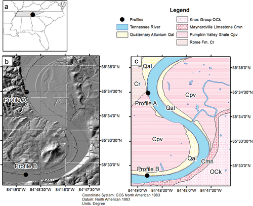
The region that surrounds and drains into the Chickamauga Reservoir is located in the Southern Appalachian Valley and Ridge physiographic area, where the Tennessee River flows southward. The topography of the area consists of northeast-southwest trending ridges and parallel lowland valleys, with elevations ranging from 210 to 305 m a.s.l. The bedrock forming the ridges and valleys are sedimentary rocks of Cambrian- to Ordovician-age and include limestone, dolostone, shale, siltstone, and sandstone of the Rome Formation, Pumpkin Valley Shale, Maynardville Limestone, Knox Group, and Chickamauga Group (Figure 1C) (Hardeman et al., 1966). Stream terraces and floodplains of the Tennessee River unconformably overlie the bedrock and are mapped as Quaternary Alluvium. The two sediment profiles overlie the Pumpkin Valley Shale Formation (Figure 1C). The alluvial material of higher stream terraces was likely deposited during the Pleistocene, whereas the alluvium composing the floodplains of the Tennessee River was likely deposited in the Holocene (Hardeman et al., 1966).

Although impounded by dams in the research area, the Tennessee River is free-flowing (i.e. it is not a static reservoir with no flow annually), carrying silicate-rich sediments eroded from the Valley and Ridge and Blue Ridge Provinces, with provenance from sedimentary, igneous, and metamorphic rocks (USGS, 2001). The upper Tennessee River also drains deeply weathered parts of the Blue Ridge Mountains, eroding micaceous saprolite material that becomes part of the sediment load of the river (Leigh, 2017). Previous characterization of sediment in the Tennessee River and its tributaries showed that suspended sediment in the river is mostly silt and clay-size material, with suspended sediment collected at several stations rarely exceeding 25% sand (Trimble & Carey, 1984).

Materials and methods

Location and sampling of profiles

Field description and initial sampling were conducted in the summer of 2018 at two sites (a cut-bank and a point-bar) identified as outcrops where fluvial sedimentary sequences of paleosols and overbank sediments were well exposed. At each site, the exposures were scraped clean, photographed, and described using standard USDA-NCRS soil terminology (Schoeneberger et al., 2012). Description in the field included characteristics such as consistency, grain-size, soil color, structure, and contacts between layers. Bulk samples of each layer were collected with a trowel and stored in plastic bags in a cold room (~5°C) for charcoal sampling.

Sedimentological analyses

Sedimentological characterization of the soil profiles was done with particle-size analysis (PSA). PSA was performed at the University of Tennessee Archeological Research Laboratory (UT ARL) for 38 samples (profile A n = 18, profile B n = 20), with at least one sample per layer for all the horizons in both profiles. Each sample was intended to be a representative specimen of the bulk sample collected. The samples were analyzed for particle-size distribution using laser diffraction with a Malvern® Mastersizer 3000 particle-size analyzer in wet dispersion mode. Subsamples of about 0.3 g weight were obtained from each bulk sample using a sediment splitter and placed in 50 mL centrifuge tubes that were filled with 25 mL of commercial bleach, vortexed, and placed on a water bath at 80° Celsius overnight to remove organic matter. About 20 mL of the commercial bleach was removed with a syringe from each tube, without disturbing the sediments. To rinse the sediments, sodium hexametaphosphate [40 g/L] was added to fill the tubes to about 25 mL. The samples were vortexed, centrifuged, and again drained with the syringe. The rinsing procedure was repeated three times on each sample. Before analysis, samples were kept in sodium hexametaphosphate to avoid aggregation of clay particles.

Microscopic analysis of oriented thin sections

Samples for oriented soil thin sections were collected using polyvinyl chloride (PVC) squared hollow boxes of 5 cm by 7 cm dimensions for profile A (n = 7) and profile B (n = 6). Boxes were hand-driven into the exposures using a rubber mallet, and then excavated with trowels for removal. Thin sections were prepared commercially and vacuum-impregnated with epoxy. The oriented thin sections were analyzed, and photomicrographs were obtained with an Olympus B×51 Microscope equipped with a Leica 7.6 MPx digital camera at Baylor University, using plane-polarized (PPL) and cross-polarized light (XPL), and UV fluorescence (UVf). The samples were collected in between horizons and in clear contacts between horizons to observe micromorphological differences between the different layers. Entire 5 cm by 7 cm thin sections were photographed with an iPhone 12 Max Pro 12 MPx camera and analyzed with digital imaging software (ImageJ and Photoshop).

Charcoal sampling for radiocarbon dating

Charcoal fragments were hand-picked from sieved sediments and collected in scintillation vials for oven drying at 40° Celsius. In some cases, one single piece of charcoal was enough to make up the minimum amount required for the analysis (2–5 mg). In other cases, several small pieces were hand-picked to make up the mass required. Thirteen AMS radiocarbon determinations were made at the University of Georgia Center for Applied Isotope Studies (UGAMS) (n = 7) and the University of California Irvine – Keck-Carbon Cycle AMS facility (UCIAMS) (n = 6). Radiocarbon dates were calibrated using Calib 8.2 Software (Stuiver, Reimer, and Reimer, 2020) and the Intcal20 dataset of (Reimer, 2020). The 2σ probability ranges are reported in calibrated years before present (cal. yrs. B.P.) and median ages of the 2σ probabilities are reported in 1000s of calibrated years before present (cal. ka B.P.).

Single grain OSL

Single-grain quartz OSL analysis was performed on 16 samples collected from sediments with little evidence of pedogenesis. Four predominantly sandy horizons were targeted and sampled in each of the two profiles. One replicate sample from each of the targeted horizons was taken to analyze effects of partial bleaching and bioturbation in the samples, and to assess the results of OSL dating in the paleosols. OSL samples were collected in October of 2019 following procedures from Nelson et al. (2015) using 5 by 15 cm aluminum liners to avoid sunlight contamination. The samples were processed and analyzed at the Utah State University Luminescence Lab. All samples were opened and processed under dim amber safelight conditions. The samples were wet-sieved to grain-size fractions of 75–150 µm or 150–250 µm, and chemically treated to isolate the quartz fraction. Samples were treated with 10% HCl to remove carbonates and H₂O₂ to remove organic matter. Heavy mineral separation was used to separate the quartz grains from other minerals using a 2.72 g/cm³ solution of sodium polytungstate. A solution of 48% HF was used to remove feldspar and etch the outer layers of the quartz grains affected by alpha radiation. Quartz purity was checked by stimulating aliquots of the samples with infra-red (IR) light to detect the presence of feldspar, HF treatment was repeated until no response to IR-stimulation. Grains with signal-depletion following IR stimulation (Duller, 2003) were not used in analysis.

OSL measurements were performed using an automated Risø TL/OSL luminescence reader (DA-20) following the single-aliquot regenerative-dose protocol (SAR) (Wintle & Murray, 2000). The quartz grains were stimulated using a green laser (532 nm, at 135 mW/cm²) and luminescence was detected through 7.5 mm ultra-violet (UV) filters (U-340). Luminescence signals were measured over 1 s and the signal was calculated for the first 0.05 s subtracting the average of the last two 0.2 s of the luminescence decay. Preheat temperatures following administer and natural doses were 220°C for 10 s and cutheat temperatures following test doses (5–10 Gy) were 160°C for 10 s.

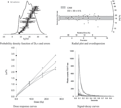
OSL ages for most samples were calculated using a central age model (CAM) (Galbraith & Roberts, 2012). Samples with significant positive skew in D_E value distributions, suggesting partial bleaching, were calculated with the minimum age model (MAM) (Galbraith & Roberts, 2012) (n = 1, profile A, sample 3BC replicate (USU-3373)). Samples with D_E values near zero were calculated using the unlogged CAM following Galbraith and Roberts (2012) (n = 2, profile B, samples Bw (USU-3375) and Bw replicate (USU-3379)). OSL ages are reported at 2σ standard error.

Sediments were collected in proximity to each sample and analyzed for radioisotope concentrations of U, Th, K, and Rb using ICP-MS techniques. These concentration values were converted to dose-rate using conversion factors of Guérin et al. (2011) and beta attenuation values of Brennan (2003). Sample depth, latitude and longitude, and elevation were considered to calculate the contribution of cosmic radiation (Prescott & Hutton, 1994). Dose rates were calculated based on water content, sediment chemistry, and cosmic contribution following Aitken (1998).

Results

Soil profiles and PSA

The Web Soil Survey (USDA, 2001) maps the surface of the two soil profiles as soils from the Staser soil series. The Staser soils mainly occur along the Tennessee River, typically as deep, well-drained, friable and fine sandy loams, with slopes ranging from 0 to 3%, they are dark colored, and have high water capacity and permeability (Warren, 1974). The Staser series soils are taxonomically classified as fine-loamy, mixed, active, thermic Cumulic Hapludolls. The soils in the studied soil profiles fit in part the description of the Staser series because they are well-drained, friable, fine sandy to sandy loams, with slopes ranging from 0 to 3%, with high permeability. However, taxonomically the soils in the profiles have the characteristics of Inceptisols as thermic Psammentic Humudepts because sandy particle-size classes occur in all subhorizons. The two soil profiles were described, sampled, photographed, and dated using radiocarbon and OSL (Appendix 1, Figure 2).

Figure 2. Stratigraphic columns and field photographs with ages obtained from AMS radiocarbon (black font) and OSL (blue font). A) profile a (cut-bank) with zoomed-in photograph of horizons 3Ab/Bt, 3BCb, and 4Ab/Bt. B) profile B (point-bar).

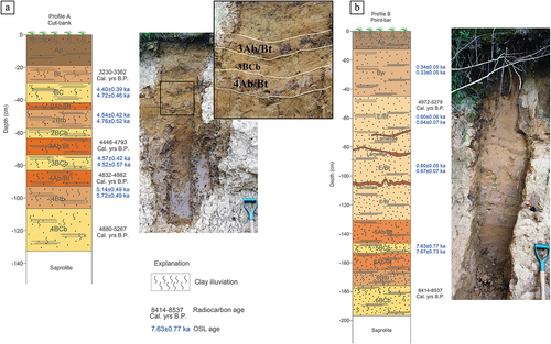
Cut-bank profile

Profile A consists of a vertical sequence of three stacked buried soils that underlie the topsoil column (Appendix 1, Figure 2A). The surface soil (Ap) presents characteristics of a Psammentic Humudept with an ochric epipedon. Below the Ap horizon, an argillic subsoil horizon (Bt) is present followed by an argillic horizon that preserves features of the parent material (BC) and has a lower degree of development than the overlying Bt horizon. The underlying soil columns follow a similar structure as they consist of buried A horizons (Ab/Btb) followed by a buried argillic (Btb) horizon, and/or a buried argillic horizon that preserves features of the parent material (BCb). Buried A horizons for this profile consist mostly of dark brown to light dark brown, fine sandy to sandy loams with angular to subangular blocky ped structure that shifts towards the bottom to angular and strong angular blocky ped structure. There is evidence of clay illuviation and clay coatings in the buried A horizons, which is noted in the nomenclature (Btb). Clay content in the buried A horizons ranges from 4.8 wt. % to 5.7 wt. % and sand content (combination of very fine-, fine-, medium-, coarse-, and very coarse-sand) ranges from 59.1 wt. % to 65.5 wt. % (Appendix 2). Underlying the buried A horizons are lighter colored sandy loams with weak subangular to granular structure and firm to friable consistency. Clay translocation occurs in these horizons, which allows us to identify them as argillic horizons (Btb) (USDA, 2014). Clay content in Btb horizons varies between 5.0 wt. % to 11.3 wt. % and sand content ranges from 35.4 wt. % to 63.6 wt. % (Appendix 2). Btb horizons present illuvial clay accumulation and some iron oxide staining in the sediments. Differences between the Ab and underlying Btb horizons are a darker color present in the Ab horizons compared to the Btb horizons and hardened consistency in the Ab horizons compared to the Btb horizons. The structure in the Ab horizons has greater blocky and angular peds when compared to the firm to friable consistency in the Btb horizons (Figure 2A, zoomed-in photograph). Argillic horizons with characteristics of the parent material (BCb) occur underlying the Btb horizons and in 3BCb directly underlying an Ab horizon. BCb horizons are light yellow, sandy loams with weak subangular to granular structure and friable consistency. Clay content in BCb horizons varies between 3.7 wt. % and 6.0 wt. % and sand content ranges from 59.6 wt. % to 73.3 wt. %.

No carbonate was observed in the sediments based on lack of effervescence with dilute HCl. Fine and medium roots traverse the units, with more and thicker roots in the upper units; however, roots are present in the entire thickness of the profile. Biological activity from insects and worms was observed in the sediments in the form of fecal pellets and burrows. Total thickness of the profile is 150 cm.

Point bar profile

Profile B consists of a vertical sequence of two stacked buried soils that underlie the topsoil column (Appendix 1, Figure 2B). The surface soil (Ap) also presents characteristics of a Psammentic Humudept with an ochric epipedon. Below the Ap horizon, a cambic subsoil horizon (Bw) occurs with some changes in color and structure. The Bw horizon is a brown to orange sandy loam, with weak subangular blocky ped structure, and friable consistency. Following the Bw horizon, a thick E/Bt horizon with clay lamellae occurs. The E/Bt horizon is of light brown color, with weak subangular to granular ped structure, and friable consistency. The clay lamellae occur as thin, undulating horizontal features towards the middle and bottom of the horizon, with three distinct lamellae layers visible with the naked eye. Clay content in the interlamellar layers of the E/Bt horizon range from 3.8 wt. % to 6.7 wt. % and sand content vary between 50.8 wt. % and 70.5 wt. % (Appendix 2). The lamellar layers are dark brown in color with clay content ranging from 4.3 wt. % to 5.9 wt. % and sand content varies between 56.7 wt.% and 66.1 wt. %. Two buried A horizons with evidence of clay illuviation (Ab/Btb) are present towards the bottom of the profile and consist mostly of light dark brown loams. Structure for the Ab horizons varies from strong angular blocky to angular blocky, and consistency is firm. Clay content in the Ab horizons ranges from 3.8 wt. % to 7.1 wt. % and sand content varies between 56.0 wt. % and 65.0 wt. % (Appendix 2). Underlying the two Ab horizons are argillic horizons (Btb) and/or argillic horizons that preserve the characteristics of the parent material (BCb) and have lower degrees of soil development than the overlying Ab or Btb horizons. BCb horizons occur as orange to brown sandy loams with illuvial clay accumulation and subangular to angular blocky ped structure and friable consistency. Clay content in the BCb horizons ranges from 3.0 wt. % to 4.4 wt. % and sand content ranges from 66.6 wt. % to 72.2 wt. % (Appendix 2). No carbonate was observed in the sediments based on lack of effervescence with dilute HCl. Total thickness of the profile is 230 cm. Fine, medium, and thick roots traverse the units, with more and thicker roots in the upper units but roots are present throughout the profile. Biological activity from insects and worms was observed in the sediments as fecal pellets and burrows.

Soil micromorphology

Profile A (cut-bank)

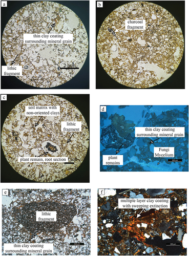
Micromorphological features related to argillic (Bt) or argillic with preserved characteristics of the parent material (BC) horizon development are common in profile A. Illuviated clay is commonly found coating root and animal biopore walls, and surrounding mineral grains and sedimentary rock fragments, forming clay coatings (Figures 3A, 3B, 3C, and 3F). The presence of pedogenic clays was observed in the units from profile A below the topsoil Ap horizon including buried A horizons as accumulations of clays, silt-size quartz grains, and iron oxides. The clay coatings appear dark orange with black and transparent inclusions in PPL (Figures 3A, 3C) and dark orange, gray, and brown birefringent colors with sweeping extinction in XPL (Figures 3B, 3F). The clay coatings do not exhibit UVf (Figure 3D). The paleosols consist of a very fine-grained soil matrix dominated by clay and quartz silt, and Fe oxides. Sand-size sedimentary rock fragments in profile A are scarce but include black to dark brown shale and greenish to white-colored siltstone (Figures 3A, 3B, 3C, 3F). The BC horizons are more porous and contain less soil matrix. However, clay coatings are present in the BC horizons in the same way as they appear in the paleosols. Other components observed in the oriented thin sections are charcoal fragments of sand-size dimensions (Figure 3E), plant remains such as root sections (Figures 3C, 3D), and animal fecal pellets (Figures 4A, 4C).

Figure 3. Photomicrographs of oriented soil thin sections. A) Profile A, contact between Ap and Bt, PPL. Crescent and layered clay coatings composed of clay particles and iron oxides. B) Profile A, contact between Ap and Bt, XPL. C) Profile A, contact between Ap and Bt, PPL. Crescent and layered clay coatings composed of clay particles and iron oxides. Bottom right clay coating shows direction of soil water flow downward. D) Profile A, contact between Ap and Bt, NU. Root section fluorescent under UV. E) Profile A, 4BCb, PPL. Charcoal fragment and loose sand grains. F) Profile A, 3Ab/Bt, XPL. Several crescent clay coatings fill pore walls and coating grains. Well-developed coatings can be observed as the extinction of the clay coatings is the same in several layers of clay.

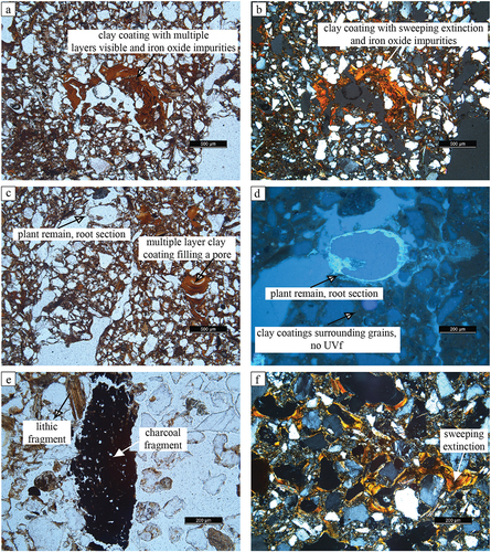
Figure 4. Photographs of whole thin sections for Profile A. Dark red to brownish red features are clay coatings. Spheroidal elements with distinct circular shapes are fecal pellets. Discolorations within the same thin section correspond to evidence of bioturbation as animal burrows. Root casts and walls can be observed as elongated and irregular pore spaces. Black features correspond to fragments of charcoal. A) Contact between Ap and Bt. B) BC. C) 3Ab. D) Contact between 3BCb and 4Ab/Bt. E) Contact between 4Ab and 4Btb. F) 4BCb.

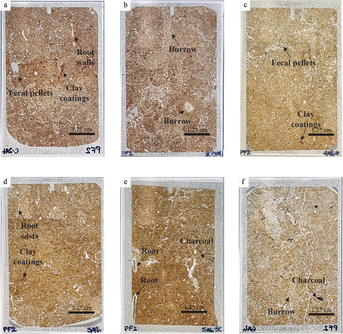
Analysis of 5 cm by 7 cm photographed thin sections (Figure 4) show clear evidence of animal bioturbation as burrows and fecal pellets (Figures 4A, 4B, 4C, 4F). Root walls and casts created by roots can be observed in the thin sections as well (Figures 4A, 4D, 4E). The oriented thin section between the contact of 4Ab/Btb with 4Btb (Figure 4E) contains two fragments of a root alive at the time of sampling. Bioturbation from insects, worms, and plants occurs in all the oriented thin sections, evidenced by reworking of grains, differences in color, and reorganization of grains (Figure 4B, top of the thin section). Thick clay coatings can be observed in the thin sections as reddish to dark brown features that fill pores or accumulate in root walls (Figures 4A, 4C, 4D).

Profile B (point-bar)

Micromorphological features related to changes in structure and color in a weakly developed soil are common in profile B, from the topsoil horizon to the bottom of the E/Bt horizon. Micromorphological features related to argillic horizon (Bt) and argillic horizon with preserved characteristics of the parent material (BC) occur from 5Ab/Btb to the bottom of profile as clay coatings (Figure 5F). The upper units (Bw to E/Bt) show weak soil development accompanied by changes in structure and soil color. The soil matrix is composed of clays, silt-sized quartz grains, and some iron oxides (Figures 5A, 5B, 5C). Clay illuviation has occurred in Bw and clays are present as described in section 5.1.2, but the particles are not organized as clay coatings as they exist mainly surrounding grains and in the soil matrix. Some spaces have thin clay coatings (Figure 5A, upper right space). In the E/Bt horizon, there is clear evidence of clay translocation present as clay lamellae. The clay occurs as particles surrounding grains and in the soil matrix in the interlamellar horizons and more concentrated in the lamellae but are not organized or oriented parallel to the surfaces they adhere to. The clay coatings are not developed in the Bw and E/Bt horizons. The soil matrix is greenish yellow in PPL and reveals dark brown birefringent colors in XPL. Neither the soil matrix nor the thin, weakly developed clay coatings present are fluorescent under Uvf (Figure 5D). The Bw and BCb horizons are more porous and contain less soil matrix. Other components observed in Ab, Bt, and BC horizons are plant remains such as root sections (Figure 5C), charcoal fragments of sand-size dimensions (Figures 5D, 5E, 5F), fungal development as fungal mycelia (Figure 5D), and coarse lithic fragments (Figure 5E). Lower stratigraphic units from 5Ab/Bt to the bottom of the profile (older units) exhibit crescentic, layered clay coatings that are thick and well-developed with a sweeping extinction in XPL. Clay coatings present in these lower units are infilling pore and root walls and surrounding mineral grains (Figure 4F).

Figure 5. Photomicrographs of paleosols and alluvium horizons. A) Profile B, Bw, PPL. Very few crescent and layered clay coatings. Soil matrix surrounding mineral grains of quartz, feldspar, plagioclase, amphibole, and micas. B) Profile B, Bw, PPL. Soil matrix surrounding grains. High clay content. Charcoal fragments of sand grain size. C) Profile B, contact between Bw and E/Bt, PPL. Soil matrix surrounding mineral grains. Root section. D) Profile B, contact between Bw and E/Bt, NU. Charred root section nonfluorescent under UV. Weakly developed thin clay coatings surrounding mineral grains. Fungi Mycelium in bottom of photomicrograph, fluorescent under UV NU light. E) Profile B, E/Bt, PPL. Lithic fragment. F) Profile B, contact between 6Btb and 6BCb, XPL. Several crescent clay coatings fill pore walls and coating grains. Well-developed coatings can be observed as the extinction of the clay coatings is the same in several layers of clay.

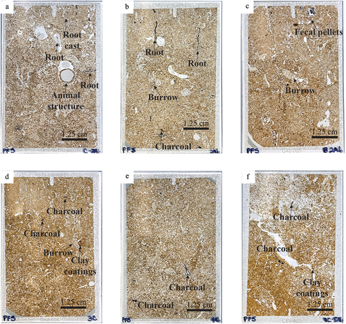
Analysis of the 5 cm by 7 cm photographed thin sections (Figure 6) shows clear evidence of animal bioturbation as burrows, fecal pellets, and animal-created structures (Figures 6A, 6B, 6C, 6D). Root walls and casts created by roots can be observed in the whole thin sections as well. Roots, some of them alive at the time of sampling, are more common in profile B (Figures 6A, 6B). Bioturbation from insects, worms, and plants can be seen in all the oriented thin sections and is evidenced by reworking of grains, differences in color, and reorganization of grains (Figure 6C, middle of the thin section). Thick clay coatings can be observed in the thin sections as reddish to dark brown features that fill pores or accumulate in root walls (Figures 5D, 5F). Large pores are evident in all the thin sections and seem to connect all units throughout the profile.

Figure 6. Photographs of whole thin sections for Profile B. Dark red to brownish red features are clay coatings. Spheroidal elements with distinct circular shapes are fecal pellets. Discolorations within the same thin section correspond to evidence of bioturbation as animal burrows. Root casts and walls can be observed as elongated and irregular pore spaces. Black features correspond to fragments of charcoal. A) Upper Bw. B) Lower Bw. C) Contact between Bw and E/Bt. D) Upper E/Bt. E) Middle E/Bt. F) Contact between 6Btb and 6BCb.

Radiocarbon ages

Radiocarbon analyses on charcoal (Table 1) estimate the ages of the paleosols in profile A (7 dates) as the upper part of the middle Holocene to Late Holocene. The youngest age in the profile corresponds to horizon Bt (21–26 cm) ranging from 3362 to 3230 calibrated (cal.) years before present (B.P.). The oldest age in the profile corresponds to horizon 4BCb (120–127 cm), ranging from 5267 to 4880 calibrated (cal.) years before present (B.P.). The ages at 28–33 cm, 55–60 cm, and 61–69 cm seem to indicate that translocated older charcoal was sampled and analyzed, as the ages are older than expected based on the radiocarbon dating results of the whole profile (Table 1, gray highlighted rows). Based on the results of AMS radiocarbon dating, the sediments in profile A were deposited in a span of about 1700 years.

Table 1. Radiocarbon dates on charcoal in the profiles. Note: Shaded ages shown here are interpreted as ages that are overestimated due to erosion and transport of older charcoal.

Lab	Radiocarbon lab code	Profile	Depth (cm)	Horizon	Stratigraphic context	Conventional radiocarbon age ^a Yrs B.P.	Calibrated median age ^b (ka)^c B.P.	2σ probability ranges Cal yrs B.P. (probability)	Age range with Inbuilt-age ^d Cal Yrs B.P.	Age range for comparison with OSL ^e (Yrs.)
UGAMS	37418	A	21–26	Bt	Argillic horizon	3080±20	3292 (3.3)	3230–3362 (1.000)	3130–3362	3200–3432
UGAMS	37419	A	28–33	BC	Argillic horizon with remanent features of parent material	4470±20	5093 (5.1)	4979–5008 (0.068) 5034–5092 (0.172) 5095–5140 (0.165) 5162–5283 (0.595)	4879–5283	4949–5353
UGAMS	37420	A	55–60	2Btb-2BCb	Contact between argillic horizon and argillic horizon with remanent features of parent material	6690±20	7538 (7.5)	7510–7542 (0.535) 7560–7606 (0.465)	7410–7606	7480–7676
UGAMS	37421	A	61–69	2BCb-3Ab	Contact between argillic horizon with remanent features of parent material and buried A horizon	6300±20	7208 (7.2)	7165–7229 (0.684) 7231–7264 (0.316)	7065–7264	7135–7364
UGAMS	37422	A	70–74	3BCb	Buried A horizon	4080±20	4563 (4.6)	4446–4472 (0.076) 4518–4624 (0.792) 4639–4641 (0.001) 4642–4643 (0.001) 4681–4691 (0.014) 4761–4793 (0.115)	4346–4793	4416–4863
UGAMS	37423	A	90–97	4Ab-4Btb	Contact between A horizon and argillic horizon with remanent features of parent material	4280±20	4848 (4.8)	4832–4862 (1.000)	4732–4862	4802–4932
UGAMS	37424	A	120–127	Middle 4BCb	Argillic horizon with remanent features of parent material	4430±20	5013 (5.0)	4880–4936 (0.092) 4957–5054 (0.729) 5111–5122 (0.012) 5187–5239 (0.128) 5241–5267 (0.039)	4780–5267	4850–5337
UCIAMS	222302	B	50–58	E/Bt	Horizon with lamellae	4455±20	5136 (5.1)	4972–5075 (0.390) 5101–5136 (0.102) 5166–5279 (0.508)	4872–5279	4902–5349
UCIAMS	222303	B	77–83	E/Bt	Horizon with lamellae	7870±20	8636 (8.6)	8592–8724 (0.971) 8739–8754 (0.020) 8757–8764 (0.009)	8492–8764	8462–8834
UCIAMS	222304	B	110–112	E/Bt	Horizon with lamellae	14245±20	17326 (17.2)	17126–17250 (0.241) 17252–17419 (0.759)	17026–17419	17096–17489
UCIAMS	222305	B	118–121	E/Bt	Horizon with lamellae	24420±20	28694 (28.7)	28586–28791 (1.000)	28486–28791	28556–28861
UCIAMS	222306	B	170–180	6Ab/Bt	Buried A horizon	9490±20	10736 (10.7)	10602–10615 (0.016) 10657–10785 (0.806) 10969–11001 (0.122) 11036–11062 (0.056)	10502–11062	10572–11132
UCIAMS	222307	B	190–197	6BCb	Argillic horizon with remanent features of parent material	7685±20	8459 (8.5)	8414–8524 (0.956) 8527–8537 (0.044)	8314–8537	8384–8677

^aConventional radiocarbon age is expressed with standard error in years before present (Yrs B.P.).

^bMedian probability age calculated in Calib 8.2 Software (Stuiver et al., 2020), using the IntCal20 dataset of Reimer (2020).

^cAges in parentheses are rounded to nearest century and expressed as kiloannums (ka) B.P.

^dInbuilt-age error has been added to the calibrated 2σ age range to account for the time gap between carbon fixation and the occurrence of a fire. 100 years have been added to the youngest end of the calibrated age range following Horn and Underwood (2014) and their findings for the Appalachian region.

^eDatum for all ages in the last column is 2020 CE (+70 yr added to all of the BP-1950 calibrated ages after adjusting for inbuilt age).

Results of radiocarbon dating of charcoal in profile B (5 dates) show ages covering the late Pleistocene to the late middle Holocene. The youngest age in the upper part of horizon E/Bt is between 5279 and 4972 cal. years B.P. at 50–58 cm depth. The oldest age in the profile corresponds to the lower part of horizon E/Bt and ranges from 28,791 to 28,586 cal. years B.P. at 118–121 cm depth. Three ages from horizon E/Bt (77–83 cm, 110–112 cm, and 118–121 cm) and one from horizon 6Ab/Btb (170–180 cm) seem to have been obtained from older charcoal eroded from an upstream site, transported, and deposited in the floodplain (Table 1, gray highlighted rows). If the ages considered to be the result of older charcoal redeposited with the flood are omitted from the analysis, profile B would be early to middle Holocene in age. If all the ages are considered, the sediments would be from late Pleistocene to middle Holocene in age.

OSL ages

Results from single-grain OSL in quartz mineral grains of the soil profiles indicate that profile A is significantly older than profile B (Table 2). Ages estimated for profile A range from 5140 ± 490 years to 4400 ± 390 years, indicating the sediments in profile A are upper middle Holocene and were deposited in a span of about 700 years. The ages estimated from the replicates taken in each horizon are also of upper middle Holocene age, ranging from 5720 ± 570 years to 4720 ± 460 years. Compared to the initial samples, the replicates in profile A indicate older ages for the deposits. Age estimates from profile B show the deposits from horizon Bw to E/Bt are all upper late Holocene ranging from 600 ± 50 years to 340 ± 50 years. The OSL age estimated for unit 6BCb is considerably older, 7630 ± 770 years. Results from the replicates in profile B are similar to the ages obtained in the initial samples (Table 2). Over-dispersion in the samples ranges from 7 ± 5% to 57 ± 12% (Table 2).

Table 2. Single-grain OSL ages calculated in quartz grains for the soil profiles.

Profile	Sample Horizon	Lab Code	Depth (m)	Grain-size fraction (µm)	Number of grains^1	Dose rate (Gy/kyr)	Equivalent Dose^2 ± 2σ (Gy)	Over-dispersion (%)	Single-grain OSL age ± 2σ (ka)
A	BC	USU-3028	0.30	75–150	58 (900)	2.83 ± 0.11	12.48 ± 0.86	23 ± 3	4.40 ± 0.39
A	BC replicate	USU-3371	0.30	150–250	37 (1400)	2.86 ± 0.11	13.51 ± 1.48	23 ± 4	4.72 ± 0.46
A	2Btb	USU-3029	0.55	75–150	40 (1400)	2.79 ± 0.11	12.66 ± 1.10	25 ± 4	4.54 ± 0.42
A	2Btb replicate	USU-3372	0.55	150–250	26 (1500)	2.76 ± 0.11	13.15 ± 1.93	33 ± 4	4.76 ± 0.52
A	3Ab/Bt	USU-3030	0.70	75–150	42 (900)	2.80 ± 0.11	12.78 ± 1.18	26 ± 5	4.57 ± 0.42
A	3Ab/Bt replicate	USU-3373	0.70	150–250	27 (1400)	2.72 ± 0.11	12.30 ± 2.12^3	32 ± 6	4.52 ± 0.57
A	4Btb	USU-3031	0.93	75–150	53 (900)	2.79 ± 0.11	14.33 ± 1.45	29 ± 5	5.14 ± 0.49
A	4Btb replicate	USU-3374	0.93	150–250	36 (1400)	2.72 ± 0.11	15.55 ± 1.65	24 ± 5	5.72 ± 0.55
B	Bw	USU-3375	0.25	150–250	37 (1300)	2.75 ± 0.11	0.94 ± 0.23^4	31 ± 9	0.34 ± 0.05
B	Bw replicate	USU-3379	0.25	150–250	41 (1100)	2.75 ± 0.11	0.90 ± 0.25^4	25 ± 6	0.33 ± 0.05
B	Upper E/Bt interlamellae	USU-3376	0.60	150–250	36 (1200)	2.72 ± 0.11	1.64 ± 0.22	7 ± 5	0.60 ± 0.06
B	Upper E/Bt interlamellae replicate	USU-3380	0.60	150–250	24 (1100)	2.72 ± 0.11	1.73 ± 0.28	29 ± 5	0.64 ± 0.07
B	Lower E/Bt interlamellae	USU-3377	0.97	150–250	35 (1200)	3.23 ± 0.13	1.95 ± 0.12^4	57 ± 12	0.60 ± 0.05
B	Lower E/Bt interlamellae replicate	USU-3381	0.97	150–250	34 (1100)	3.23 ± 0.11	2.16 ± 0.25	28 ± 7	0.67 ± 0.07
B	5BCb	USU-3378	1.50	150–250	31 (2000)	2.38 ± 0.11	18.15 ± 2.20	27 ± 5	7.63 ± 0.77
B	5BCb replicate	USU-3382	1.50	150–250	44 (2000)	2.38 ± 0.11	18.26 ± 1.87	30 ± 4	7.67 ± 0.73

^aAge analysis using SAR procedure following Wintle and Murray (2000) on single-grains of quartz sand (G. T. Duller, 2004). Datum for all ages is BP 2020 CE.

^bEquivalent dose (D_E) calculated using the Central Age Model (CAM) following Galbraith and Roberts (2012), unless otherwise noted.

^cEquivalent dose (D_E) calculated using the Minimum Age Model (MAM) following Galbraith and Roberts (2012).

^dEquivalent dose (D_E) calculated using the unlogged CAM following Galbraith and Roberts (2012).

Discussion

Comparison of radiocarbon and OSL ages

Older charcoal fragments can be eroded, transported, and redeposited in fluvial sediments, running the risk of providing older ages than the timing of fluvial deposition (Blong & Gillespie, 1978). The probability of obtaining erroneous ages increases when many small fragments are combined to obtain a single date, as was the case for some of our AMS radiocarbon dates. The combining of multiple fragments for dating and the possibility that some fragments dated were eroded and transported from older deposits likely explain why some radiocarbon ages are much older than OSL ages and are out of order with respect to the stratigraphic position of the units in the soil profiles. Inbuilt-age for charcoal in the southern Appalachians was also considered as a factor that could make AMS radiocarbon ages older than OSL ages. Following Horn and Underwood (2004) we added 100 years to the youngest end of the calibrated age range to account for the time between carbon fixation and the formation of charcoal in a fire, which creates the charcoal fragments that can be transported by streams and incorporated into fluvial deposits (Table 1). The calibrated radiocarbon ages with the inbuilt correction were then converted to have a datum of BP 2020 CE to allow comparison with the OSL ages by adding 70 years to the calibrated age range (difference between BP 1950 and BP 2020 CE). Ages in the discussion are reported as ka (kiloannum).

The age-depth profiles for the radiocarbon and OSL ages at both profiles are presented in Figure 7. In general, there is much greater scatter in the radiocarbon results with depth than seen in the OSL results, which follow an expected increase in age with depth at both profiles. There are several outliers in the radiocarbon ages that are interpreted as being due to transport and deposition of reworked older charcoal (Table 1, gray highlighted rows).

Figure 7. Age-depth diagrams for the two soil profiles based on AMS radiocarbon and OSL ages from Tables 1 and 2. Error bars represent the ± 2σ errors. Black hollow circles correspond to radiocarbon ages, red color stars correspond to OSL ages. A) Profile A. B) Profile B.

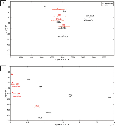
When the radiocarbon older-than-expected outliers are considered, the relationship between OSL and radiocarbon results can be compared. In general, there is good agreement between OSL age and calibrated radiocarbon ages (corrected for inbuilt age and reported as BP 2020 CE) in profile A, although the reported uncertainty on the OSL ages is greater than the calibrated radiocarbon ages (Figure 7A). There is much greater inconstancy between the radiocarbon and OSL results within Profile B (Figure 7B). In the upper part of the profile, the OSL ages are younger than the radiocarbon ages, suggesting that older reworked charcoal was collected from these samples at profile B. The first hypothesis was that ages obtained from AMS radiocarbon dating would yield older ages than OSL because of the time gap between carbon fixation and the time the wood burned, and the possibility of redeposited charcoal, such that OSL would more closely estimate the time of deposition of the flood deposits.

In profile A, ages obtained from OSL are in agreement with the AMS radiocarbon age estimates if the ages that are considered to come for older charcoal transported and redeposited from upstream sites are not taken into consideration. The first hypothesis is supported in profile A as OSL ages seem to more closely reflect the timing of fluvial deposition and it seems that many of the radiocarbon ages are a result of older charcoal transported and redeposited, resulting in ages that are older than the timing of fluvial deposition. Only one sample in profile A (4Ab/Bt-4Btb) seems to be relatively younger than the OSL age (3Btb) but it falls within the 2σ error for the OSL age.

In profile B, the first hypothesis is supported, but with a caveat (Figure 7B). The radiocarbon ages for 25 cm, 60 cm, and 93 cm below surface are significantly older than the OSL ages and the first part of our hypothesis cannot be supported due to the big disparity in the numerical results. It is possible that the radiocarbon ages for 25 cm, 60 cm, and 93 cm in profile B are a result of reworking of older charcoal from other sites and transported and redeposited, and errors due to combining several pieces to make up the minimum weight (5 mg) for processing the samples. The geological studies of the study area indicate that the alluvial materials composing the floodplains of the Tennessee River are likely of Holocene age (Hardeman et al., 1966). Three of the radiocarbon ages in profile B indicate Pleistocene ages that do not agree with the geological studies previously conducted in the study area, and do not agree with the general expectation that the sediments deposited in the point bar profile are younger that the ones deposited in the cut-bank profile. In the lower part of profile B one radiocarbon date in horizon 6Ab/Bt is older than the underlying sample for horizon 6BCb, indicating the possibility of redeposited charcoal in the 6Ab/Bt sample, supporting the first hypothesis.

Single-grain OSL ages from profile A appear to be slightly older than radiocarbon ages from the same section. While this difference is within error of the dating results, it could be that the OSL results were affected by slight partial bleaching (incomplete luminescence resetting), as suggested by our second hypothesis. We observed evidence for positive skew of the equivalent dose (D_E) values, suggesting partial bleaching, in two samples in the profiles. The OSL age 3Ab/Bt replicate from profile A and the lower E/Bt interlamellae sample from profile B show evidence for positive skew of the D_E. The rest of the OSL samples show over-dispersion values that are within typical values for single-grain data (<30%) (Table 2, Appendix 3).

Our samples showed similar values for U, Th, Rb, and K (Appendix 4), indicating high parent material homogeneity, which was also observed in the micromorphological analysis. The parent material homogeneity observed in soil micromorphology and the values for U, Th, Rb, and K indicated that the majority of the quartz grains come from fluvial deposition from the Tennessee River sediment load and not from other sources.

Our second hypothesis was not supported, as only two samples, one in each profile, show positive skew of the D_E and the rest OSL samples show over-dispersion values that are typical for single-grain OSL data.

Soil micromorphology as a tool to evaluate reliability of dating methods

The micromorphological analysis of the oriented soil thin sections showed that a common pedological feature observed in both profiles is argillans or clay coatings. Clay coatings are accumulations of illuviated (translocated) clay particles that were removed from upper horizons and accumulated in pore spaces and surrounding mineral grains. As the clay particles accumulate, they are reorganized and orient parallel to the surface with which they are associated (Stoops & Vepraskas, 2003; Stoops et al., 2010). The presence of illuviated clay in the profiles indicates that the soils are moderately permeable and well drained, as was observed in the field. Another evidence of the soils in the profiles being well drained is the evidence of root pores which can be seen in the photographs of the 5 cm by 7 cm thin sections without magnification (Figures 4 and 6) and in the microscopic analysis (Figures 3 and 5). The evidence of root pores indicates that water was able to infiltrate the soil and transport clay particles downwards in the profile. Clay illuviation is a downward movement that can be as deep as several meters (Buurman et al., 1998), which is visible in the profiles as clay particles seem to be translocating from the upper units to the bottom of the profiles, building up thicker, more developed clay coatings in the older units.

In profile A, clay coatings are abundant, layered, well-developed, and thick (Figures 4A, 4B, 4C, 4F). The well-developed clay coatings in profile A would possibly require thousands of years of pedogenesis to form and enough time for the clay particles to orient. Abundant, thick, and well-developed clay coatings presenting several layers can take thousands of years to form and develop and can provide relative ages for buried soils following Ufnar (2007). The thick, well-developed clay coatings in profile A are supported by the AMS radiocarbon ages (~3.1 ka to~5.2 ka) and the OSL ages (~4.4 ka to~5.72 ka) estimated for the profile.

In contrast, profile B contains some clay coatings that are thin, poorly developed, and scarce in the upper units (Bw and E/Bt) (Figures 5A, 5B, 5C) that shift to thick, abundant, well-developed clay coatings in the lower units (5Ab/Bt to 6BCb) (Figure 5F). The presence of poorly developed thin clay coatings or complete absence of them, and the presence instead of non-oriented clay particles surrounding mineral grains indicates that pedogenesis has not been acting long in the upper units. These observations are consistent with the 0.33–0.67 ka OSL ages from the upper portions of Profile B (Table 1, Figure 7B). Radiocarbon ages from profile B (5–28 ka) are all older than the single-grain OSL ages and suggest they were derived from re-deposited charcoal.

Buried soils in the lower portion of profile B (5Ab/Bt and deeper) have well-developed clay coatings and indicate longer periods of soil formation (Figure 5F). The older ages in the lower units of the profile as reflected in the clay coatings are supported by the AMS radiocarbon ages to (~8.5 ka >5.2 ka) and the OSL ages (~7.63 ka). The difference in OSL ages from the upper to the lower units in profile B indicates that there is a gap (unconformity) in the sedimentary record within the profile, likely from erosion of the alluvial sediment. The wavy or crenulated boundaries between the paleosols, noted in the field description (Appendix 1), provide evidence of erosion (scour) between the deposition of the new units atop the paleosols.

Rates of argillic Bt horizon formation for the southeastern United States vary. In West Virginia, Bt horizons have been recognized in artificial mounds constructed 2.1 ka (Birkeland, 1984). In the Blue Ridge mountains of northern Georgia, a study of a soil chronosequence estimated that it can take about 5000 years for a Bt horizon with well-developed clay coatings to form (Leigh, 1996). Other studies in floodplain soils from the Holocene in Tennessee indicate that well-developed clay coatings require 4000–5000 years to form (Driese et al., 2008). The presence of lamellae in horizon E/Bt in profile B supports some clay illuviation has occurred in <1000 years, but for well-developed clay coatings to form, such as the ones occurring in profile A and in the lower units in profile B, it can take about 4000 years, agreeing with previous studies.

The radiocarbon and OSL ages in between horizons are not more than a thousand years for the radiocarbon ages and some hundreds of years for the OSL ages. For example, AMS radiocarbon ages 3BCb (~4.52–4.86 ka) and 4Ab/Bt-4Btb (~4.90 ka), or OSL ages 2Bt (~4.54 ka) and 3Ab (~4.57 ka) in profile A. Or OSL ages Bw (~0.34 ka) and Upper E/Bt (~0.60 ka) in profile B. It seems that the formation and development of clay coatings does not stop when new units are deposited on top of buried A horizons but continue with time because the paleosols and sediments in the profiles are well drained, permeable, and porous. Other previous works have explained the interactions between sedimentation and pedogenesis and support our model for clay coating formation and development (e.g. Almond & Tonkin, 1999; McDonald & Busacca, 1990). If the formation of clay coatings was interrupted once a new depositional event occurred and buried the previous soil column, formation of Bt horizons would have been limited to a thousand years or less and we would be seeing thick, moderately developed, and abundant clay coatings forming in the E/Bt horizon in profile B. The clay coatings present in Ab, Bt, and BC horizons show that clay translocation seems to be a continuous process and clay particles can move downward not only through Bt and BC horizons but also in Ab horizons. The amount of illuviated clay increases towards the lower units of the profiles where the clay particles continue to move downward and accumulate in biopore walls and surrounding grains (Figure 8). Another evidence of the continuous movement of clay particles through the profile is the clay content in the horizons. If Bt and clay coating development were constrained to when each soil column was exposed, clay contents would be significantly higher in the Bt and BC horizons and depleted in the A horizons. However, clay content in the Ab horizons do not differ drastically from the Bt and BC horizons in either of the soil profiles.

Figure 8. Schematic diagram of clay coating formation in both soil profiles. A) Pedogenesis starts forming soil and soil column develops three horizons, surface soil (Ap), argillic horizon (Bt), and parent material with argillic horizon features (BC). K-feldspar (Kfs), plagioclase (Pl), and muscovite (Ms) start to weather into clay minerals. Clay particles are also available as sediment load from the river. Clay particles travel downward when water infiltrates the soil. During drying periods, clay particles adhere parallel to mineral grain and biopore surfaces, forming clay coatings. B) a depositional event buries the initial soil column, and pedogenesis starts to act in the new fluvial deposits and continues to act in the initial fluvial deposits. Kfs, Pl, and Ms continue to chemically weather into clay minerals, that together with clay carried as suspended sediment from the river continue traveling downwards with water infiltration. New clay coatings form in mineral grain and biopore surfaces in the newer deposits. Older clay coatings receive more clay particles that keep adding and forming thick, and well-developed clay coatings. High permeability, porosity, and well-drained soils allow the newer and the older fluvial deposits to be connected after depositional events.

The micromorphology of the samples supports our third hypothesis that thick, abundant, well-developed clay coatings would support old ages in paleosols, and researchers should pay close attention to amounts and degrees of development of clay coatings when using micromorphology while engaged in floodplain studies. Older paleosols have thick, well-developed clay coatings and plagioclase and feldspar have started to alter to sericite and kaolinite, respectively. In contrast, the paleosols that are recent (0.6 ka to 0.3 ka) have scarce, thin, and poorly developed clay coatings. The OSL and radiocarbon ages in the Bt and BC horizons in our study are consistent with estimates of at least 4000 years for the formation of well-developed, thick, and abundant clay coatings in Bt horizons in the southeastern United States (Driese et al., 2008; Leigh, 1996) in well-drained, permeable, and porous soils where clay translocation continues even when newer units are deposited on top. In the case of profile B, clay lamellae can be a product of depositional processes over pedogenesis. It is possible that the lack of thick, well-developed clay coatings in the thin sections in E/Bt reflect a depositional origin as clays occur as suspended load in the Tennessee River’s sediments and the young age for E/Bt indicates that not enough time has passed for the clays in the lamellae to reorient and reorganize to form thick clay coatings. Thick, well-developed clay coatings are present in the thin sections below horizon 5Ab/Bt where time allowed their formation.

The micromorphological analyses also confirm the rejection of the AMS radiocarbon ages of 17.2 ka and 28.7 ka as inaccurate ages for the fluvial events that resulted from older charcoal being transported and deposited in the flood event. In a temperate humid environment such as the watershed of the Tennessee River, chemical weathering should have degraded plagioclase and feldspar mineral grains into sericite and kaolinite in 17 ka to 20 ka years of pedogenesis. But our analysis of oriented soil thin sections showed mineral grains of feldspar and plagioclase virtually unaltered in profile B, a finding wholly inconsistent with radiocarbon ages from the late Pleistocene.

It is important to note how the degree of development of the soils as observed in the field from structure and consistency, and micromorphology can contribute to the assessment of the reliability of the radiocarbon and OSL ages. In profile A, Bt horizons show development of argillic horizon characteristics, such as changes in structure and color, which not only support older ages for paleosols but also there should have been prolonged periods of exposure to allow the Bt horizons to mature. The clay coatings also need periodic drying for the clay coatings to adhere to the surfaces (Buurman et al., 1998). In between depositional events, long periods of relative stability for soil formation and development and clay coating formation can be inferred. Weakly developed soils in the upper units of profile B support younger ages because there have only been changes in structure and color of the soils. It is possible that for the recent deposits, there has not been a long period of relative stability in between depositional events to allow for the formation of thicker, well-developed clay coatings. In the lower part of profile B, clay coatings are abundant, thick, and well-developed, and the soils are moderately to well developed as evidenced by the changes to angular structure, firm consistency, and argillic horizon development.

Our fourth hypothesis was that bioturbation could have affected both AMS radiocarbon and OSL age estimates. Bioturbation seems to be present in both profiles and has influenced reworking of the grains as observed in the thin sections (Figures 4 and 5). The oriented soil thin sections show that there is abundant heterogeneity in the soils. Features such as burrows (Figures 4B, 4F, 5C, 5D) possibly contain grains that have been moved up and down in the profile. This could be potentially problematic in single grain OSL. Other issues could be vertical movement of particles in the root pores that could affect age estimates for OSL and cause high values of over-dispersion measures. The presence of fecal pellets in the soils (Figures 4A, 4C, 5C) also indicates that invertebrates are present in the soils and bioturbation from invertebrates’ activity should be considered in the analyses of OSL age estimates. The over-dispersion values in the single-grain OSL ages are within what is expected for samples with partial bleaching and the target horizons are thick enough that insect activity is not significant to alter the OSL results. In both profiles, horizons are still distinguishable from one another, with clear boundaries, indicating that bioturbation in between units has not occurred. Bioturbation influence on single-grain OSL ages would be more significant in horizons that are closer to the surface because animal and worm burrows, and insect activity might allow sunlight to reach some of the quartz grains but not in our deposits. The position of the OSL samples well below the surface and the thickness of the target horizons do not support our hypothesis that bioturbation could have altered the estimates for the AMS radiocarbon and OSL ages in both profiles.

Conclusion and recommendations

Comparison of ages obtained from AMS radiocarbon dating of charcoal fragments and OSL dating of quartz grains and examination of soil micromorphology in two sediment profiles in the Upper Tennessee River basin showed that AMS radiocarbon ages are mostly affected by reworking of charcoal from older sites upstream. Single-grain OSL results largely showed consistent ages and the over-dispersion were within typical values for single-grain OSL. Micromorphological analyses provided a basis for assessing the reliability of the ages from both methods. From our findings in this study, and our previous work (Horn & Underwood, 2014) using radiocarbon dating for a variety of organic materials in soils and sediments, we offer the following comments and recommendations for using radiocarbon or OSL in flood deposits and soils.

1. Charcoal can persist in soils or sediments for thousands of years, while non-charred organics are more likely to decompose. If fluvial deposits contain non-charred wood or leaves, we recommend dating this material rather than charcoal. If large pieces of wood are recovered, and it is possible to determine the outer surface of original pieces of woody stems or branches, AMS dates on material near the outer surfaces are better than dates near the center of stem.

2. Charcoal can provide accurate dates on flood events if the charcoal was produced close to the time of the flood and traveled from a burn site to the sampling site without having first been incorporated into upstream slopes or fluvial deposits. Whereas the history of charcoal may be impossible to estimate, dating a number of single fragments of charcoal rather than combining multiple fragments to form a composite sample may be a more reliable method. Dates determined from single fragments of charcoal would provide a distribution of age dates, with the youngest dates expected to be the values that are most reliable. This type of sampling and testing would eliminate the possibility of a few very old fragments skewing the age measured in a composite sample.

3. Partial bleaching is an important factor to consider when OSL dating fluvial deposits. Single-grain OSL dating can help highlight the grain-to-grain scatter due to partial bleaching. Although the OSL ages are within the error of the calibrated radiocarbon ages, there may be some influence of partial bleaching on the OSL results.

4. Bioturbation from plants and animals can affect age estimates in single-grain OSL, if there is evidence of vertical movement of sand-size grains in a profile in horizons that are thin and might be mixed with other age deposits or close to the surface. Whereas it might be difficult to assess the extent to which mineral grains can migrate up or down profile from plant or insect and worm activities, the possibility of mineral grain movement should be considered when there is evidence of bioturbation in soils and alluvium in superficial deposits or deposits of different ages that are a few cm.

5. Pedological features examined microscopically with soil micromorphology can give initial information on depositional settings, history of development of buried soils, and estimated ages for buried soils if the pedological features take thousands of years to form. Although soil micromorphological analysis do not produce numerical ages, they can help establish relative ages and provide a key basis for assessing the reliability of OSL and radiocarbon dates on fluvial deposits.

Disclosure agreement

No potential conflict of interest was reported by the authors.

Acknowledgments

We appreciate the assistance of Howard Cyr with fieldwork. The authors would like to thank the Electric Power Research Institute (grant number 10005236), which provided major funding to the project. We would also like to thank the Tennessee Water Resources Research Institute (2019 USGS 104b Graduate Student Supplemental Research Grant Program), Donald and Florence Jones Professorship Endowment, and the University of Tennessee College of Arts and Sciences for supplemental funding.

Disclosure statement

No potential conflict of interest was reported by the authors.

Data availability statement

The authors confirm that the data supporting the findings of this study are available within the article and its supplementary materials.

Additional information

Funding

The work was supported by the Electric Power Research Institute [10005236]; Tennessee Water Resources Research Center [2019 USGS 104b].

Appendix Appendix 1.

Soil Profile Descriptions

Table

Soil or paleosol	Depth	Description
Profile A (cut-bank)
Ap	0–19 cm	Topsoil. Dark brown (10 YR 3/3) sandy loam; weak subangular blocky ped structure, friable; many fine roots and several wide roots, abundant plant activity; clear and crenulated boundary.
Bt	19–29 cm	Light dark brown (10 YR 4/4) sandy loam; weak subangular blocky structure, friable; some fine roots; abrupt and wavy boundary. Illuviated clay as clay coatings observed in thin section.
BC	29–41.5 cm	Light dark brown (10 YR 3/4) silt loam; weak subangular blocky ped structure; friable; abrupt and crenulated boundary. Illuviated clay as clay coatings observed in thin section.
2Ab/Bt	41.5–46 cm	Buried A horizon. Dark brown (10 YR 3/3) sandy loam; single grain structure; very friable; abrupt and wavy boundary.
2Btb	46–57 cm	Light dark brown (10 YR 4/4) sandy loam; weak subangular blocky ped structure; friable; abrupt and crenulated boundary. Illuviated clay as clay coatings observed in thin section.
2BCb	57–63 cm	Yellowish dark brown (10 YR 4/6) sandy loam; weak subangular blocky structure; friable to very friable; abrupt and wavy boundary. Illuviated clay as clay coatings observed in thin section.
3Ab/Bt	63–74 cm	Buried A horizon. Dark brown (10 YR 3/3) sandy loam; angular blocky ped structure; firm; iron oxide staining; abrupt and crenulated boundary.
3BCb	74–83 cm	Bronze (10 YR 4/6) sandy loam; granular structure; very friable consistence; iron oxide staining; abrupt and wavy boundary. Illuviated clay as clay coatings observed in thin section.
4Ab/Bt	83–93 cm	Buried A horizon. Dark brown (10 YR 3/3) sandy loam; weak angular blocky ped structure; friable; abrupt and crenulated boundary.
4Btb	93–106 cm	Yellowish dark brown (10 YR 4/6) sandy loam; strong angular blocky ped structure; very friable; abrupt and smooth boundary. Illuviated clay as clay coatings observed in thin section.
4BCb	106–132 cm	Light dark brown (10 YR 3/4) sandy loam; granular structure; firm; abrupt boundary. Illuviated clay as clay coatings observed in thin section.
Profile B (Point-bar)
Ap	0–12.5 cm	Topsoil. Very dark brown (10 YR 3/2) fine sandy loam; granular to weak subangular blocky ped structure; very friable; many thin and wide roots, abundant plant activity; clear and smooth boundary.
Bw	12.5–45 cm	Yellowish dark brown (10 YR 4/6) sandy loam; granular to weak subangular blocky ped structure; very friable; several thin roots; clear and smooth boundary.
E/Bt	45–130.5 cm	Light dark brown (10 YR 3/4) fine sandy loam; angular blocky ped structure; firm; some thin roots; clear and smooth boundary. Presence of dark colored lamellae in this horizon. Translocated clay observed in thin section.
5Ab/Bt	130.5–147 cm	Buried A horizon. Light dark brown (10 YR 4/4) loam; angular blocky ped structure; firm; clear and smooth boundary.
5BCb	147–153.5 cm	Light dark brown (10 YR 4/4) sandy loam; strong angular blocky ped structure; firm; clear and wavy boundary. Illuviated clay as clay coatings observed in thin section.
6Ab/Bt	153.5–165 cm	Buried A horizon. Light dark brown (10 YR 4/4) sandy loam; angular blocky structure; friable; abrupt and wavy boundary. Illuviated clay as clay coatings observed in thin section.
6Btb	165–176 cm	Yellowish dark brown (10 YR 4/6) sandy loam; subangular blocky ped structure; friable consistence; abrupt and wavy boundary. Illuviated clay as clay coatings observed in thin section.
6BCb	176–197 cm	Light dark brown (10 YR 4/4) loam; angular blocky ped structure; friable to slightly firm consistence; roots casts extending downward. Illuviated clay as clay coatings observed in thin section.

Appendix 2.

Results Of PSA

Table

Grain size distribution (wt%)
Soil horizon	Clay	Silt	Very fine sand	Fine sand	Medium sand	Coarse sand	Very coarse sand
Profile A (cut-bank)
Ap	5.7	35.2	25.2	25.2	8.6	0.2	0.00
Bt	5.6	31.9	25.0	27.3	10.1	0.1	0.00
Bt	11.3	53.3	23.4	9.4	1.8	0.8	0.00
BC	5.2	32.1	26.4	27.1	9.1	0.2	0.00
2Ab/Bt	5.1	29.8	26.9	28.0	9.7	0.4	0.00
2Btb	5.0	31.4	26.7	27.6	9.1	0.2	0.00
2BCb	4.4	28.7	27.2	29.5	10.1	0.2	0.00
3Ab/Bt	5.5	30.5	28.0	27.0	8.7	0.3	0.00
3Ab/Bt	5.4	31.3	31.1	25.3	6.7	0.2	0.00
3BCb	3.7	23.1	30.1	33.0	10.0	0.2	0.00
4Ab/Bt	4.8	29.8	28.3	28.0	8.9	0.3	0.00
4Btb	5.4	31.0	28.4	26.9	8.2	0.2	0.00
4Btb	5.5	33.1	28.0	25.6	7.7	0.2	0.00
4Btb	6.2	34.4	27.4	25.6	6.4	0.0	0.00
4BCb	6.0	34.4	28.0	25.2	6.4	0.1	0.00
4BCb	7.1	38.8	27.2	21.2	5.5	0.2	0.00
Profile B (point-bar)
Ap*	-	-	-	-	-	-	-
Bw*	-	-	-	-	-	-	-
E/Bt	6.18	38.01	28.29	22.07	5.16	0.28	0.00
E/Bt	6.72	42.48	28.20	18.75	3.80	0.05	0.00
E/Bt	6.60	41.17	29.04	19.50	3.55	0.14	0.00
E/Bt	6.00	37.43	29.44	22.51	4.49	0.13	0.00
Lamellae	5.77	37.11	28.76	23.07	5.19	0.10	0.00
E/Bt	5.85	37.05	27.96	23.34	5.70	0.09	0.00
Lamellae	5.87	37.46	25.66	23.37	7.45	0.20	0.00
E/Bt	4.83	32.11	24.68	27.70	10.40	0.28	0.00
Lamellae	4.33	29.60	24.20	29.37	11.95	0.55	0.00
E/Bt	3.82	27.23	24.51	31.31	12.67	0.46	0.00
E/Bt	3.79	25.68	25.64	32.36	12.20	0.33	0.00
E/Bt	4.07	27.71	26.62	30.19	10.94	0.47	0.00
5Ab/Bt	4.40	30.63	27.80	27.83	9.14	0.19	0.00
5BCb	4.39	29.04	23.48	28.05	14.15	0.89	0.00
6Ab/Bt	6.09	37.98	21.81	19.92	13.03	1.17	0.00
6Btb	3.05	24.71	16.26	28.82	24.60	2.57	0.00
6BCb	7.07	39.13	21.58	20.36	11.06	0.79	0.00

*Ap and Bw horizons in profile B were significantly mixed by plant roots and the horizons were hanging from the roots. Bulk samples from these two horizons were not taken, but a differentiation between the modern topsoil and the underlying Bw horizon was visible.

Appendix 3.

Equivalent Dose (D_E) Distributions: Probability Density Function, Radial Plot, Overdispersion (OD)

PROFILE A, SAMPLE BC (USU-3028), n = 58 (900).

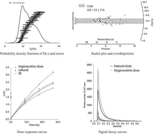
PROFILE A, SAMPLE BC replicate (USU-3371), n = 37 (1400).

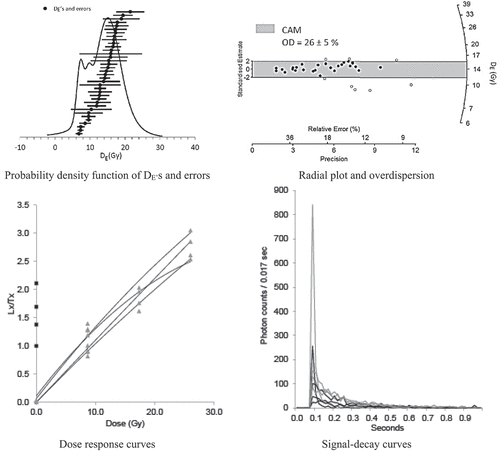
PROFILE A, SAMPLE 2Btb (USU-3029), n = 40 (1400).

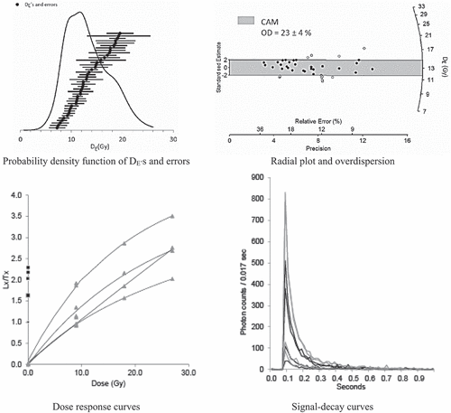
PROFILE A, SAMPLE 2Btb replicate (USU-3372), n = 26 (1500).

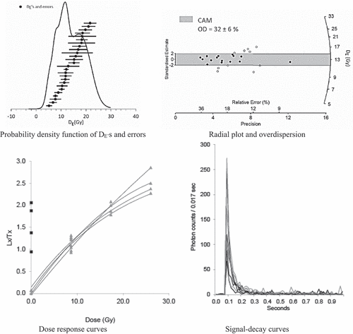
PROFILE A, SAMPLE 3Ab/Bt (USU-3030), n = 42 (900).

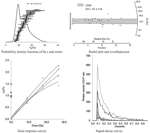
PROFILE A, SAMPLE 3Ab/Bt replicate (USU-3373), n = 27 (1400).

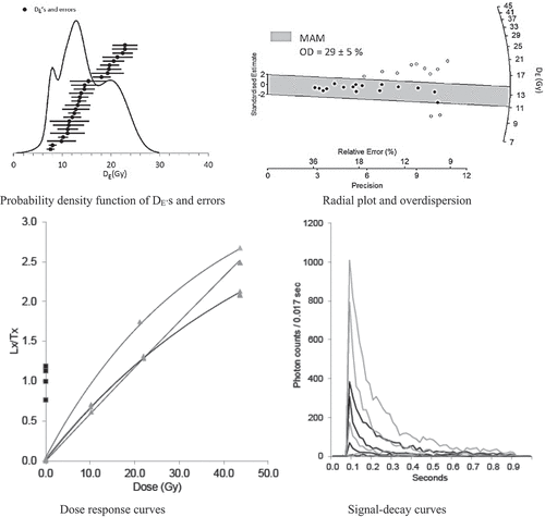
PROFILE A, SAMPLE 4Btb (USU-3031), n = 53 (900).

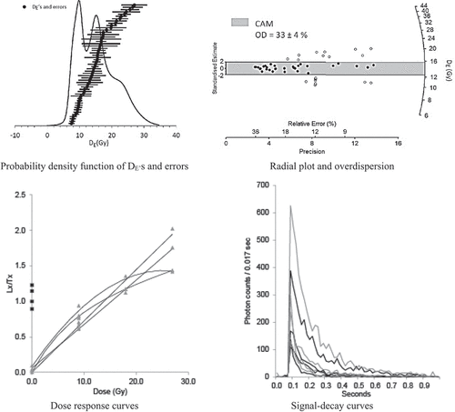
PROFILE A, SAMPLE 4Btb replicate (USU-3374), n = 36 (1400).

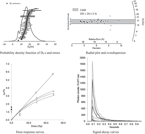
PROFILE B, SAMPLE Bw (USU-3375), n = 37 (1300).

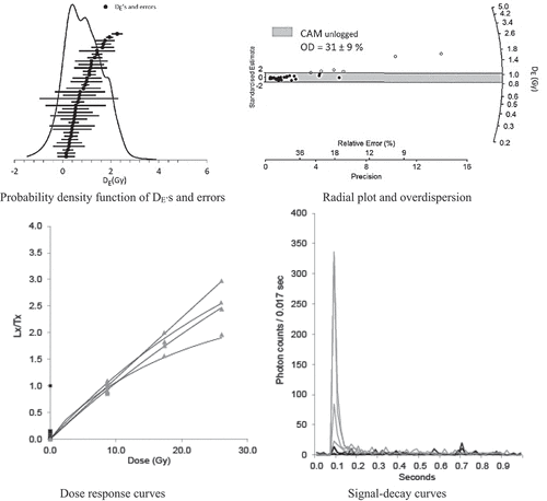
PROFILE B, SAMPLE Bw replicate (USU-3379), n = 41 (1100).

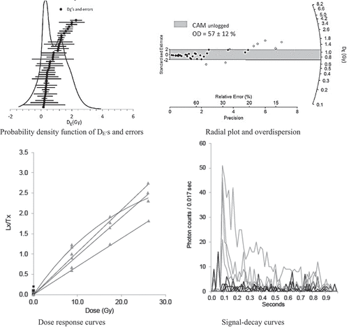
PROFILE B, SAMPLE Upper E/Bt interlamellae (USU-3376), n = 36 (1200).

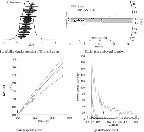
PROFILE B, SAMPLE Upper E/Bt interlamellae replicate (USU-3380), n = 24 (1100).

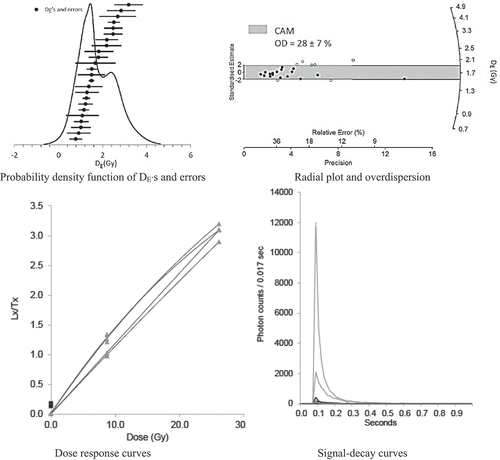
PROFILE B, SAMPLE Lower E/Bt interlamellae (USU-3377), n = 35 (1200).

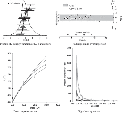
PROFILE B, SAMPLE Lower E/Bt interlamellae replicate (USU-3381), n = 34 (1100).

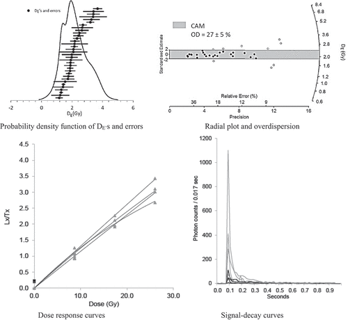
PROFILE B, SAMPLE 5Bcb (USU-3378), n = 31 (2000).

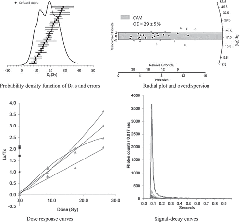
PROFILE B, SAMPLE 5Bcb replicate (USU-3382), n = 44 (2000).

Appendix 4.

Dose Rate (Dr) Information For Single-Grain OSL Samples

Table

Profile	Sample Horizon	Lab Code	In-situ water content^1 (%)	Dose rate horizons	Gamma DR proportion^2	K (%)^3	Rb (ppm) ^3	Th (ppm) ^3	U (ppm) ^3	Cosmic (Gy/kyr)
A	BC	USU-3028	16.8	BC2 C2 BC3	0.25 0.45 0.30	1.74 ± 0.04 1.75 ± 0.04 1.68 ± 0.04	75.9 ± 3.0 81.4 ± 3.3 83.4 ± 3.3	10.1 ± 0.9 10.3 ± 0.9 11.0 ± 1.0	2.3 ± 0.2 2.4 ± 0.2 2.4 ± 0.2	0.21 ± 0.02
A	BC replicate	USU-3371	13.5	C BC2	0.50 0.50	1.84 ± 0.05 1.74 ± 0.04	75.9 ± 3.0 76.9 ± 3.1	10.1 ± 0.9 10.3 ± 0.9	2.3 ± 0.2 2.4 ± 0.2	0.21 ± 0.02
A	2Btb	USU-3029	21.2	BC3 C3 BC4	0.30 0.50 0.20	1.68 ± 0.04 1.75 ± 0.04 1.80 ± 0.04	83.4 ± 3.3 77.1 ± 3.1 84.8 ± 3.4	11.0 ± 1.0 10.0 ± 0.9 10.6 ± 1.0	2.2 ± 0.2 2.4 ± 0.2 2.3 ± 0.2	0.20 ± 0.02
A	2Btb replicate	USU-3372	18.6	BC3 C3 BC4	0.25 0.45 0.30	1.74 ± 0.04 1.75 ± 0.04 1.68 ± 0.04	75.9 ± 3.0 81.4 ± 3.3 83.4 ± 3.3	10.1 ± 0.9 10.3 ± 0.9 11.0 ± 1.0	2.3 ± 0.2 2.4 ± 0.2 2.4 ± 0.2	0.21 ± 0.02
A	3Ab/Bt	USU-3030	23.2	BC4 C4 BC5	0.30 0.30 0.40	1.80 ± 0.05 1.73 ± 0.04 1.80 ± 0.05	84.8 ± 3.4 74.3 ± 3.0 83.5 ± 3.3	10.6 ± 1.0 10.1 ± 0.9 11.1 ± 1.0	2.3 ± 0.2 2.2 ± 0.2 2.5 ± 0.2	0.19 ± 0.02
A	3Ab/Bt replicate	USU-3373	22.9	BC4 C4 BC5	0.30 0.50 0.20	1.68 ± 0.04 1.75 ± 0.04 1.80 ± 0.05	83.4 ± 3.3 77.1 ± 3.1 84.8 ± 3.4	11.0 ± 1.0 10.0 ± 0.9 10.6 ± 1.0	2.4 ± 0.2 2.2 ± 0.2 2.3 ± 0.2	0.20 ± 0.02
A	4Btb	USU-3031	22.6	BC5 C5 BC6	0.35 0.35 0.30	1.68 ± 0.04 1.75 ± 0.04 1.80 ± 0.05	83.4 ± 3.3 77.1 ± 3.1 84.8 ± 3.4	11.0 ± 1.0 10.0 ± 0.9 10.6 ± 1.0	2.4 ± 0.2 2.2 ± 0.2 2.3 ± 0.2	0.20 ± 0.02
A	4Btb replicate	USU-3374	23.2	BC5 C5 BC6	0.35 0.35 0.30	1.80 ± 0.05 1.79 ± 0.04 1.77 ± 0.04	83.5 ± 3.3 73.1 ± 2.9 72.4 ± 2.9	11.1 ± 1.0 9.4 ± 0.8 9.3 ± 0.8	2.5 ± 0.2 2.2 ± 0.2 2.2 ± 0.2	0.19 ± 0.02
B	Bw	USU-3375	10.4	Ap Bw Bw/C2	0.25 0.50 0.25	1.47 ± 0.04 1.64 ± 0.04 1.96 ± 0.04	57.7 ± 2.3 65.4 ± 2.6 81.1 ± 3.3	9.1 ± 0.8 9.9 ± 0.9 9.7 ± 0.9	2.1 ± 0.1 2.3 ± 0.2 2.6 ± 0.2	0.21 ± 0.02
B	Bw replicate	USU-3379	10.1	Ap Bw Bw/C2	0.25 0.50 0.25	1.47 ± 0.04 1.64 ± 0.04 1.96 ± 0.04	57.7 ± 2.3 65.4 ± 2.6 81.1 ± 3.3	9.1 ± 0.8 9.9 ± 0.9 9.7 ± 0.9	2.1 ± 0.1 2.3 ± 0.2 2.6 ± 0.2	0.21 ± 0.02
B	Upper E/Bt Interlamellae	USU-3376	11.8	Bw/C2 C2 Bw/C3 C3	0.25 0.50 0.125 0.125	1.96 ± 0.05 1.74 ± 0.04 1.93 ± 0.05 2.15 ± 0.05	82.1 ± 3.3 70.1 ± 2.8 80.6 ± 3.2 97.5 ± 3.9	9.7 ± 0.9 8.0 ± 0.7 9.9 ± 0.9 12.0 ± 1.1	2.6 ± 0.2 2.0 ± 0.1 2.5 ± 0.2 2.9 ± 0.2	0.21 ± 0.02
B	Upper E/Bt Interlamellae replicate	USU-3380	11.9	Bw/C2 C2 Bw/C3 C3	0.25 0.50 0.125 0.125	1.96 ± 0.05 1.74 ± 0.04 1.93 ± 0.05 2.15 ± 0.05	82.1 ± 3.3 70.1 ± 2.8 80.6 ± 3.2 97.5 ± 3.9	9.7 ± 0.9 8.0 ± 0.7 9.9 ± 0.9 12.0 ± 1.1	2.6 ± 0.2 2.0 ± 0.1 2.5 ± 0.2 2.9 ± 0.2	0.21 ± 0.02
B	Lower E/Bt Interlamellae	USU-3377	14.2	C2 Bw/C3 C3 Bw/C4	0.25 0.50 0.125 0.125	1.93 ± 0.05 2.15 ± 0.05 2.07 ± 0.05 1.74 ± 0.04	80.6 ± 3.2 97.5 ± 3.9 96.4 ± 3.9 70.1 ± 2.8	9.9 ± 0.9 12.0 ± 1.1 12.9 ± 1.2 8.0 ± 0.7	2.5 ± 0.2 2.9 ± 0.2 2.9 ± 0.2 2.0 ± 0.1	0.20 ± 0.02
B	Lower E/Bt Interlamellae replicate	USU-3381	14.2	C2 Bw/C3 C3 Bw/C4	0.25 0.50 0.125 0.125	1.93 ± 0.05 2.15 ± 0.05 2.07 ± 0.05 1.74 ± 0.04	80.6 ± 3.2 97.5 ± 3.9 96.4 ± 3.9 70.1 ± 2.8	9.9 ± 0.9 12.0 ± 1.1 12.9 ± 1.2 8.0 ± 0.7	2.5 ± 0.2 2.9 ± 0.2 2.9 ± 0.2 2.0 ± 0.1	0.20 ± 0.02
B	5BCb	USU-3378	15.6	BC5 C5 BC6	0.25 0.50 0.25	1.65 ± 0.04 1.52 ± 0.04 1.47 ± 0.04	64.3 ± 2.6 57.6 ± 2.3 57.7 ± 2.3	9.3 ± 0.8 8.7 ± 0.8 9.1 ± 0.8	2.2 ± 0.2 2.0 ± 0.1 2.1 ± 0.1	0.18 ± 0.02
B	5BCb replicate	USU-3382	15.4	BC5 C5 BC6	0.25 0.50 0.25	1.65 ± 0.04 1.52 ± 0.04 1.47 ± 0.04	64.3 ± 2.6 57.6 ± 2.3 57.7 ± 2.3	9.3 ± 0.8 8.7 ± 0.8 9.1 ± 0.8	2.2 ± 0.2 2.0 ± 0.1 2.1 ± 0.1	0.18 ± 0.02

^aFor profile A samples, 15.0 ± 3.0% applied as water content in dose rate calculation. For profile B, the average of each pair is used as water content in dose rate calculation.

^bProportions used in gamma dose rate calculation. Beta dose rate is derived from Bw horizon minus De sample unit.

^cElemental concentrations determined using ICP-MS and ICP-AES techniques; dose rate is derived from concentrations by conversion factors from Guérin et al. (2011).

References

- Aitken, M. J. (1998). An introduction to optical dating: The dating of quaternary sediments by the use of photon-stimulated luminescence. Oxford University Press.
- Almond, P. C., & Tonkin, P. J. (1999). Pedogenesis by upbuilding in an extreme leaching and weathering environment, and slow loess accretion, south Westland, New Zealand. Geoderma, 92(1), 1–36. https://doi.org/10.1016/S0016-7061(99)00016-6
- Baker, V. R. (1987). Paleoflood hydrology and extraordinary flood events. Journal of Hydrology, 96(1–4), 79–99. https://doi.org/10.1016/0022-1694(87)90145-4
- Bateman, M. D., Boulter, C. H., Carr, A. S., Frederick, C. D., Peter, D., & Wilder, M. (2007). Detecting post-depositional sediment disturbance in sandy deposits using optical luminescence. Quaternary Geochronology, 2(1), 57–64. https://doi.org/10.1016/j.quageo.2006.05.004
- Birkeland, P. W. (1984). Soils and geomorphology. Oxford University Press.
- Blong, R. J., & Gillespie, R. (1978). Fluvially transported charcoal gives erroneous 14C ages for recent deposits. Nature, 271(5647), 739. https://doi.org/10.1038/271739a0
- Brakenridge, G. R. (1984). Alluvial stratigraphy and radiocarbon dating along the Duck River, Tennessee; implications regarding flood-plain origin. Geological Society of America Bulletin, 95(1), 9–25. https://doi.org/10.1130/0016-7606(1984)95<9:ASARDA>2.0.CO;2
- Brakenridge, G. R. (1985). Rate estimates for lateral bedrock erosion based on radiocarbon ages, Duck River, Tennessee. Geology, 13(2), 111–114. https://doi.org/10.1130/0091-7613(1985)13<111:REFLBE>2.0.CO;2
- Brennan, B. J. (2003). Beta doses to spherical grains. Radiation Measurements, 37(4), 299–303. https://doi.org/10.1016/S1350-4487(03)00011-8
- Brown, N. D. (2020). Which geomorphic processes can be informed by luminescence measurements? Geomorphology, 367, 179296. https://doi.org/10.1016/j.geomorph.2020.107296
- Buurman, P., Jongmans, A. G., & PiPujol, M. D. (1998). Clay illuviation and mechanical clay infiltration — is there a difference? Quaternary International, 51, 66–69. https://doi.org/10.1016/S1040-6182(98)90225-7
- Chumbley, C. A., Baker, R. G., & Bettis, E. A. (1990). Midwestern Holocene paleoenvironments revealed by floodplain deposits in northeastern Iowa. Science (American Association for the Advancement of Science), 249(4966), 272–274. https://doi.org/10.1126/science.249.4966.272
- Cunningham, A. C., & Wallinga, J. (2012). Realizing the potential of fluvial archives using robust OSL chronologies. Quaternary Geochronology, 12, 98–106. https://doi.org/10.1016/j.quageo.2012.05.007
- Davidson, D. A. (2002). Bioturbation in old arable soils: Quantitative evidence from soil micromorphology. Journal of Archaeological Science, 29(11), 1247–1253. https://doi.org/10.1006/jasc.2001.0755
- Demko, T. M., Currie, B. S., & Nicoll, K. A. (2004). Regional paleoclimatic and stratigraphic implications of paleosols and fluvial/overbank architecture in the morrison formation (Upper Jurassic), Western Interior, USA. Sedimentary Geology, 167(3–4), 115–135. https://doi.org/10.1016/j.sedgeo.2004.01.003
- Dezileau, L., Terrier, B., Berger, J. F., Blanchemanche, P., Latapie, A., Freydier, R., Bremond, L., Paquier, A., Lang, M., & Delgado, J. L. (2014). A multidating approach applied to historical slackwater flood deposits of the Gardon River, SE France. Geomorphology, 214, 56–68. https://doi.org/10.1016/j.geomorph.2014.03.017
- Driese, S. G., Horn, S. P., Ballard, J. P., Boehm, M. S., & Li, Z. (2017). Micromorphology of late Pleistocene and Holocene sediments and a new interpretation of the Holocene chronology at Anderson Pond, Tennessee, USA. Quaternary Research, 87(1), 82–95. https://doi.org/10.1017/qua.2016.6
- Driese, S. G., Li, Z. -H., & Horn, S. P. (2005). Late Pleistocene and Holocene climate and geomorphic histories as interpreted from a 23,000 14C yr B.P. paleosol and floodplain soils, southeastern West Virginia, USA. Quaternary Research, 63(2), 136–149. https://doi.org/10.1016/j.yqres.2004.10.005
- Driese, S. G., Li, Z. -H., & McKay, L. D. (2008). Evidence for multiple, episodic, mid-Holocene Hypsithermal recorded in two soil profiles along an alluvial floodplain catena, southeastern Tennessee, USA. Quaternary Research, 69(2), 276–291. https://doi.org/10.1016/j.yqres.2007.12.003
- Duller, G. T. (2003). Distinguishing quartz and feldspar in single grain luminescence measurements. Radiation Measurements, 37(2), 161–165. https://doi.org/10.1016/S1350-4487(02)00170-1
- Duller, G. T. (2004). Luminescence dating of quaternary sediments: Recent advances. Journal of Quaternary Science, 19(2), 183–192. https://doi.org/10.1002/jqs.809
- England, J. F., Julien, P. Y., & Velleux, M. L. (2014). Physically-based extreme flood frequency with stochastic storm transposition and paleoflood data on large watersheds. Journal of Hydrology, 510, 228–245. https://doi.org/10.1016/j.jhydrol.2013.12.021
- Fedoroff, N., Courty, M. A., & Thompson, M. L. (1990). Micromorphological evidence of paleoenvironmental change in Pleistocene and Holocene paleosols. Developments in Soil Science, 19(C), 653–665.
- Felix-Henningsen, P., & Mauz, B. (2004). Palaeoenvironmental significance of soils on ancient dunes of the Northern Sahel and Southern Sahara of Chad: Naturraum Nordafrika. Erde, 135(3), 321–340.
- Fitzpatrick, E. A. (1984). The micromorphology of soils. In E. A. Fitzpatrick (Ed.), Micromorphology of soils (pp. 331–357). Springer Netherlands.
- FitzPatrick, E. A. (1993). Soil microscopy and micromorphology. J. Wiley.
- Galbraith, R. F., & Roberts, R. G. (2012). Statistical aspects of equivalent dose and error calculation and display in OSL dating: An overview and some recommendations. Quaternary Geochronology, 11, 1–27. https://doi.org/10.1016/j.quageo.2012.04.020
- Gliganic, L. A., May, J. H., & Cohen, T. J. (2015). All mixed up: Using single-grain equivalent dose distributions to identify phases of pedogenic mixing on a dryland alluvial fan. Quaternary International, 362(1), 23–33. https://doi.org/10.1016/j.quaint.2014.07.040
- Goren, L., Fox, M., & Willett, S. D. (2014). Tectonics from fluvial topography using formal linear inversion: Theory and applications to the Inyo Mountains, California. Journal of Geophysical Research: Earth Surface, 119(8), 1651–1681. https://doi.org/10.1002/2014JF003079
- Guérin, G., Mercier, N., & Adamiec, G. (2011). Dose-rate conversion factors: Update. Ancient TL, 29(1), 5–8.
- Hardeman, W. D., Miller, R. A., & Swingle, G. D. (1966). Geologic map of Tennessee. In State Geologic Map. Nashville: Tennessee Division of Geology.
- Hatano, N., & Yoshida, K. (2017). Sedimentary environment and paleosols of middle Miocene fluvial and lacustrine sediments in central Japan: Implications for paleoclimate interpretations. Sedimentary Geology, 347, 117–129. https://doi.org/10.1016/j.sedgeo.2016.11.004
- He, Z., Long, H., Yang, L., & Zhou, J. (2019). Luminescence dating of a fluvial sequence using different grain size fractions and implications on Holocene flooding activities in Weihe Basin, central China. Quaternary Geochronology, 49, 123–130. https://doi.org/10.1016/j.quageo.2018.05.007
- Horn, S. P., & Underwood, C. A. 2014. Methods for the study of soil charcoal as an indicator of fire and forest history in the appalachian region, U.S.A. In Proceedings, Wildland Fire in the Appalachians: Discussions among Managers and Scientists. General Technical Report SRS-199, Ed. T. A. E. Waldrop, 104–109. Ashville, North Carolina: U.S. Department of Agriculture, Forest Service, Southern Research Station.
- Howard, A. J., Gearey, B. R., Hill, T., Fletcher, W., & Marshall, P. (2009). Fluvial sediments, correlations and palaeoenvironmental reconstruction: The development of robust radiocarbon chronologies. Journal of Archaeological Science, 36(12), 2680–2688. https://doi.org/10.1016/j.jas.2009.08.006
- Huntley, D. J., Godfrey-Smith, D. I., & Thewalt, M. L. W. (1985). Optical dating of sediments. Nature, 313(5998), 105. https://doi.org/10.1038/313105a0
- Jain, M., Murray, A. S., Bøtter-Jensen, L., & Wintle, A. G. (2005). A single-aliquot regenerative-dose method based on IR (1.49 eV) bleaching of the fast OSL component in quartz. Radiation Measurements, 39(3), 309–318. https://doi.org/10.1016/j.radmeas.2004.05.004
- Jankowski, N. R., Jacobs, Z., & Goldberg, P. (2015). Optical dating and soil micromorphology at MacCauley’s beach, New South Wales, Australia: Optical dating and soil micromorphology at MacCauley’s beach. Earth Surface Processes and Landforms, 40(2), 229–242. https://doi.org/10.1002/esp.3622
- Johnson, M. O., Mudd, S. M., Pillans, B., Spooner, N. A., Keith Fifield, L., Kirkby, M. J., & Gloor, M. (2014). Quantifying the rate and depth dependence of bioturbation based on optically-stimulated luminescence (OSL) dates and meteoric 10be. Earth Surface Processes and Landforms, 39(9), 1188–1196. https://doi.org/10.1002/esp.3520
- Kemp, R. A., Jerz, H., Grottenthaler, W., & Preece, R. C. (1993). Pedosedimentary fabrics of soils within loess and colluvium in southern England and southern Germany. Elsevier Science & Technology.
- Kochel, R. C., & Baker, V. R. (1982). Paleoflood Hydrology. Science, 215(4531), 353–361. https://doi.org/10.1126/science.215.4531.353
- Kondolf, M. G., & Piégay, H. (2016). Tools in fluvial geomorphology. John Wiley & Sons, Incorporated.
- Lecce, S. A., Pease, P. P., Gares, P. A., & Rigsby, C. A. (2004). Floodplain sedimentation during an extreme flood: The 1999 flood on the Tar River, Eastern North Carolina. Physical Geography, 25(4), 334–346. https://doi.org/10.2747/0272-3646.25.4.334
- Leigh, D. S. (1996). Soil chronosequence of Brasstown Creek, Blue Ridge Mountains, USA. Catena, 26(1–2), 99–114. https://doi.org/10.1016/0341-8162(95)00040-2
- Leigh, D. S. (2017). Vertical accretion sand proxies of gaged floods along the upper Little Tennessee river. Sedimentary Geology.
- Lombardi, R., Davis, L., & Therrell, M. D. (2021). Flood variability in the common era: A synthesis of sedimentary records from Europe and North America. Physical Geography, 1–15. https://doi.org/10.1080/02723646.2021.1890894
- Longhi, A., Trombino, L., & Guglielmin, M. (2021). Soil micromorphology as tool for the past permafrost and paleoclimate reconstruction. Catena, 207, 105628. https://doi.org/10.1016/j.catena.2021.105628
- Mahan, S. A., Rittenour, T. M., Nelson, M. S., Ataee, N., Brown, N., Dewitt, R., Durcan, J., Evans, M., Feathers, J., Frouin, M., Guérin, G., Heydari, M., Huot, S., Jain, M., Keen-Zebert, A., Li, B., López, G. I., Neudorf, C., Porat, N. … Thomsen, K. (2022). Guide for interpreting and reporting luminescence dating results. Geological Society of America Bulletin. https://doi.org/10.1130/B36404.1
- McDonald, E. V., & Busacca, A. J. (1990). Interaction between aggrading geomorphic surfaces and the formation of a late Pleistocene paleosol in the Palouse loess of eastern Washington State. Geomorphology, 3(3–4), 449–469. https://doi.org/10.1016/0169-555X(90)90016-J
- McQueen, K. C., Vitek, J. D., & Carter, B. J. (1993). Paleoflood analysis of an alluvial channel in the south-central Great Plains: Black Bear Creek, Oklahoma. Geomorphology, 8(2–3), 131–146. https://doi.org/10.1016/0169-555X(93)90033-X
- Meier, H. A., Driese, S. G., Nordt, L. C., Forman, S. L., & Dworkin, S. I. (2014). Interpretation of Late Quaternary climate and landscape variability based upon buried soil macro- and micromorphology, geochemistry, and stable isotopes of soil organic matter, Owl Creek, central Texas, USA. Catena, 114, 157–168. https://doi.org/10.1016/j.catena.2013.08.019
- Meier, H. A., Nordt, L. C., Forman, S. L., & Driese, S. G. (2013). Late Quaternary alluvial history of the middle Owl Creek drainage basin in central Texas: A record of geomorphic response to environmental change. Quaternary International, 306, 24–41. https://doi.org/10.1016/j.quaint.2013.07.010
- Nance, J. D. (1986). The Morrisroe Site: Projectile point types and radiocarbon dates from the Lower Tennessee River Valley. Midcontinental Journal of Archaeology, 11(1), 11–50. http://www.jstor.org/stable/20707958.
- Nelson, M. S., Gray, H. J., Johnson, J. A., Rittenour, T. M., Feathers, J. K., & Mahan, S. A. (2015). User Guide for Luminescence Sampling in Archaeological and Geological Contexts. Advances in Archaeological Practice, 3(2), 166–177. https://doi.org/10.7183/2326-3768.3.2.166
- Olley, J., Caitcheon, G., & Murray, A. (1998). The distribution of apparent dose as determined by optically stimulated Luminescence in small aliquots of fluvial quartz: Implications for dating young sediments. Quaternary Science Reviews, 17(11), 1033–1040. https://doi.org/10.1016/S0277-3791(97)00090-5
- Prescott, J. R., & Hutton, J. T. (1994). Cosmic ray contributions to dose rates for luminescence and ESR dating: Large depths and long-term time variations. Radiation Measurements, 23(2), 497–500. https://doi.org/10.1016/1350-4487(94)90086-8
- Reimer, P. J. (2020). Composition and consequences of the IntCal20 radiocarbon calibration curve. Quaternary Research, 96, 22–27. https://doi.org/10.1017/qua.2020.42
- Rhodes, E. J. (2011). Optically stimulated luminescence dating of sediments over the past 200,000 years. Annual Review of Earth and Planetary Sciences, 39(1), 461–488. https://doi.org/10.1146/annurev-earth-040610-133425
- Rink, W. J., & Thompson, J. W. (2015). Encyclopedia of scientific dating methods. Springer Netherlands.
- Rittenour, T. M. (2008). Luminescence dating of fluvial deposits: Applications to geomorphic, palaeoseismic and archaeological research. Boreas, 37(4), 613–635. https://doi.org/10.1111/j.1502-3885.2008.00056.x
- Schoeneberger, P. J., Wysocki, D. A., Benham, E. C., & Staff, S. S. (2012). Field book for describing and sampling soils. Natural Resources Conservation Service.
- Shen, H., Yu, L., Zhang, H., Zhao, M., & Lai, Z. (2015). OSL and radiocarbon dating of flood deposits and its paleoclimatic and archaeological implications in the Yihe River Basin, East China. Quaternary Geochronology, 30, 398–404. https://doi.org/10.1016/j.quageo.2015.03.005
- Smith, C., Soreghan, G. S., & Ohta, T. (2018). Scanning electron microscope (SEM) microtextural analysis as a paleoclimate tool for fluvial deposits; a modern test. GSA Bulletin, 130(7–8), 1256–1272. https://doi.org/10.1130/B31692.1
- Stoops, G., Marcelino, V., & Mees, F. (2010). Interpretation of micromorphological features of soils and regoliths. Elsevier.
- Stoops, G., & Vepraskas, M. J. (2003). Guidelines for analysis and description of soil and regolith thin sections. Soil Science Society of America.
- Strunk, A., Olsen, J., Sanei, H., Rudra, A., & Larsen, N. K. (2020). Improving the reliability of bulk sediment radiocarbon dating. Quaternary Science Reviews, 242, 106442. https://doi.org/10.1016/j.quascirev.2020.106442
- Stuiver, M., Reimer, P. J., & Reimer, R. W. 2020. Calib 8.2
- Thompson, J. A., Chen, J., Yang, H., Li, T., Bookhagen, B., & Burbank, D. (2018). Coarse- versus fine-grain quartz OSL and cosmogenic 10be dating of deformed fluvial terraces on the northeast Pamir margin, northwest China. Quaternary Geochronology, 46, 1–15. https://doi.org/10.1016/j.quageo.2018.01.002
- Trimble, S. W., & Carey, W. P. (1984). Sediment characteristics of Tennessee streams and reservoirs. United States Geological Survey, open-file report 84–749, p. 38. https://doi.org/10.3133/ofr84749
- Tennessee Valley Authority, T. V. A. (1961). TVA : Tennessee River history. In Tennessee River history. U.S. Govt. Print. Off.
- Tennessee Valley Authority, T. V. A. 2019a. Navigation on the Tennessee River.
- Tennessee Valley Authority, T. V. A. 2019b. TVA dam safety.
- Ufnar, D. F. (2007). Clay coatings from a modern soil chronosequence: A tool for estimating the relative age of well-drained paleosols. Geoderma, 141(3–4), 181–200. https://doi.org/10.1016/j.geoderma.2007.05.017
- United States Department of Agriculture, National Cooperative Soil Survey (2001) https://soilseries.sc.egov.usda.gov/OSD_Docs/S/STASER.html. Staser Series.
- United States Geological Survey, U.S.G.S. (2001). Tennessee river (TENN) basin study. National Water Quality Assessment Program (NAWQA). https://tn.water.usgs.gov/lten/tenn.html
- United States Department of Agriculture, U. S. D. A. (2014). Illustrated guide to soil taxonomy (Version 1.0. ed.). United States Department of Agriculture, Natural Resources Conservation Service.
- Vandenberghe, J., Wang, X., & Lu, H. (2011). Differential impact of small-scaled tectonic movements on fluvial morphology and sedimentology (the Huang Shui catchment, NE Tibet Plateau). Geomorphology, 134(3–4), 171–185. https://doi.org/10.1016/j.geomorph.2011.06.020
- van Mourik, J. M., Nierop, K. G. J., & Vandenberghe, D. A. G. (2010). Radiocarbon and optically stimulated luminescence dating based chronology of a polycyclic driftsand sequence at Weerterbergen (SE Netherlands). Catena, 80(3), 170–181. https://doi.org/10.1016/j.catena.2009.11.004
- Wang, L., & Leigh, D. S. (2012). Late-holocene paleofloods in the upper little Tennessee River valley, Southern Blue Ridge Mountains, USA. The Holocene, 22(9), 1061–1066. https://doi.org/10.1177/0959683612437863
- Warren, R. B. (1974). Soil Survey Meigs County. In S. C. Service (Ed.), Tennessee, p. 71. United States Department of Agriculture.
- Waythomas, C. F., & Jarrett, R. D. (1994). Flood geomorphology of Arthurs Rock Gulch, Colorado: Paleoflood history. Geomorphology, 11(1), 15–40. https://doi.org/10.1016/0169-555X(94)90040-X
- Wintle, A. G., & Murray, A. S. (2000). Quartz OSL: Effects of thermal treatment and their relevance to laboratory dating procedures. Radiation Measurements, 32(5–6), 387–400. https://doi.org/10.1016/S1350-4487(00)00057-3
- Zha, X., Huang, C., Pang, J., Liu, J., & Xue, X. (2015). Reconstructing the palaeoflood events from slackwater deposits in the upper reaches of Hanjiang River, China. Quaternary International, 380-381, 358. https://doi.org/10.1016/j.quaint.2014.06.029