Arbitrary-Moment Internally Mixed Dynamic Equation

Abstract

Although aerosol models usually endeavor to predict the number or mass distribution of particles, many applications require other constant moments, moments that vary with particle size, or multiple moments. Here we derive the equations governing multi-component condensation/evaporation for a general distribution function that may present an arbitrary moment (either integer or non-integer) or an arbitrary combination of such moments. We used analytical solution of the evolution equation instead of a commonly used operator splitting. A variant of Bott's positive definite advection scheme was employed to simulate advection processes. Several variants of this general distribution function were tested: sum of the mass (3rd moment) and number (0th moment) distributions; an intermediate (1.5th moment) distribution; and the sum of these mass, number and intermediate distributions. These functions were tested using different evolution scenarios (condensation or evaporation) and different size grid resolutions (fine and coarse). The overall improvement comparing to conventional one- or two-moment aerosol sectional models (e.g., TOMAS, Adams and Seinfeld 2002) is several orders of magnitude. Besides, our approach involves the solution of half as many equations and storage of less information than two-moment schemes.

INTRODUCTION

Aerosols influence atmospheric radiative properties. The increase of atmospheric reflectance due to the presence of aerosols is referred to as direct radiative aerosol forcing. In parallel to this effect, aerosols are known to cause indirect radiative forcing, whereby aerosol particles serve as nuclei upon which cloud droplets form (cloud condensation nuclei or CCN). The consequent increase in cloud droplet number concentrations leads to brighter clouds with longer lifetimes. The Intergovernmental Panel on Climate Change (IPCC) has estimated that the global and annual average indirect aerosol radiative forcing is somewhere between 0 and 2.0 W m⁻², as compared with 2.5 W m⁻² imposed by changes in greenhouse gases (IPCC 2001). Moreover, this estimate neglects potential changes in cloud lifetime, including only the effect of aerosols on cloud brightness.

Recent studies have shown an association between ultrafine particles and adverse health effects: studies on rodents demonstrate that ultrafine particles administered to the lung cause a greater inflammatory response than do larger particles, per unit mass (Oberdorster 2001); the health effects of the 5-day mean of the number of ultrafine particles were larger than those of the mass of the fine particles and its effects on the peak expiratory flow were stronger than those of PM₁₀ (Peters et al. 1997).

The aforementioned scenarios and others illustrate the importance of accurately simulating multiple moments of the size distribution of aerosol particles. State-of-the-art aerosol models are far from satisfactory. In conventional single moment models, one of the particle distribution moments (usually mass or number) is numerically estimated. Other moments may be then calculated from it, but this approach suffers from substantial uncertainties that are introduced when moving from one moment to another.

For example, the internally mixed mass distribution evolution due to condensation and evaporation may be estimated using the following equation (Dhaniyala and Wexler 1996):

where p _i is the mass distribution of the i-th species, such that p _i · dμ is the mass in the size range μ to μ +dμ, μ is the natural logarithm of the particle diameter, D. H _i = 1/m dm _i /dt and H = ∑ _i H _i = 1/m dm/dt are the i-th component and total condensation/evaporation rates respectively. The number distribution may be calculated from the mass distribution by assuming the particles are spherical, but uncertainties in the diameter necessitated by the finite diameter bin width are amplified because the number is inversely proportional to the cube of the particle diameter.

To solve this problem the two-moment aerosol sectional (TOMAS) model was proposed recently by Adams and Seinfeld (2002). The essence of this approach is that two moments (mass and number) are estimated simultaneously. This results in significant improvement in prediction of both number and mass distributions, but necessitates simulating two equations and storing two distributions, one for each desired moment. This inevitably results in additional computation burdens, which may become crucial when incorporated into large scale climate models.

In this study we offer an alternative approach to this problem by deriving governing equations that describe the evolution of a general multi-component distribution that may include any moment of the size distribution or arbitrary linear combination of such moments (such as number and mass). The resulting equations describe the moments of the distribution required for the problem at hand, reducing error and computational burden in a wide range of aerosol applications.

ARBITRARY MOMENT DYNAMIC EQUATION

Our goal is to obtain a general Equation that describes an arbitrary moment of the internally mixed, multi-component aerosol size distribution as well as arbitrary linear combination of such moments. We define new functions q _i ≡ p _i · f(μ,t) and q ≡ p · f(μ,t), where f is an arbitrary function of particle diameter and time. Multiplying Equation (1) by f and rearranging gives:

H/3 = 1/3 d ln m/dt = dμ/dt is the velocity that distributions moves along the size coordinate μ due to condensation. The full time derivatives are understood everywhere as taken along the particle trajectory on the μ axis due to condensation/evaporation. Therefore the expression in the square brackets is nothing else, but df/dt. Finally one gets:

where we introduced here H _f = 1/f df/dt. These are the equations we were looking for. They allow one to follow the evolution of arbitrary distribution functions {q _i } using known condensation rates {H _i }. The function f may be chosen to optimize solution of the problem at hand. We call therefore Equation (2a) the Arbitrary Moment Dynamic Equation (AMDE). Throughout this paper (except for the last test) we restrict our attention to functions f that are time independent, so their partial derivative with respect to time falls out everywhere. Following are several examples of the use of (2a).

If f = e ^{− 3μ} = D ^{− 3}, then (2a) reduces to the equation for number distribution evolution due to condensation (Pilinis 1990):

This equation coincides with that of Pilinis (Equation [10]) with the transformation

If f − e ^{α μ} = D ^α, where α is an arbitrary (including non-integer) exponent, then for suitable α (2a) may describe a moment that may be useful, for example, when dealing with the problems of light scattering and absorption. Thus Equation (2a) enables direct estimate of the desired moment instead of recalculating it from mass or number distributions.

Since Equation (2) forms a set of linear partial differential equations, a linear combination of solutions is also a solution. For example, f may have the form f = 1 + e ^{α μ}, so that q _i represents the sum of two moments: mass distribution (3–d moment) and that determined by α (the 3+α moment). For instance, if α = − 3, then q _i will be the sum of the mass distribution and a distribution proportional to number. Apparently, this method may be extended to an arbitrary number of terms.

ANALYTICAL SOLUTION

The general analytical solution of Equation (1) is not available, but for constant {H _i } the solutions for total mass p were obtained by Gelbard and Seinfeld (1980) and by Dhaniyala and Wexler (1996). In fact, for constant {H _i } the system (1) also has an analytical solution for each component, p _i . Consider N components {p _i (μ,t)} with initial profiles {p _0,i (μ)}, then the solution of (1) will be:

Essentially, {p _0,i (μ − t)} are initial profiles shifted by − t.

Aerosol size distributions are often represented by lognormal functions (Seinfeld and Pandis 2006) in which case p _0,i (μ − ) takes the form:

where μ _i , σ _i , and M _0,i are median diameter, standard deviation, and mass of the i-th component's initial profile.

For numerical solution we will have to deal with Equation (2). For constant {H _i } Equation (2a) has the solution analogous to Equation (4):

NUMERICAL SOLUTION

To solve numerically Equation (2) one has to estimate the advection term 1/3 ∂ (Hq _i )/∂ μ. We employed Bott's positive definite advection scheme (Bott 1989). In general, one may use operator splitting to build the following numerical solution (Yanenko 1971; Oran and Boris 1987):

where subscripts j and n designate the j-th section and n-th time step. The details of Bott's scheme may be found elsewhere (Bott 1989; Dhaniyala and Wexler 1996). We however regard the case {H _i } = const. and employ solution (6) with the initial profiles shifted using an advection numerical scheme (we employ Bott's):

where [q _0,i ^B ] _j ^{n + 1} is the initial profile q _i (μ _j ,0), advected using Bott's scheme from time step n · Δ t to the time step (n + 1) · Δ t:

The mass and number distributions may be obtained (assuming for simplicity that the density is unity) using:

In atmospheric models where H _i depends on particle composition via the vapor pressure of volatile compounds, Equation (9a) may be used to calculate particle composition which is a necessary input to thermodynamic calculations of vapor pressure.

The solution given by Equation (8) was found in our tests to be two orders of magnitude more accurate than that obtained using operator splitting, Equation (7).

AMDE TESTS

To test our approach, two scenarios were run. Aerosol particles in both the scenarios consisted of two components with identical initial lognormal profiles. Median diameter and standard deviation were chosen typical of atmospheric conditions: μ _n = ln D _n (μm) = − 2.27 (for number distribution); ln σ = 1.33 (Seinfeld and Pandis 2006). In the first scenario both the components condense: H ₁ = 3 and H ₂ = 5. In the second scenario one component evaporates (H ₁ = − 3) and another condenses (H ₂ = 5). The Courant number, defined as c = 1/3 H·Δt/Δμ, was set 0.1 in all runs, determining the time step. Three versions of the function f were tested:

corresponding to function q _i in the first case representing the sum of the 3rd (mass) moment and 0th (number) moment; in the second case—an intermediate 1.5th moment; and in the last case—the sum of all the three moments. We tested the last variant to check if the smoothing provided by the intermediate moment helps reducing numerical error. μ₀ in all runs was set exactly between number and mass median diameters (μ₀ = ln D _n + 1.5ln σ). This choice provides the smallest error (see Results section). Essentially, this choice makes the heights of initial number and mass distributions equal.

The simulations were performed for two grid resolutions: fine (Δ μ = 0.1) and coarse (Δ μ = 2.0). The resolution of the latter was chosen to represent the typical resolution of regional or global climate models.

Finally, we examined the case when function f depends explicitly on time. With this aim we ran the test with f ₁ in Equation (10), in which μ₀ changed in time according to μ₀ (t) = μ₀ (0) + t = ln D _n + 1.5ln σ + t. In other words, the function f ₁ was advected with the same speed as the particle distributions: f(μ _j ,t _{n + 1}) = f(μ _j − t _{n + 1},0). Solution [8a] in this case acquires the simpler form [q _i ] _j ^{n + 1} = {[q _0,i ^B ] _j ^{n + 1}+ H _i /H [q ₀ ^B ] _j ^{n + 1}· [e ^{H · Δ t} − 1] }, which we tested with the second scenario (H ₁ = − 3, H ₂ = 5) on the fine grid.

Numerical error was estimated according to:

[p] _j ^an being the analytical solution. The error for the number distribution was estimated in the same way. Thus we used the total mass and number distributions to evaluate the errors.

RESULTS

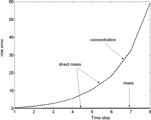
First we regard the scenario with two condensing components. To obtain the single-moment error, we estimate the mass distribution using Equation (8a) with f = 1 and obtain the number distribution using Equation (9b). These errors as a function of time step for the fine–grid evaporation scenario are shown in Figure 1. As expected, the error for the number distribution calculated from the mass distribution (dashed line) is much higher than that for mass distribution (solid line). To emphasize that number is recalculated from mass we designate these curves everywhere as “direct mass.”

FIG. 1 Mass and number r.m.s. errors in the “direct mass” algorithm for condensation scenario on the fine grid.

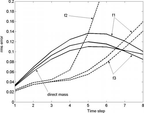
The analogous results when using functions f ₁ through f ₃ in Equation 10 are presented in Figure 2. Solid lines in all figures represent mass distribution errors and dashed lines represent number distribution errors. One can see that functions f ₁ and f ₃ improve the result dramatically, reducing the number error more than 20 times. Function f ₂ did not perform as well, but the result was still better than in the single-moment algorithm.

FIG. 2 Mass and number r.m.s. errors when using functions f ₁ through f ₃ for condensation scenario on the fine grid.

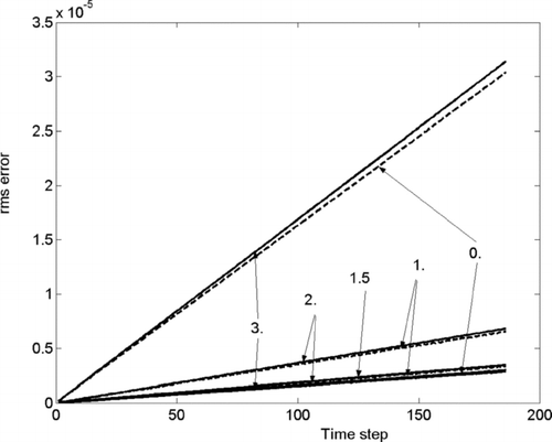
To check the dependence of the error on the choice of μ₀, we performed several runs of the first scenario with f ₁, varying μ₀ between number and mass median diameters: μ₀ = ln D _n + a · ln σ, a = 0, 1, 1.5, 2, 3. Figure 3 shows that as μ₀ moves from ln D _n (number median diameter) to μ₀ = ln D _n + 3.ln σ (mass median diameter), the number error decreases and mass error increases. The best result, when both errors coincide, occurs when μ₀ lies between the limiting cases (μ₀ = ln D _n + 1.5ln σ). This result is quite natural since this intermediate μ₀ equalizes the heights of initial number and mass distributions, thus equalizing also numerical diffusion in both distributions during the calculation. In other words, since numerical error in Equation (8a) comes only from the advection term [q _0,i ^B ] _j ^{n + 1}, mass and number errors are similar when both distributions are equally represented in q _0,i .

FIG. 3 The dependence of errors on the choice of parameter μ₀ = ln D _n + a · ln σ (a = 0, 1, 1.5, 2, 3). The test is run for condensation scenario on the fine grid.

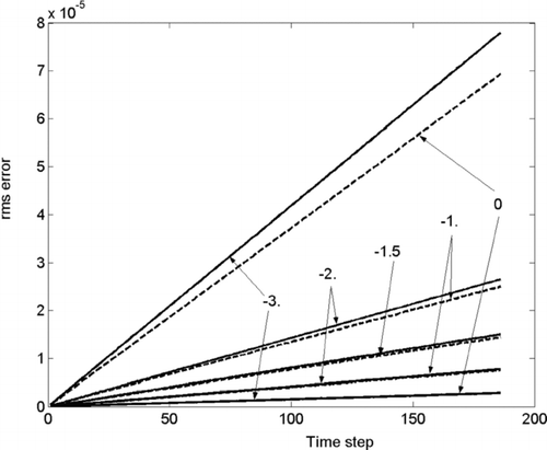
How does the exponent in function f ₂ influence the fine grid results? We changed the power from 0 (3rd moment, mass) to −3 (0th moment, number) (Figure 4). As the power decreases mass error increases and number error decreases, such that for the power –3, mass error is maximal and number error minimal. At the intermediate power –1.5, mass and number errors are similar, but still higher than for f ₁. The main conclusion that we draw from these results is that any intermediate moment provides worse result than the sum of moments (f ₁ or f ₃).

FIG. 4 The dependence of errors on the power in the f ₂ = exp (α · μ) (α = 0, −1, −1.5, −2, −3). Condensation scenario on the fine grid.

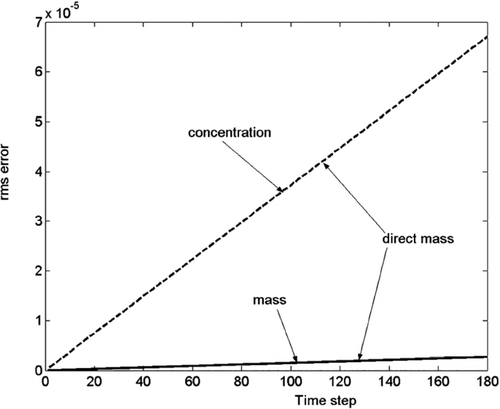
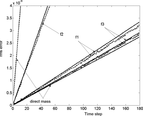
The results for condensing components on the coarse grid are shown in Figures 5 and 6. The number error, when using functions f ₁ and f ₃, is several hundred (!) times less than that in the “direct” method. f ₂ again does not perform as well, but still much better than the “direct” method.

FIG. 5 The same as in Figure 1 for the coarse grid.

FIG. 6 The same as in Figure 2 for the coarse grid.

The errors in the second scenario (condensation/evaporation case) on both grid types turned out to be exactly the same and therefore are not shown. This is natural since again numerical error comes from the advection term [q _0,i ^B ] _j ^{n + 1} and it is the same in both scenarios. This shows that the accuracy of AMDE does not depend on the evaporation or condensation scenario.

Finally, we examined the case with f ₁ varying with time for the second scenario. Errors coincided with those with stationary f ₁ for the same reason, mentioned in the previous paragraph.

We want to emphasize that function f ₃ provided slightly better result than f ₁, illustrating that the smoothing by means of an intermediate moment reduces numerical error.

SUMMARY

Most atmospheric particle dynamic models simulate one moment, typically mass or number. Substantial errors are introduced in these models moving from mass to number or vice versa, since these moments are related by the cube of the particle diameter. Analogous problems may emerge when an application requires prediction of non-integer or intermediate moments. Under the existing practice of working with mass or number distributions, calculating the non-integer moment from available integer ones may also introduce significant errors.

An alternative two-moment aerosol sectional (TOMAS) model, proposed by Adams and Seinfeld (2002), solves the aforementioned problem by estimating both the mass and number distributions simultaneously. This method provides good accuracy for both moments, but requires the solution of two equations and storage of both moments.

In this article we derive the Arbitrary Moment Dynamic Equation that simulates the evolution of an internally mixed multi-component aerosol population distribution due to condensation/evaporation. The equation predicts an arbitrary function of aerosol particle diameter. In other words, it may describe arbitrary distribution moments (both integer and non-integer), as well as an arbitrary linear combination of such moments. For example, simulating the sum of the number and mass distributions allows obtaining both these distributions at the end of simulation from a single function while minimizing moment transformation errors. Another useful application may be found when the non-integer moments are necessary, such as may be encountered when dealing with radiative properties of aerosols.

Important feature of the algorithm proposed is also that instead of a commonly used operator splitting technique (Yanenko 1971; Oran and Boris 1987) we employed real analytical solution of the Equation (2a). This allowed reducing numerical error two orders of magnitude comparing with the algorithm (7).

To test our approach we simulated two scenarios for the two component case: condensation scenario (both components condense) and mixed scenario (one component condenses, another evaporates). The simulations were performed on fine and coarse grids. Three f functions, determining three different distribution functions, q _i , were tested: the sum of the 3rd (mass) and 0th (number) moments; an intermediate 1.5th moment; the sum of all the three moments.

For all the cases we compared the accuracy (normalized difference between numerical and analytical results) in the number distribution estimated from the mass and from q _i distributions. We also compared accuracy for mass distribution when calculated directly and from q _i . Mass errors were found to be similar in all the cases. However, tremendous error reductions were observed for number distribution when using distribution functions that represent the sum of moments proportional to mass and number or when an intermediate smoothing function was added to these. Both these functions reduced the error more than 20 times (fine grid) and several hundred times (coarse grid). The results were identical in both the condensation and mixed scenarios showing that AMDE accuracy does not depend on the concrete scenario.

In summary, when multiple moments (such as mass and number) are needed, their sum provides better accuracy then any intermediate moment. Also the use of an intermediate moment as a smoothing component further reduces error. Thus the best result was obtained when all the three moments were summed. The errors from different moments become similar when the heights of their initial profiles were set equal. This may be gained by adjusting correspondingly parameters μ₀ in f function.

The test with the function f ₁ varying in time shows that AMDE may be applied for tracking particles population when their evolution spans a wide range of particle sizes, as is necessary for cloud modeling.

As a whole, employing an analytical solution of the equation, instead of using operator splitting, together with combining mass and number distributions in one function resulted in an number error reduction by three orders of magnitude.

An important feature of the AMDE is that it may be solved by an arbitrary advection numerical scheme. In this work Bott's positive-definite scheme was employed, but other schemes, like accurate space derivatives (Wexler et al. 1994) or finite elements (Pilinis 1990), could be used as well. Advection schemes (whether they are employed to calculate spatial advection by wind or advection in particle-size space by condensation) are inherently error prone (Rood 1987) and are a primary source of error when calculating the evolution of particle size distributions. The advection error is related to gradients in the concentration over the particle size coordinate. This is the primary reason for the dramatic reduction in error associated with AMDE—the proposed functions f ₁ and f ₃ substantially reduce gradients in the distribution reducing advection error. They also more directly calculate number where it is important (for small particles) and mass where it is important (larger ones).

This work was supported by the California Air Resources Board.

REFERENCES

- Adams , P. J. and Seinfeld , J. H. 2002 . Predicting Global Aerosol Size Distributions in General Circulation Models . J. Geophys. Res. , 107 : D19
- Bott , A. 1989 . A Positive Definite Advection Scheme Obtained by Nonlinear Renormalization of the Advective Fluxes . Monthly Weath. Rev. , 117 : 1006
- Dhaniyala , S. and Wexler , A. S. 1996 . Numerical Schemes to Model Condensation and Evaporation of Aerosols . Atmos. Environ. , 30 : 919 – 928 .
- Gelbard , F. and Seinfeld , J. H. 1980 . Simulation of Multicomponent Aerosol Dynamics . J. Coll. Interface Sci. , 78 : 485 – 501 .
- Intergovernmental Panel on Climate Change (IPCC) . 2001 . “ Third Assessment Report ” . New York : Cambridge University Press .
- Oberdorster , G. 2001 . Pulmonary, Effects of Inhaled Ultrafine Particles International . Arch. Occupat. Environ. Health , 74 : 1 – 8 .
- Oran , S. E. and Jay , Boris P . 1987 . Numerical Simulation of Reactive Flow , Amsterdam : Elsevier .
- Peters , A. , Wichmann , H. E. , Tuch , T. , Heinrich , J. and Heyder , J. 1997 . Respiratory Effects are Associated with the Number of Ultrafine Particles . Amer. J. Respir. Crit. Care Med. , 155 : 1376 – 1383 .
- Pilinis , C. 1990 . Derivation and Numerical Solution of the Species Mass Distribution Equations for Multicomponent Particulate Systems . Atmos. Environ. , 24A : 1923 – 1928 .
- Rood , R. B. 1987 . Numerical Advection Algorithms and their Role in Atmospheric Transport and Chemistry Models . Rev. Geophys. , 25 : 71 – 100 .
- Seinfeld , J. H. and Pandis , S. N. 2006 . Atmospheric Chemistry and Physics, , 2nd , New York : Wiley & Sons .
- Yanenko , N. N. 1971 . The Method of Fractional Steps , Berlin : Springer .
- Zhang , K. M. and Wexler , A. S. 2002 . Modeling the Number Distributions of Urban and Regional Aerosols: Theoretical Foundations . Atmos. Environ. , 36 : 1863 – 1874 .
- Wexler , A. S. , Lurmann , F. W. and Seinfeld , J. H. 1994 . Modelling Urban and Regional Aerosols—I. Model Development. . Atmos. Environ. , 28 : 531 – 546 .