Inversion of Andersen Cascade Impactor Data using the Maximum Entropy Method

Abstract

The problem of the Andersen cascade impactor data inversion is studied using the maximum entropy method to recover the particle size distribution function from a set of measured masses collected on the impactor stages. The classical entropy maximization and its modification to accommodate data errors are reviewed using the techniques of convex optimization. Numerical experiments were performed to test the method on several unimodal and multimodal distributions commonly observed in practice. The Maximum Entropy Method for data inversion produced excellent agreement between the recovered and test Particle Size Distribution Functions without the need for a priori assumptions.

1. MOTIVATION AND PROBLEM STATEMENT

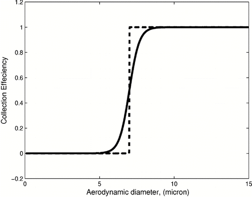
One of the major purposes of the Andersen cascade impactor (ACI) is to determine the particle size distribution of the particles suspended in the air flowing through the device. Cascade impactors consist of a number of stages in series each of which is designed to retain particles about a particular size. As the aerosol of interest is convected through the device, the particle size that each consecutive stage is designed to retain is decreased. The probability that a particle of a certain size will impact on a particular stages is known as the stages collection efficiency curve. Traditionally, cascade impactor stages have been designed to achieve a maximally steep efficiency curves. However, in practice curves take on a sigmoidal type shape (Figure 1). After enough material is collected the amount retained on each can be determined by weight or chemical assay and then the particle size distribution function (PSDF) can be recovered using the measured data. The PSDF recovery, usually regarded as the impactor data inversion is, in general, mathematically ill posed—there are many possible distributions consistent with the observed masses (Fuchs 1978).

FIG. 1 Ideal (dashed) vs. non-ideal (solid) efficiency curves, both with a D50 at 5 microns.

If an impactor did have maximally sharp efficiency curves it would allow for a simplified data inversion (Andersen 1958; Marple and Willeke 1976). In practice, an estimation of an ideal efficiency curve can be associated with a 50% probability of impaction (d ₅₀) for each curve (Figure 1). Indeed, assuming the ideally sharp cuts at 50% cut points (d ₅₀), the resulting probability distribution can be obtained by dividing the mass fraction g _i = m _i /M, M = ∑ _{j = 0} ⁷ m _i of the collected particles on the stage i by the particle size interval:

This distribution is a piecewise constant function and usually presented as a histogram; the corresponding smooth distribution can be approximated by drawing a curve through the mid-points of the size intervals.

In practice, the accuracy of this simplified approach is compromised because multiple size ranges get collected on a single impactor stage. Consequently more complex distributions, such as multimodal ones, can be completed missed. The collection efficiency curves are typically S-shaped and show a large degree of overlap. While such overlaps make the simplistic inversion approach mentioned above more inaccurate, they provide additional information about the distribution that if properly taken into account, can help recover the most “realistic” distribution, consistent with the measured masses.

A formal description of the inverse problem can be given as follows. Assuming that a set of S-shaped efficiency curves S _i (d) for stages i = 0,1,…,7 is available from the impactor calibration, the PSDF P(d) sought is a solution of the first-kind Fredholm integral equation with a discrete right hand side

where d is the particle aerodynamic diameter, a and b are the size limits within which the distribution lies, and ε _i is the instrumental error of the stage (Rader 1991). The stage response (or kernel) functions R _i (d), which are given by the relations:

are shown in Figure 2 along with the corresponding stage efficiency curves based on the least-square fit of the manufacturer's calibration data (Vaughn 1989).

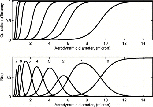
FIG. 2 Collection efficiency data (top) and corresponding stage response functions (bottom) for stages 0 to 7 (right to left).

Problem (2) is a classical case of an underdetermined ill-posed problem. A number of techniques have been developed to recover the distribution from Equation (2). One group of methods is based on an a priori assumption about the functional form of the distribution, for instance a superposition of log-normal and normal, with further determination of the coefficients of the assumed form. The disadvantage of this approach is that the parametric form of the PSDF is not usually known; in fact, it is the very thing that we seek to determine.

In more recent years, several non-parametric regularization methods have been proposed to overcome the ill-posedness of the data inversion problem. The idea of regularization is to incorporate some additional information about the solution in order to compute a unique and stable solution. Thus, the well-known Tikhonov regularization scheme (Hansen 1998) reduces to a minimization of the residual with an additional “smoothing” constraint Ω (P) ≥ 0

which is typically proportional to the second derivative of the solution. Here the regularization parameter γ controls the balance between the allowable residual error and the smoothness of the resulting distribution. Thus, an optimal choice for the parameter γ is an important step of the algorithm; it can be determined using the L-curve method (Hansen 1998).

Besides the Tikhonov regularization, there are many other inversion techniques that have been used in aerosol science to determine the aerosol PSDF. A critical survey and comparison of several popular methods is presented in Kandlikar and Ramachandran (1999), which includes constrained least squares, truncated singular value decomposition, Twomey's nonlinear approach, and Bayesian methods. The conclusion of the survey indicates that there is no single algorithm that can be considered superior to others, and applicable for all types of aerosol spectrometers such as impactors, elutrilators, nephelometers, and diffusion batteries. Also, while different algorithms produce PSDF that match the experimental data well, the resulting distributions may be quite different from each other.

In the present work, we examine the ACI data inversion problem using a maximum entropy method, which was originally proposed by Janes (1957) as a variational technique to calculate equilibrium states in statistical physics, as well as for solving inverse problems (Janes 1984). This method has proven in many other disciplines to be useful and efficient for recovering probability distributions from information on a few of its moments (Kapur 1989). In the field of aerosol spectrometry, the entropy maximization was introduced two decades ago in Yee (1989) to reconstruct the PSDF from diffusion battery measurements, but to our knowledge, has not been applied to the inversion of the ACI data since then.

From a technical viewpoint, one of the advantages of the maximum entropy method is that it can be considered as a special case of the convex optimization problem, which allows us to rely on general existence and duality theory for this problem (Borwein and Zhu 2005) and also simplifies its computational treatment. However, since the aim of this article is to describe a reliable and efficient data inversion procedure with a particular application in mind, we provide only formal (heuristic) derivations that lead directly to computational schemes. Other interesting details on the rigorous problem formulations, solution functional spaces, the analysis and proofs of the existence, and characterization of the maximum entropy solution can be found in Hiriart-Urruty and Lemaréchal (1993), Borwein and Zhu (2005), and references therein.

The structure of the article is the following. In Section 2, we first discuss a classical maximum entropy maximization (the primal problem) using Lagrange multipliers. Then, exploiting the convexity of the original problem, an alternative computational scheme based on dual formulation is described. As a result, the original infinite-dimensional problem reduces to a solution of finite dimensional nonlinear system in the former case, or to the maximization of a dual function of finitely many variables in the latter case. Section 3 presents a modification of primal-dual computational models that allows imprecise data values in the constraints. Section 4 gives details of the algorithmic implementation and computational results.

2. MAXIMUM ENTROPY METHOD

The basic idea of the maximum entropy approach to obtain a unique and robust particle size distribution P(d) from the data g _i is to maximize the Boltzmann-Shannon-Jaynes entropy

under the constraints represented by Equation (2) and a normalization condition:

where instrumental errors ε _i are initially neglected. The entropy is employed here as a measure that allows one to choose the “most probable” or “maximally noncommittal with regard to missing information” (Jaynes 1957) distribution among other distributions, having a substantially lower entropies than the maximal one. The entropy maximization (5)–(7) is a constrained optimization problem which can be put into the standard form as follows (note: for the sake of readability the symbol “x” has replaced the variable for “d”):

and is equivalent to the maximization of the entropy − H; the linear term is included into the entropy expression mostly for convenience. This is a primal problem, which is traditionally approached using the method of Lagrange's multipliers to recover the PSDF. We first define the Lagrangian by augmenting the objective functional with the linear combination of the constraints

where vector λ and scalar ν are the Lagrange multipliers. As a result, minimizing the Lagrangian by computing the variation of L(P;λ,ν) with respect to P gives

The multiplier ν can be eliminated using the normalization constraint in Equation (8) and the resulting PSDF has the form

Now, the unknown multipliers λ _i , i = 0, …,7 can be found as solutions of a nonlinear system obtained by substituting this expression for P(x) into the remaining constraints in Equation (8). This gives a nonlinear system of 8 equations for 8 unknowns

that, in principle, can be solved numerically. Note that the maximum entropy PSDF (Equation (11)) is an explicit nonlinear combination of the impactor response functions.

While the formal derivation above usually leads to the solution, an alternative approach that uses convex duality is often preferred. It allows detailed, rigorous analysis of the maximum entropy solution and, in certain cases, dual problems are easier to solve numerically. To illustrate the basic idea of the duality, we define the (Lagrange) dual function as the minimum value of the Lagrangian (Equation (9)) over P

The optimization problem in λ, ν

is a dual problem associated with Equation (8). By denoting the optimal value of H in Equation (8) as p and letting d = sup_λ,ν D(λ,ν), it is not difficult to show that the weak duality inequalityp ≥ d is always satisfied: the optimal value of the dual problem gives an upper bound on the primal optimal value. Due to the special properties of the entropy maximization, however, it can be shown that for this problem the strong duality p = d holds. In particular, these properties are the strict convexity of the entropy Plog P − P as a function of P, and the affinity of constraints in Equation (8). See Hiriart-Urruty and Lemaréchal (1993) and Borwein and Zhu (2005) for further details and discussion of possible technical difficulties. From a practical viewpoint, the crucial importance of strong duality is that it allows to obtain a primal optimal solution from a dual optimal solution. Thus, if λ and ν solve the dual problem (Equation (14)), substituting these values of λ into (Equation (11)) gives the solution to the primal problem.

To obtain a practical formulation of the dual problem (Equation (14)), the dual function has to be evaluated by minimizing the Lagrangian (Equation (9))

The last expression can be simplified using the formula

where h ^☆ (y) = sup _z {yz − h(z)} is a convex (Fenchel) conjugate of a function h (Borwein and Zhu 2005). Since the conjugate of zlog z − z is exp y and

this finally gives

Thus, the dual problem is the unconstrained maximization of the expression (18) with respect to λ and ν

It can be further simplified by maximizing over ν for fixed λ, which results in

Substituting this value of ν into Equation (19) gives the final form of the dual problem

with respect to λ. The resulting PSDF is obtained by substituting these λs into the expression (11). Note, that the dual formulation (Equation (21)) is not only more elegant than the reduction of the primal problem to the nonlinear system, but also provides an alternative numerical pathway for the entropy maximization treatment.

3. MAXIMUM ENTROPY WITH NOISY DATA

One problem with the analysis presented above is that the stage loadings g _i , in most practical applications, cannot be determined precisely since all measurements will have some level of uncertainty. A classical way to account for such errors is to apply a χ² statistic to define a confidence region about the expected value, assuming that the observation noise is Gaussian. In the frame of the maximum entropy method, this can be accomplished by replacing exact constraints on the stage loadings g _i in Equation (8) by a single constraint (Skilling and Bryan 1984; Yee 1989)

where σ _i is the standard deviation associated with the stage loadings g _i , and M is usually taken as a number of measurements, i.e., the number of impactor stages. A modified primal problem can be now written as

This problem can be reformulated by introducing new variables ξ _i = ∫ ^b _a P(x)R _i (x)dx− g _i ,    i = 0, 1, …, 7 and associated equality constraints:

whose Lagrangian is

Here L(P;λ,ν) is the Lagrangian (Equation (9)) of the problem with the exact constraints. Note, that [Ltilde] can be minimized separately with respect to P and ξ. The variation of [Ltilde] with respect to P gives the same expression (11) for the PSDF (however, with different values of λ _i ), and with respect to ξ:

The value of μ can be found by substituting Equation (26) into the second constraint of Equation (24). Finally, putting the resulting expressions for the ξ _i and the PSDF (Equation (11)) into the first constraint of Equation (24) produces a system of 8 nonlinear equations for the unknowns λ _i , i = 0,1,…,7:

To find the dual function for the problem (Equation (24)) we minimize [Ltilde] over P and ξ, which can also be done separately:

The dual problem now reduces to the maximization of the last expression with respect to λ, ν, and μ. The maximization in μ can be carried out explicitly, and using the result of Equation (21) the final form of the dual problem is an unconstrained maximization with respect to λ:

4. IMPLEMENTATION AND RESULTS OF COMPUTATIONS

As follows from the above discussion, the infinite-dimensional constrained entropy maximization can be reduced to the solution of the finite (low) dimensional nonlinear system (primal problem) or unconstrained minimization (dual problem). These finite-dimensional problems can be solved directly using standard numerical analysis techniques, such as the Newton's method. We implemented both the primal and dual problems in Matlab (The MathWorks Inc., Natick, MA) utilizing the Optimization toolbox that provides standard routines for the unconstraint minimization and nonlinear system solvers. We also employed an excellent, recently developed Chebfun system (Trefethen et al. 2008), which allows practically symbolic manipulation of Matlab data and functions. This system is particularly convenient for handling recursive computations with the impactor stage response functions internally represented as Chebyshev polynomials.

To test how well different PSDF can be reconstructed using the maximum entropy approach, our computational experiments were performed in the following sequence:

1.	assume some initial distribution P(d), such as log-normal, Rosin-Rammler, etc.;
2.	calculate the corresponding stage loadings g i = ∫ a b P(d) R i (d) d(d), i = 0,1,…,7 where the particle size limits are taken as a = 0.2, b = 15;
3.	perform the inversion and compare with the initial distribution.

Note that in step 2, we initially assume accurate measurements of the stage loadings without adding noise to the data.

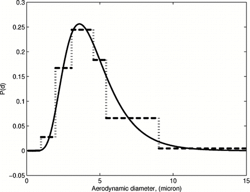
In our first test case, we use the ideal, piecewise constant collection efficiency/response functions to recover a log-normal initial distribution. Figure 3 shows the initial (smooth line), as well as the resulting PSDF (dashed line), which is also a piecewise constant function. This result can be confirmed analytically in this case, and the maximal entropy solution is identical to Equation (1). This test illustrates both the strength and the weakness of the entropy maximization method. Indeed, the recovered distribution is not smooth; however, as often argued, it is the one most objectively consistent with the incomplete available information.

FIG. 3 Log-normal distribution recovered using the ideal efficiency/response data; solid curve: incoming distribution, dashed curve: recovered distribution.

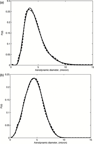
In further tests, we use the manufacturer's calibrated efficiency/response data shown on Figure 2. We experiment next with the log-normal and the Rosin-Rammler initial distributions. The Rosin-Rammler (also known as Weibull) distribution has a density function

where λ and k are the scale and shape parameters, respectively. Figure 4 demonstrates good agreement between the resulting curves and initial distributions, as well the much higher resolution obtained with the smooth and overlapping impactor response functions in comparison with the ideal ones.

FIG. 4 Maximum entropy inversion of the log-normal (top) and Rosin-Rammler (bottom) distributions; solid curve: incoming distribution, dashed curve: recovered distribution.

Next, we consider more complicated multimodal initial distributions. The bimodal distribution is a superposition of two log-normal distributions. The trimodal consists of two log-normal and one normal distribution. Figure 5 shows that the bimodal distribution is recovered quite satisfactorily, giving reasonable estimates of the distribution peak positions. However, two peaks of the trimodal distribution on the interval between 6 and 10 micron have not been properly resolved, which reveals that the resolution quality of the PSDF might not be uniform on the considered particle size interval. To examine this issue, we define a bimodal distribution and translate it along the d axis from left to right, applying the maximum entropy method at several intermediate points. The results are presented in Figure 6 and demonstrate the loss of resolution and larger shifts of the distribution peaks as the original distribution moves to the right.

FIG. 5 Maximum entropy inversion of the bimodal superposition of two log-normal (top) and trimodal superposition of two log-normal and one normal distributions (bottom); solid curve: incoming distribution, dashed curve: recovered distribution.

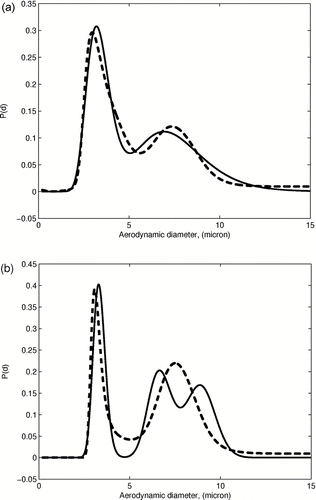
FIG. 6 Demonstration of the effect of spatial nonuniformity of the response functions. As the incoming biomodal (solid line) is shifted to the right the quality of the recovered distribution (dashed line) is at first slightly improved and then it degenerates. This is caused by the shape and spacing variability in the impactors response functions.

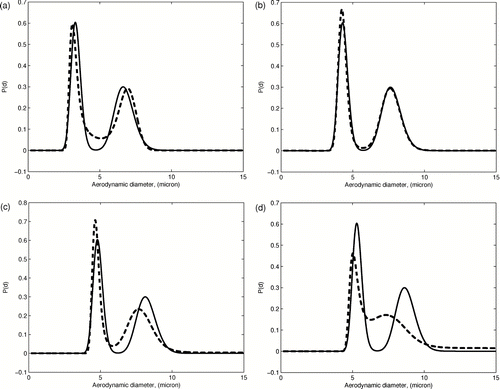
On the last graph of Figure 6, the second peak cannot be identified at all, which corresponds to a 2 micron translation of the original PSDF, which appeared on the first graph.

The observed resolution problem can be understood by analyzing the approximation properties of the maximum entropy solution (Equation (11)), which indicates that the logarithm of the PSDF is approximated by a linear combination of the impactor stage response functions. The response functions, however, are not evenly distributed on the considered particle size interval, as shown on Figure 2. Clearly, a larger gap between them can be seen on the interval from 6 and 10 micron, which results in a growth of the PSDF approximation error on this interval.

The consequences of this observation are clear: if the maximum entropy method is to be used to invert the distribution, then instead of minimizing overlap between S-curves, one needs uniform overlap between S-curves.

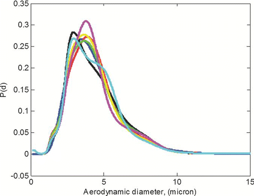
In the next test we perform the reconstruction of the PSDF from the stage loadings data that contains random measurement errors. Such errors can be simulated by adding noise to the calculated exact values of the stage loadings g _i obtained on step 2 of our numerical procedure. To examine the sensitivity of the inversion, we used the stage loadings calculated for the initial log-normal distribution shown on Figure 3, superimposed with the up to 10% uniformly distributed random noise. However, we assume that the thus obtained values of g _i represent accurate stage loading measurements. Figure 7 shows several PSDF recovered from the corresponding noisy data sets. The perturbation of the stage loadings clearly affects the recovered distributions, but does not produce high-frequency instabilities and preserves the shape of the original PSDF. We noticed, however, a slower convergence of the nonlinear system, as well as the minimization solvers in the course of these computations.

FIG. 7 Recovery of noisy data stage loadings with up to 10% noise.

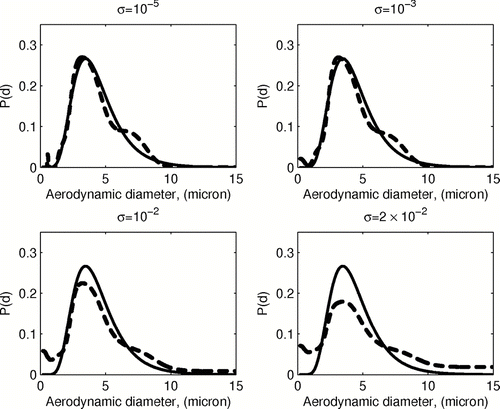
Finally, we performed numerical experiments using the maximum entropy inversion procedures for imprecise data, based on the formulations (27) and (29), assuming the uniform noise level σ _i = σ for all impactor stages. Here we again attempt to reconstruct the log-normal distribution shown on Figure 3 from the data obtained by adding the Gaussian noise (with a mean and standard deviation of 0 and 0.02, respectively) to the theoretically exact stage loadings data. A particular noisy data set, generated this way, is presented in Table 1 along with the corresponding “exact” fractional stage loadings.

TABLE 1 Fractional impactor stage loadings

Stage	0	2	2	3	4	5	6	7
Estimated stage loadings	0.0258	0.1571	0.1723	0.3404	0.2384	0.0649	0.0011	0.0000
Stage loadings with noise	0.0194	0.1868	0.1548	0.3211	0.2478	0.0665	0.0016	0.0019

For this noisy loadings data, the classical maximum entropy approach fails to converge. Figure 8 shows the PSDF, recovered using different values of the noise level σ. Choosing large values of the parameter σ results in over-smoothing of the distribution; however, reasonably accurate recovery can be achieved even by taking σ smaller that the actual noise level.

FIG. 8 Recovery of noisy data using different values of the noise level σ: solid line shows the original distribution without added noise.

5. SUMMARY

The results of our study show that the maximum entropy method is an accurate and reliable technique of reconstructing the aerosol PSDF from the ACI measurements. The method performed well on the distributions commonly observed in practice, such as log-normal, Rosin-Rammler, and bimodal distributions. The main advantages of the entropy maximization are the following:

•	The method inverts Cascade Impactor data using no a priori assumption about the shape of the distribution.
•	The method is based on sound physical and information theory principles, in contrast with many other regularization techniques.
•	The mathematical theory of the entropy maximization is well developed and allows to transform the original infinite-dimensional problem into a finite dimensional one.
•	The numerical implementation of the method reduces to readily available, efficient algorithms.

Using the maximum entropy, we observed that the accuracy of the inversion crucially depends on the shape and the spatial position of the collection efficiency/response curves. In addition, the maximum entropy technique performs best when a certain degree of overlap exists between neighboring stages. Since most Cascade Impactors still have a significant deal of overlap between the stages, this technique may be appropriate to extend the utility of their data. We also observed that the spatial distribution of the efficiency curves strongly affects the quality of the inversion. The study of this relationship, however, requires further work and will be reported elsewhere.

REFERENCES

- Andersen , A. A. 1958 . New Sampler for the Collecting, Sizing, and Enumeration of Viable Airborne Particles . J. Bacteriol. , 76 ( 5 ) : 471 – 484 .
- Borwein , J. and Zhu , Q. J. 2005 . Techniques of Variational Analysis , Springer .
- Fuchs , N. A. 1978 . “ Aerosol Impactors: A Review ” . In Fundamentals of Aerosol Science , Edited by: Shaw , D. T. 1 – 83 . New York : Wiley & Sons .
- Hansen , P. C. 1998 . Rank-Deficient and Discrete Ill-Posed Problems: Numerical Aspects of Linear Inversion , Philadelphia : SIAM .
- Hiriart-Urruty , J.-B. and Lemaréchal , C. 1993 . Convex Analysis and Minimization Algorithms. II , Berlin : Springer-Verlag .
- Jaynes , E. T. 1957 . Information Theory and Statistical Physics . Phys. Rev. , 106 : 620 – 630 .
- Jaynes , E. T. 1984 . “ Prior Information and Ambiguity in Inverse Problems ” . In Inverse Problems , Edited by: McLaughlin , D. W. Providence, RI : Am. Math. Soc. .
- Kandlikar , M. and Ramachandran , G. 1999 . Inverse Methods for Analyzing Aerosol Spectrometer Measurements: A Critical Review . J. Aerosol Sci. , 30 : 413 – 437 .
- Kapur , J. N. 1989 . Maximum-Entropy Models in Science and Engineering , New York : John Wiley & Sons .
- Marple , V. A. and Willeke , K. 1976 . Impactor Design . Atmos. Environ. , 10 : 891 – 896 .
- Rader , D. J. , Mondy , L. A. , Brockmann , J. E. , Lucero , D. A. and Rubow , K. L. 1991 . Aero. Sci. Tech. , 14 : 365 – 379 .
- Skilling , J. and Bryan , R. K. 1984 . Maximum Entropy Reconstruction: General Algorithm . Mon. Not. R. Astr. Soc. , 211 : 111 – 124 .
- Trefethen , L. N. , Pachón , R. , Platte , R. B. and Driscoll , T. A. 2008 . Chebfun Version 2 , Oxford University . http://www.comlab.ox.uk/chebfun
- Vaughn , N. P. 1989 . The Andersen Cascade Impactor: Calibration, Wall Loses and Numerical Simulation . J. Aerosol Sci. , 20 : 213 – 221 .
- Yee , E. 1989 . On the Interpretation of Diffusion Battery Data . J. Aerosol Sci. , 20 ( 7 ) : 797 – 811 .