Feasibility of the Detection of Trace Elements in Particulate Matter Using Online High-Resolution Aerosol Mass Spectrometry

Abstract

The feasibility of using an online thermal-desorption electron-ionization high-resolution aerosol mass spectrometer (HR-AMS) for the detection of particulate trace elements was investigated by analyzing data from Mexico City obtained during the MILAGRO 2006 field campaign. This potential application is of interest due to the real-time data provided by the AMS, its high sensitivity and time resolution, and the widespread availability and use of this instrument. High-resolution mass spectral analysis, isotopic ratios, and ratios of different ions containing the same elements are used to constrain the chemical identity of the measured ions. The detection of Cu, Zn, As, Se, Sn, and Sb is reported. There was no convincing evidence for the detection of other trace elements commonly reported in ambient particulate matter (PM). The elements detected tend to be those with lower melting and boiling points, as expected given the use of a vaporizer at 600°C in this instrument. The detection limit (DL) is estimated at approximately 0.3 ng m⁻³ for 5 min of data averaging. Concentration time series obtained from the AMS data were compared to concentration records determined from offline analysis of particle samples from the same times and locations by inductively coupled plasma based techniques (ICP; PM_2.5) and proton-induced X-ray emission (PIXE; PM_1.1 and PM_0.3). The degree of correlation and agreement between the three instruments (AMS, ICP, and PIXE) varied depending on the element. The AMS shows promise for real-time detection of some trace elements, although additional work including laboratory calibrations with different chemical forms of these elements is needed to further develop this technique and to understand the differences with the ambient data from the other techniques. The trace elements peaked in the morning as expected for primary sources, and the many detected plumes suggest the presence of multiple point sources, probably industrial, in Mexico City, which are variable in time and space, in agreement with previous studies.

Copyright 2012 American Association for Aerosol Research

1. INTRODUCTION

The mass concentration of ambient fine particles is usually dominated by sulfates, nitrates, organic compounds, and black carbon (composed mainly of C, H, O, S, and N). However, they also contain a wide spectrum of other trace elements with concentrations typically of the order of ng m⁻³. Emissions of trace elements to the environment occur through a wide range of processes, and impact air, water, and soil. Airborne emissions are of particular concern because of the toxicity of some of the chemical forms of these elements and the potential for high dispersion and exposure of emissions to the atmosphere (Järup 2003; Wong et al. 2006). Trace elements are usually emitted to the atmosphere in the condensed phase (particulate matter, PM) due to the low vapor pressure of the chemical compounds that they form. There is strong evidence that associates high concentrations of fine PM with adverse health effects (Pope and Dockery 2006). Because the chemical composition of PM is highly variable by geographical location, it needs to be considered, along with size and total mass concentration, as a variable influencing health effects. However, there is still uncertainty as to which particle chemical components are most harmful (Franklin et al. 2008; Lippmann 2009).

Growing applications of trace elements in the production of new materials have amplified their sources to the urban environment. Furthermore, there is increasing evidence of negative health effects of some of them (Wong et al. 2006). Hence, chemical analysis of airborne particles, which includes trace element composition, has become an important aspect of atmospheric and health effects related studies. In addition, elemental analysis of PM is important because it can be very helpful in identifying particle sources and their contribution to fine mass atmospheric concentration (Lippmann 2009).

Lead (Pb) continues to be one of the most studied contaminants in the urban environment, including the atmosphere. However, with the reduction in Pb emissions to the atmosphere due to the decline in the use of leaded gasoline in many countries, interest has increased on other potential toxic trace elements such as Cd, Hg, Zn, Cu, and Ni, which are among the most commercially used and emitted (Wong et al. 2006; Charlesworth et al. 2011). For example, among the 187 hazardous air that the U.S. Environmental Protection Agency (EPA) is required to control, there are several trace elements (Sb, As, Be, Cr, Co, Pb, Mn, Hg, Ni, and Se) and their compounds (http://www.epa.gov/ttn/atw/orig189.html). The EPA program “National PM_2.5 Chemical Speciation Monitoring Network (CSN)” (http://www.epa.gov/ttnamti1/specgen.html) includes the monitoring of the following elements: Al, Si, K, Ca, Ti, V, Cr, Mn, Fe, Ni, Cu, Zn, As, Se, Br, Cd, and Pb (EPA 1999). The United Nations Environmental Program (UNEP) includes Pb, Sn, and Hg in the list of Persistent Toxic Pollutants, which need to be monitored (http://www.chem.unep.ch/pts/). Finally, the European Union (EU) has set air quality standards (which will enter into force as on 31/12/2012) for As, Cd, and Ni (6, 5, and 20 ng m⁻³, respectively) (EP 2008).

Several studies have analyzed data or samples from the MILAGRO field experiment in March 2006 in Mexico City focusing on trace elements content in PM. A diversity of concentrations and associations were identified, which were time- and site-dependent and suggested mainly traffic, crustal, and unidentified industrial sources. Querol et al. (2008) and Mugica et al. (2009) reported relatively high concentrations of several trace elements at several sites within the Mexico City Metropolitan Area (MCMA). Typically, anthropogenic elements (As, Cr, Zn, Cu, Pb, Sb, and Ba) showed considerably high levels at urban sites; while levels of particulate Hg and crustal trace elements (Rb, Ti, La, Sc, and Ga) were generally higher at suburban sites (Querol et al. 2008). Moreno et al. (2008), using scanning electron microscope/energy-dispersive X-ray spectroscopy (SEM/EDX) microanalysis found that metals such as Fe, Ti, Ba, Pb, Cu, and Zn, commonly occur alone in particles collected at the main site during MILAGRO (T0); however, Zn-containing particles can also contain Cu, Pb, Sn, or Fe; Cu was detected together with As; and Pb with Sb, and Cr. They also noted a nightly increase in metal PM. Furthermore, Pb, Cu, and Zn show individual element nocturnal concentration spikes, which are not correlated with each other. Adachi and Buseck (2010) used transmission electron microscopy (TEM) to measure size and composition of individual particulate trace elements collected from ambient air above Mexico City during MILAGRO. They found that more than 60% of the analyzed particles contained two or more metals, with Fe, Pb, or Zn being the most abundant. The combination of metals present in individual particles was very variable. Moffet et al. (2008a,b) suggested that particles containing Na, Cl, Zn, and Pb detected at T0 are partly due to refuse and paper burning in Mexico City. In addition, Sb was suggested as a tracer for trash burning in Mexico City (Christian et al. 2010; Hodzic et al. 2012).

Concentrations of trace elements are traditionally monitored with offline techniques, which often suffer from low time resolution and result in long delays between sample collection and data reporting (Baron and Willeke 2001). Trace element concentrations with time resolutions of 1 h have been recently reported (Richard et al. 2010), but these require analysis at synchrotron facilities of limited availability. The Aerodyne High-Resolution Time-of-Flight Aerosol Mass Spectrometer (HR-ToF-AMS) is a widely used online instrument, which has been recently used to determine Pb concentrations in submicron PM (Salcedo et al. 2010). In this article, we investigate the feasibility of detection of other important trace elements with this instrument using several analysis techniques, and compare the results with two offline methods.

2. EXPERIMENTAL

2.1. High-Resolution Aerosol Mass Spectrometer During MILAGRO

The MILAGRO field experiment took place in March 2006 in and around Mexico City with the objective of characterizing the sources, concentrations, transport, and atmospheric aging processes of the gases and fine particles in the MCMA, and to evaluate the regional and global impacts of its atmospheric emissions (Molina et al. 2010). One of the three main ground-sampling sites during MILAGRO was the urban supersite “T0,” located within the northern part of the MCMA in a mixed-use neighborhood (small industries, residential, and commercial), and south of a large area of small industries.

An Aerodyne high-resolution time-of-flight aerosol mass spectrometer (HR-ToF-AMS, referred to as AMS hereafter) (DeCarlo et al. 2006) was deployed at T0 during the MILAGRO campaign. The AMS operation, calibrations, comparisons with collocated instruments, and overview of the results during this period have been already described by Aiken et al. (2008, 2009, 2010) and Salcedo et al. (2010). Briefly, the AMS was located on the roof of a four-story building and sampled continuously from 10–30 March, 2006. During the measurement period, high-resolution aerosol mass spectra (m/z 4–400, representing ensemble averaging of tens of thousands of individual particles) were acquired every 2.5 min, alternating between V and W modes every 5 min. These two modes of operation of the AMS refer to different ion paths in the ToF spectrometer; V-mode is about ten times more sensitive, but W-mode offers about two times higher mass resolution (DeCarlo et al. 2006).

Raw AMS signals have been corrected for small variations in detection sensitivity (i.e., air beam correction, Allan et al. 2003); and converted to “nitrate-equivalent mass concentrations” (Nit.-eq. ng m⁻³, Jimenez et al. 2003). In order to calculate the actual mass concentration of a species other than nitrate, the ionization efficiency of component x relative to nitrate (RIE _x ) is used (Jimenez et al. 2003; Canagaratna et al. 2007). The collection efficiency correction (CE) is also necessary in order to account for detection losses, mainly due to bounce of particles off the vaporizer (Middlebrook et al. 2012):

where C_x is the concentration of component x in ng m⁻³ and C_{x ,Nit.-eq.} is the nitrate-equivalent mass concentration discussed previously.

All AMS signals and mass concentrations reported were calculated using a CE value of 0.5, which is consistent with the submicron chemical composition and has resulted in good agreement with a wide variety of particulate instruments in the MCMA (Salcedo et al. 2006; Kleinman et al. 2008; Aiken et al. 2009; Salcedo et al. 2010). As a first approximation, RIE _x = 1 was chosen and applied to the data shown in this article (as indicated in the axis labels of the figures). The estimation of a more accurate RIE _x for the detected elements is discussed in Section 3.3.

The AMS spectra were analyzed for the presence of features indicative of trace elements containing compounds (Section 3.1). In order to determine the detection limits (DLs) for those elements, five different regions in the mass spectra with a mass defect with respect to nominal m/z's 63, 75, 90, 105, and 124 were chosen. The regions span over a range of the spectra, where all the detected trace element ions are found. In these regions, no signal from a chemical compound was expected, and the observed HR signal did not show any evident trend. Hence, it was assumed that the observed signal was only due to the instrument background and electronic noise. The average signal during the whole campaign plus three times its standard deviation was calculated for V and W modes at each of the chosen m/z values. The five values obtained for each mode were averaged to be reported as the DL for 5 min. This method was chosen for estimating DL because the ions of trace element are generally located in similar regions of the mass spectra, free of interferences from other fragments, and because the level of noise in the high-resolution fittings is typically comparable to the level of noise in the raw spectra. From Section 3.3, where the estimation of RIE _x is discussed, we chose an average value of RIE _x = 0.6 in order to calculate an approximate DL of 0.3 and 1.2 ng m⁻³ in 5 min for V and W modes, respectively. These DLs are better than those typically observed in the AMS for nonrefractory species (DeCarlo et al. 2006) due to the lack of instrument background.

Mass concentrations are reported in ng am⁻³ at local ambient pressure (∼780 mbar) and temperature (ng am⁻³, where the “a” in “am³” indicates that the volume was measured under ambient conditions). These concentrations should be multiplied by ∼1.40 to obtain concentrations under standard temperature and pressure (STP) conditions of 273 K and 1 atm. Time series are reported in local standard time, which is the same as US Central Standard Time (CST), or Coordinated Universal Time (UTC) minus 6 h.

2.2. AMS Vaporizer Model

Within the AMS, a chopper modulates the transmission of the sampled aerosol beam to the particle detector by continually switching between the “closed” and “open” positions (blocks the beam completely, or transmits the beam completely, respectively) every few seconds (3 s in our study). Then, the beam of the sampled ambient particles hits the vaporizer, where particulate species of sufficient volatility evaporate, prior to electron ionization and detection using time-of-flight mass spectrometry (ToFMS) (Canagaratna et al. 2007). During MILAGRO, the vaporizer operated at the standard AMS temperature of ∼600°C.

The standard data analysis procedures of the AMS for “nonrefractory” species rely on the rapid evaporation of the PM components on the vaporizer before entering the mass spectrometer section. For those components that evaporate much faster than the open/close alternation time of the particle-beam blocking device, the closed signal is usually small and represents the instrument background; while the open signal minus the closed (“difference” signal) represents the signal produced by the aerosol entering the instrument (Huffman et al. 2009). However, chemical species that evaporate from the vaporizer on slower time scales than nonrefractory material present significantly larger closed signals. In this case, the difference signal cannot be directly interpreted because the open and closed signals become a combination of the PM entering the instrument and the signal of residual components that slowly evolve from the vaporizer (Salcedo et al. 2010). Species that evaporate in the AMS with such timescales are referred to as “semirefractory.”

As will be discussed later, most trace element compounds found in ambient PM tend to have relatively large closed signals. Hence, the vaporizer model developed by Salcedo et al. (2010) was used to estimate “input” signals (i.e., the actual ambient PM₁ concentrations sampled by the AMS) from the observed open and closed signals. The model assumes that there are two components generating the signals, each one desorbing at a different rate. The components might correspond to different chemical species that result in the same detected ion. Results from the model include the fraction of each component in the aerosol (which is assumed to be constant during the campaign), the evaporation time constant of each component, and the total input signal of the species generating the AMS signals.

TABLE 1 Trace element ions detected in the AMS spectra of ambient particles at T0 during MILAGRO, and their exact m/z and isotopic ratios

Element or compound	Ion	Exact m/z ^a,b	Relative abundance^a	AMS mode detection	Notes
Cu^+	^63Cu^+	62.9296	1	V
	^65Cu^+	64.9278	0.4461
Zn^+	^64Zn^+	63.9291	1	V and W	Interference from SO2 ^+
	^66Zn^+	65.9260	0.5796		Used as main ion
	^67Zn^+	66.9271	0.0850		Unknown interference
	^68Zn^+	67.9248	0.3941
ZnCl^+	^64Zn^35Cl^+	98.8980	1	V and W
	^66Zn^35Cl^+	100.8949	0.8995
	^64Zn^37Cl^+	100.8950
	^68Zn^35Cl^+	102.8937	0.5796
	^66Zn^37Cl^+	102.8919
	^70Zn^35Cl^+	104.8942	0.1392
	^68Zn^37Cl^+	104.8907			No signal in W
ZnCl2 ^+	^64Zn^35Cl2 ^+	133.8669	1	V and W
	^64Zn^35Cl^37Cl^+	135.8637	1.2220
	^66Zn^35Cl2 ^+	135.8639
	^67Zn^35Cl2 ^+	136.8648	0.0844
	^64Zn^37Cl2 ^+	137.8608	0.8638
	^66Zn^35Cl^37Cl^+	137.8609
	^68Zn^35Cl2 ^+	137.8625
	^67Zn^35Cl^37Cl^+	138.8619	0.0547		Noisy in W
	^66Zn^37Cl2 ^+	139.8578	0.3233
	^68Zn^35Cl^37Cl^+	139.8596
	^70Zn^35Cl2 ^+	139.8630
	^68Zn^37Cl2 ^+	141.8567	0.0486		Noisy in W
	^70Zn^35Cl^37Cl^+	141.8601
As^+	^75As^+	74.9216	1	V and W
As2 ^+	^75As2 ^+	149.8432	1	V and W
Se^+	^76Se^+	75.9192	0.3942	V and W
	^77Se^+	76.9199	0.3210
	^78Se^+	77.9173	1		Used as main ion
	^80Se^+	79.9165	2.0871		Interference from SO3 ^+
	^82Se^+	81.9167	0.3673		Interference from ^34SO3 ^+
SeO^+	^76SeO^+	91.9141	0.1887	V and W
	^77SeO^+	92.9148	0.1537
	^78SeO^+	93.9122	0.4791
	^80SeO^+	95.9114	1
	^82SeO^+	97.9116	0.1779		Interference from H2SO4 ^+
SeO2 ^+	^76SeO2 ^+	107.9090	0.1887	V and W	Unknown interference in W
	^77SeO2 ^+	108.9097	0.1536
	^78SeO2 ^+	109.9071	0.4791
	^80SeO2 ^+	111.9063	1
	^82SeO2 ^+	113.9065	0.1779		Unknown interference
Sn^+	^116Sn^+	115.9017	0.4463	V
	^117Sn^+	116.9030	0.2357
	^118Sn^+	117.9016	0.7434
	^119Sn^+	118.9033	0.2637
	^120Sn^+	119.9022	1
	^122Sn^+	121.9034	0.1421
	^124Sn^+	123.9053	0.1777		Unknown interference
Sb^+	^121Sb^+	120.9038	1	V	W mode signal is too noisy
	^123Sb^+	122.9042	0.7479
Note. Ions with the same integer mass are listed together along with their combined relative abundance.
^aFrom deLaeter et al. (2003).
^bThese masses do not take into account the electron missing in the ions.

FIG. 1 Open and closed HR spectra in V mode at m/z 121 and 123. The exact masses of ¹²¹Sb⁺ and ¹²³Sb⁺ isotopes are marked with vertical lines, while the large ions to the right of the integer m/z correspond to organic species. Black lines and circles correspond to the AMS raw signal. Gray continuous lines are modified Gaussian functions that represent the signal of individual ions whose exact mass is indicated by the vertical black lines. The height of the vertical lines corresponds to the height of the modified Gaussian functions. Dashed lines are the sum of the individual ion peaks and represent the fitted total signal at the given nominal m/z. (Color figure available online.)

2.3. PIXE and ICP Analysis

Time-resolved aerosol samples were collected at the T0 supersite using an IMPROVE DRUM rotating impactor (UC Davis, California) in size ranges 0.07–0.34, 0.34–1.15, and 1.15–2.5 μm. Proton-Induced X-ray Emission (PIXE) analysis (Shutthanandan et al. 2002) of samples was performed within several weeks after the field at the Environmental Molecular Sciences Laboratory (EMSL) in order to determine concentrations of individual elements in 6 h averages (Moffet et al. 2008a, 2010). Concentrations of the relevant elements in the two smallest PM fractions (0.07–1.15 μm) were added and presented in this work as PM_1.1 in order to compare them to the AMS PM₁ signals. The sum of the concentrations measured in the three size ranges was also performed in order to obtain PM_2.5 data comparable to the inductively coupled plasma (ICP) measurements. Concentrations of the smallest particles are referred as PM_0.3.

PM_2.5 12-h samples on quartz microfiber filters were also obtained at T0 during MILAGRO using a high-volume sampler. Concentrations of trace elements were determined in these samples by acidic digestion followed by analysis using inductively coupled plasma atomic emission spectroscopy (ICP-AES, IRIS Advantage Solutions, Thermo, Berlin, Germany) and inductively coupled plasma mass spectrometry (ICP-MS, X Series II, Thermo, Berlin, Germany) (Moreno et al. 2008; Querol et al. 2008).

3. RESULTS AND DISCUSSION

3.1. Identification of Trace Elements

The AMS high-resolution mass spectra of ambient particles contain many ions resulting from the vaporization (including thermal decomposition of some species), ionization, and ion fragmentation of the nonrefractory and semirefractory chemical components of the particles. The largest ion peaks observed when sampling ambient air usually correspond to the main particle components, such as sulfate, nitrate, ammonium, chloride, and organic compounds, all of them containing mainly C, H, O, N, and S. Singly charged ions from fragments containing these elements have exact masses usually close to, or greater than the integer m/z. Small signals from trace components can be hidden if the ion exact mass is too close to that of an abundant ion producing a large peak, given the limited resolution of the HR-AMS (∼2100 for V- and ∼4000 for W-mode, at m/z range relevant to this study). Fortunately, many trace element ions have a large mass defect (i.e., a negative difference between its exact mass and the integer mass); large enough that their signal can be separated to the left of the signals of the main nonrefractory aerosol species. AMS spectra were analyzed for the presence of trace element ions and their potential adducts corresponding to oxides, chlorides, and sulfides. No signal above the noise level was detected for Mg, Al, Si, Ca, Sc, Ti, V, Cr, Mn, Fe, Co, Ni, Ga, Ge, Sr, Zr, Pd, Ag, and Cd ions; or there was only a small signal that could plausibly correspond to the main isotope, which did not allow for the unequivocal identification of the element through its isotopic ratios. Signals for Na⁺, K⁺, and Rb⁺ were observed in the mass spectra. However, these elements are not discussed because they can undergo surface ionization on the vaporizer due to their low work functions, making their quantification difficult in some cases, and also because they have been reported in some previous AMS studies (Drewnick et al. 2006; Lee et al. 2010).

Detection of Pb ions in this HR-AMS dataset has been previously discussed by Salcedo et al. (2010). Table 1 lists the additional trace element ions that were positively identified in the mass spectra. These include elemental ions of Cu, Zn, As, Se, Sn, and Sb, and adduct ions of Zn and Se. In all cases, the ion identification was based on: (a) the presence of a signal at the exact m/z and (b) the detection of all the isotopes with the natural isotopic ratios (within the noise of the data). As an example, Figure 1 shows the open and closed AMS spectra in V-mode at m/z 121 and 123, where the Sb isotopes are marked. The scatter plots of the ¹²¹Sb⁺ and ¹²³Sb⁺ ion signals are presented in Figure 2, showing that the isotopic ratio corresponds to the natural one. The exact m/z of all identified ions, and their natural isotopic ratios are also shown in Table 1 (deLaeter et al. 2003). Isotopes with relative abundance smaller than 0.1 are listed only if a signal above the DL was observed in our dataset. Signals corresponding to Cu, Sn, and Sb ions were detected with sufficient intensity only in V-mode. The rest of the elements showed detectable signals in both V and W modes; however, some of their isotopic ions had small noisy signals or were too close to a large peak. High-resolution spectra of all the detected ions, along with scatter plots of the isotopic ion signals are shown in the online Supplemental Information (Figures S1–S19). A few of low-intensity isotopes, which were not unambiguously detected by AMS due to small noisy signals are indicated in Table 1. For quantification purposes, the signal of these ions was estimated from the signal of the main ion and the natural isotopic ratio. Arsenic has only one isotope; hence, the fact that signals for As⁺ and As₂ ⁺ showed a very good correlation was considered evidence of positive identification for this element (Section 3.2).

The elements detected tend to be those with lower melting and boiling points (Figure S20 in the supplemental information; Lide 2008), as expected given the use of a vaporizer at 600°C in this instrument. Operation at vaporizer temperatures higher than 600°C leads to much increased background and reduced signal-to-noise for nonrefractory species, but may greatly improve the detection of semirefractory trace elements. The AMS vaporizer can be operated up to ∼800°C for long periods of time (higher temperatures can lead to vaporizer failure for the commercial design, although custom vaporizers operating at higher temperatures could be designed). Average elemental concentrations measured by PIXE and ICP at T0 are shown in Table S1. The table shows that some elements (e.g., Ga, Ge, etc.) are present at concentrations below the AMS DL. However, multiple elements are present at larger concentrations and their lack of detection by the AMS is most likely due to their more refractory nature.

For each ion detected, all isotopic ions signals were added (including those estimated for noisy or interfered ions) in order to obtain the total ion signal for the element or adduct. V- and W-mode data were averaged for the ions for which both are available, producing a time series with one 10-min average data point every 20 min. Otherwise, only V-mode data was used; in this case, the base time series consists of one 5-min average data point every 20 min.

3.2. AMS Trace Elements Signals

Open and closed total signals of all the elemental ions (Cu⁺, Zn⁺, As⁺, Se⁺, Sn⁺, and Sb⁺) and the adduct ions (ZnCl⁺, ZnCl₂ ⁺, As₂ ⁺, SeO⁺, and SeO₂ ⁺) detected with the AMS are shown in Figures 3 and 4, respectively. The average ratio of closed/open signals was different depending on the ion, although it was quite consistent during the campaign for individual ions. In general, the elemental ions presented larger closed/open ratios than the adduct ions, with the exception of As₂ ⁺, which also had a relatively high closed/open ratio. This is a reflection of the volatility of the compounds generating the signal at 600°C on the AMS vaporizer: the larger the closed/open signals ratio, the slower the evaporation and the less volatile the compound(s) generating the ions.

FIG. 2 Scatter plots of ion signals from ¹²¹Sb⁺ and ¹²³Sb⁺ isotopes. V mode data for open and closed spectra are shown. Black lines correspond to the expected natural isotopic ratio (deLaeter et al. 2003).

FIG. 3 Time series of open and closed total signals of the elemental ions detected with the AMS. Both time series are plotted from zero.

In the case of a relatively small closed signal, it can be interpreted as an instrument background. Hence, for ZnCl⁺, ZnCl₂ ⁺, SeO⁺, and SeO₂ ⁺, the ambient signal (signal produced by the sampled aerosol) was assumed to be equal to the difference signal, as it is commonly done with nonrefractory species in the AMS. In the case of Cu⁺, Zn⁺, As⁺, As₂ ⁺, Se⁺, Sn⁺, and Sb⁺, the slow evaporation model discussed previously, was applied to the total time series in order to estimate their ambient concentrations, which corresponds to the calculated “input” signal. Table 2 lists the evaporation time constants of the two components fitted by the model, as well as their fractions. All the open and closed signals can be described assuming a more volatile component that evaporates on a time scale equal or smaller than the open/closed cycle of the vaporizer (∼3 s); and another less volatile component with evaporation time constants of 3–56 min. The fraction of the more volatile component varies from 0.3 to 0.7. The detected trace element with the least volatile components is Cu, with the more volatile component evaporating on a time scale of 3.3 s, and a less volatile component evaporating on a time scale of 1 h. In the other extreme is Sn, time constants of 0.5 s and 3 min for the volatile and nonvolatile components, respectively.

TABLE 2 Slow evaporation model results

	a 1	k 1 (s^−1)	τ 1 (s)	k 2 (s^−1)	τ 2 (min)
Cu	0.6	0.3	3.3	1 × 10^−4	56
Zn	0.3	0.8	1.3	0.006	3
As	0.35	0.8	1.3	0.0025	7
As2	0.45	0.8	1.3	0.0035	5
Se	0.7	1	1	7 × 10^−4	24
Sn	0.6	2	0.5	0.005	3
Sb	0.3	0.8	1.3	0.002	8
Note. ki is a first-order decay constant of component i; τi is the 1/e decay time; a 1 corresponds to the fraction of component 1 (the more volatile one).

FIG. 4 Time series of open and closed total signals of the adduct ions detected with the AMS.

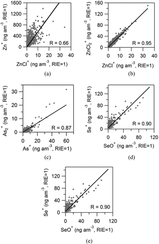
Comparison of estimated AMS ambient adduct-ion vs. elemental-ion signals of the same trace elements are shown in Figure 5. Input or difference signals were used depending on the ion, as explained previously. The scatter plots show a very good correlation (Pearson's R = 0.95) between the zinc chloride ions (ZnCl⁺ and ZnCl₂ ⁺, referred as ZnCl _x ⁺ hereafter), strongly suggesting that they were produced by the same compound in the ambient aerosol, most likely ZnCl₂. On the other hand, the correlation between Zn⁺ and ZnCl⁺ signals is lower (R = 0.66), which suggests that there was more than one zinc compound present in ambient particles: one more volatile, which also generates the ZnCl _x ⁺ ions; and another less volatile zinc compound, which might be Zn(NO₃)₂ (Moffet et al. 2008a). A similar finding was previously reported for Pb in this dataset, with PbCl⁺ ions being generated from fast evaporating species and other Pb ions being generated due to slowly evaporating species (Salcedo et al. 2010). Signals for As⁺ and As₂ ⁺ are highly correlated (R = 0.86), supporting the identification of both ions as arsenic and probably being generated by the same compound(s) in ambient particles. Correlation between all the Se-containing ions (Se⁺, SeO⁺, SeO₂ ⁺, etc.) is good, suggesting similar compounds/sources of the compounds generating the ions.

FIG. 5 Scatter plots of the adduct ion versus elemental ion signals of the same trace elements. Black lines are linear regression fits to the data with the intercept fixed at the origin. Pearson's R is shown.

3.3. Comparison to Other Instruments

The AMS-estimated elemental ambient concentrations are compared to the PIXE (PM_1.1) and ICP (PM_2.5) data in Figure 6. Cu, Sn, and Sb time series correspond to the ambient ion signals of Cu⁺, Sn⁺, and Sb⁺. Arsenic signal was calculated as the sum of the As⁺ and As₂ ⁺ ambient signals. For Zn and Se, a fraction of the ZnCl _x ⁺ and SeO _x ⁺ signals proportional to the mass fraction of the element was added to Zn⁺ and Se⁺ signals. No PIXE data for Sn and Sb, and no ICP data for Se were available. Figure 7 shows the scatter plots and regression lines comparing AMS with ICP and PIXE data. For these comparisons, averages of 6 and 12 h over the same time periods covered by the other instruments were performed on the AMS data. Linear regressions were performed using an Orthogonal Distance Regression (ODR) method, in order to take into account that the errors in both dependent and independent variables may be considerable (WaveMetrics 2008). Similar percent errors were assumed for both variables during the regressions. Scatter plots of AMS vs. PIXE-PM_0.3 are also shown. Comparisons of AMS with PIXE-PM_1.1 were always better than with PIXE-PM_0.3. The correlations between AMS and ICP were poor for Sn and Sb (Table 3, scatter plots not shown). Linear regressions were also performed on PIXE-PM_2.5 vs. ICP data, and the results are shown in Figure S21. In general, Person's R-values were relatively low for Cu, Zn, and As for PIXE vs. ICP. One possible cause of this discrepancy is the difference in sample volume and sampling time. Samples for ICP were collected using a high volume sampler (30 m³/h) for 12 h integrated samples (Querol et al. 2008), probing microgram to milligram of PM for each data point. In contrast, PIXE analysis probes only nanogram level of deposited material for each data point. The degree of correlation and agreement between the AMS and the other two methods is on the same range as that of the other two methods with each other.

TABLE 3 Reported cross-sections for single ionization by 70 eV electrons (Freund et al. 1990) and estimated relative ionization efficiencies (RIE _x ) from cross-sections

			AMS vs. PIXE1.1		AMS vs. ICP
	Cross	cross section
	section (Å)	RIE x from EI	R	Slope	R	Slope
Cu	3.47	0.61	0.41	0.27	0.27	0.06
Zn	–	–	0.72	0.75	0.55	0.93
As	5.69	0.88	0.56	0.48	0.15	0.77
Se	5.73	0.86	0.70	0.84	–	–
Sn	8.42	0.86	–	–	0.19	0.12
Sb	7.40	0.74	–	–	0.27	0.39
Note. Slope and Pearson's R from linear regression fits, using an Orthogonal Distance Regression (ODR) method with the intercept fixed at the origin, of AMS versus PIXE-PM1.1 and ICP data are also listed. The slope could be interpreted as RIE x , assuming that other causes of discrepancy are negligible.

In order to use the AMS as a quantitative tool to determine trace element concentrations, it is necessary to determine the RIE _x for each element, which can be estimated from the ratio of the absolute cross sections for electron single ionization at 70 eV and the number of electrons for the compound of interest and nitric acid (Jimenez et al. 2003). RIE _x estimated in this way for the trace elements detected with the AMS are shown in Table 3. In addition, the slopes of the correlation lines between AMS data (using RIE _x = 1) and PIXE or ICP data can be interpreted as the real RIE _x , assuming that the AMS sampled the same particles analyzed by the other instruments, and that the other technique's data were then used for calibration of the AMS. The slopes of the regression lines are listed in Table 3, along with the corresponding Pearson's R.

Table 3 shows that, in all cases, correlations for AMS are better when compared with PIXE than with ICP, which given the larger size cutoff for ICP, might be an indication that the trace elements are mainly contained in the supermicrometer fraction. There is a good correlation between AMS and PIXE-PM_1.1 data for Se, as well as a relatively good agreement between the two estimated RIE _x values; specially taking into account that both values are approximations to the true RIE _x . On the other hand, in the case of Cu, there is a poor correlation between AMS and PIXE-PM_1.1 or ICP data. RIE _x calculated from this comparison has a very small value (specially from ICP data), indicating that the other instruments report more Cu mass in the particles than the AMS. This is likely due to a significant fraction of the Cu being contained in particles larger than the AMS transmission window, and indeed the regression line has a slope much closer to 1 when using the PIXE PM_0.3 data (Figure 7). Another possible reason for part of the discrepancy is the presence of two types of Cu compounds, a less refractory one that the AMS detects and a very refractory one that the AMS cannot detect. Another possible reason for a low RIE _x is the fact that only the singly charged ions were used for the detection of copper (doubly charged ions were not detected above the noise level). However, if doubly charged ions could also be used, they would probably account for only a part of the discrepancy. A low correlation between PIXE-PM_2.5 and ICP (Figure S21) suggests that there might be other issues involved in Cu quantification, for example matrix effects or effects that depend on the chemical form of the element. For Sn and Sb, there is only ICP data to compare AMS data with, which show a poor correlation and very low estimated RIE _x from these comparisons (especially for Sn), suggesting that Sn and Sb might mainly be contained in the supermicrometer fraction.

FIG. 6 Comparison of estimated AMS ambient concentrations of trace elements, with PIXE and ICP measurements. Gray arrows indicate a peak off scale; numbers next to the arrows correspond to the maximum concentration of the peaks. (Color figure available online.)

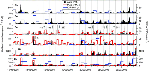
FIG. 7 Scatter plots of estimated AMS ambient concentrations of trace elements versus PIXE and ICP measurements. The results of linear regressions, using an ODR method with the intercept fixed at the origin, (lines, slopes [m] and Pearson's R) are shown. ICP data are not available for Se. Scatter plots for Sn and Sb are not shown because PIXE data are not available and correlations between AMS and ICP were very poor (Table 3).

However, because no PIXE data is available, it is not possible to compare with PM_0.3 data in order to determine if other issues are involved, as in the case of Cu. Although As presents poor correlations with ICP and PIXE-PM_1.1, the estimated RIE _x values from these comparisons are in good agreement with RIE _x from ionization cross-section. Finally, Zn presents a good correlation with PIXE-PM_1.1 and the estimated RIE _x is in the expected order of magnitude. Unfortunately, there is no cross-section data in the literature to compare to. Correlations between PIXE-PM_2.5 and ICP data for Cu, Zn, and As are very poor, suggesting that difficulties in the detection of these elements compounds are not exclusive of the AMS.

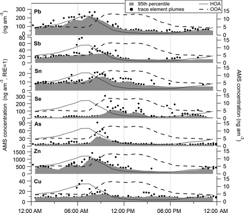
FIG. 8 Average diurnal cycles of the estimated AMS ambient concentrations of trace elements (black dots). Gray areas represent the 95th percentile of the data. Pb data from Salcedo et al. (2010) HOA and OOA PMF factors (Aiken et al. 2009) are also included.

It is important to note that the two methods to estimate RIE _x , discussed previously, are only approximations. Hence, the previous discussion intends to explore the potential of the AMS to be used quantitatively for the detection of trace elements in the airborne particles. It would be useful to determine RIE _x through laboratory experiments under controlled conditions, and using calibration materials in order to generate known concentrations of particles with known chemical composition. Furthermore, discrepancies were found when comparing AMS with ICP and PIXE measurements; however, comparison between these two instruments also showed disagreements and substantial scatter. Hence, laboratory experiments would also help to understand the differences seen between measurements using the three instruments.

3.4. Variability of Airborne Trace Elements

In order to explore variability of trace elements in the atmospheric aerosol of Mexico City, Figure 8 shows the diurnal cycle of the ambient concentrations of the elements discussed in this work vs. time of day.

FIG. 9 Comparisons of time series of the ambient AMS concentration for some trace element with other PM components during six time periods. Pb time series are from Salcedo et al. (2010). BBOA and LOA (PMF factors corresponding to biomass burning organic and a local primary nitrogen-containing organic aerosol, respectively) and chloride are from Aiken et al. (2009). (Color figure available online.)

The figure also shows the 95th percentile of the diurnal cycle of each trace element, to highlight the data points with the largest concentrations. Pb data from Salcedo et al. (2010) is also included, as well as the diurnal cycles of two aerosol organic fractions calculated by Aiken et al. (2009) using positive matrix factorization analysis (PMF, Ulbrich et al. 2009) on the same HR-AMS spectra discussed in here. The two PMF components shown in Figure 8 correspond to primary urban emissions (hydrocarbon-like organic aerosol, HOA) and to oxygenated organic aerosol (OOA) ascribed to photochemically formed secondary organic aerosol (SOA). In addition, the time series of the trace elements are plotted and compared with other particle components in Figure 9 for six selected time periods and for all the campaign in Figure 10. Sulfate, chloride, and BBOA and LOA (which correspond to two other PMF components corresponding to biomass organic and a local primary nitrogen-containing OA, respectively) were taken from Aiken et al. (2009). The three figures show that the highest concentrations of particle trace elements during the MILAGRO campaign occurred mainly during the morning hours; with the exception of Se, which showed maximum concentrations in the early afternoon. This is consistent with observations by Moreno et al. (2008), who noted a nightly increase in metal PM. However, their diurnal cycles are not similar to the HOA diurnal cycle; that is, largest concentrations of particle trace elements did not occur between 6 and 7 AM as HOA maximum concentrations did. In general, Cu, Se, and As, showed sharp plumes with large concentrations, and very low concentrations in between, indicating mainly local point sources (probably industrial) for these elements with small contributions for omnipresent area sources such as road traffic. Also, most trace elements had low concentrations during the holiday period in the middle of the campaign.

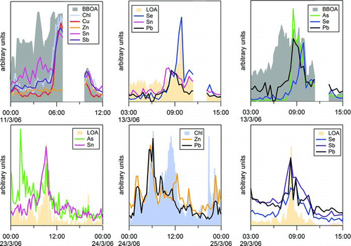
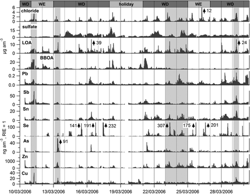
FIG. 10 Time series of the estimated AMS ambient concentration of trace elements. Pb time series are from Salcedo et al. (2010). BBOA and LOA (PMF factors corresponding to biomass burning organic and a local primary nitrogen-containing organic aerosol, respectively), sulfate, and chloride are from Aiken et al. (2009). The bar on top of the figure indicates weekends (WE), weekdays (WD), and holidays occurring during the campaign. Gray shadows indicate the time periods shown in Figure 9.

Industrial processing of copper is the largest source of Cu in the U.S.; however, urban dust is enriched with Cu, probably due to corrosion of automotive parts (Reff et al. 2009). Industrial sources may explain the sharp plumes, while the detected low-level background of Cu may represent some Cu enrichment in the submicron urban dust or other low-level sources. The main source of Se in the U.S. is coal combustion, which, however, is minor in the MCMA; hence, Se plumes may be of industrial origin. Most of man-made emissions of arsenic have their origin in metal smelters and the combustion of fuels; although, it might have a crustal origin as well (EC 2001). The former sources seem to be the most probable ones, causing the morning plumes observed. On the other hand, Zn, Sn, and Sb presented detectable background concentrations all the time, in addition to peaks during the morning. It is probable that these elements have area sources such as road traffic, as well as point sources causing the sharp plumes observed. For instance, Zn can be emitted by tire and brake wear; however, diesel engines also emit large quantities of Zn due to its use in antioxidants and as detergent/dispersant improvers in lubricating oils (Fergusson and Kim 1991; Smolders and Degryse 2002; Reff et al. 2009). Corrosion of galvanized-metal structures also contributes to large amounts of Zn in street dust (Fergusson and Kim 1991; Smolders and Degryse 2002), which is however less likely to be present in the submicron mode. Similarly, antimony had been thought to be emitted mainly by coal combustion and metallurgical processes. However, the use of Sb as flame retardant for plastics and chemical fabrics and lubricants for automotive brake friction materials, have increased the number of possible sources (Iijima et al. 2009). In fact, submicron antimony has been recently suggested as a tracer for trash burning in Mexico City (Christian et al. 2010; Hodzic et al. 2012).

Figure 9 shows that the composition of the plumes observed during the campaign varied widely; that is, the combination of trace elements and other particle components is different in each plume. The trace element plumes coincide sometimes with plumes of chloride, LOA, and/or BBOA, and most of such plumes contain only one or two trace elements.

All the above observations suggest that the sources of trace elements in Mexico City are very diverse in space and time, which is consistent with previous studies during the MCMA 2003 (Molina et al. 2007) and MILAGRO campaigns (Molina et al. 2010) that pointed toward mainly unidentified industrial sources for many trace elements (Johnson et al. 2006; Moffet et al. 2008a; Moreno et al. 2008; Adachi and Buseck 2010).

4. CONCLUSIONS

The detection and monitoring of trace elements in airborne particles is becoming an important research area as the anthropogenic sources of such elements increase in variety, size, and distribution, and toxicological studies find more evidence of potential health risks to humans. The HR-AMS has been widely used to study the chemical composition of the nonrefractory species that typically dominate submicron particles. In this work, we showed that the instrument (operated in the standard mode for nonrefractory species detection) is capable of detecting some important trace elements such as Cu, Zn, As, Se, Sn, and Sb, with high time resolution. The trace elements detected tend to be those of low melting/boiling points, consistent with the relatively low vaporizer temperature used in the AMS (600°C). Operation at vaporizer temperatures higher than 600°C might improve the detection of the semirefractory trace elements.

AMS spectral analysis, isotopic ratios, and ratios of different ions containing the same elements are used to confirm the chemical identity of the measured ions. Comparison of the AMS data with ICP and PIXE measurements was carried out in order to evaluate the potential and the difficulties involved in using the AMS as a quantitative tool for the detection of trace elements. Discrepancies were found between the three methods, which are likely related to inherent limitations in each of the analytical approaches, and can be additionally complicated by size distribution, sample size, and the chemical forms of each element involved. Hence, laboratory experiments under controlled conditions are necessary to understand these differences and the evaporation and detection of different chemical forms of the trace elements in the AMS.

Time series and diurnal cycles of the elements detected show sharp plumes in the morning hours. Zn, Sn, and Sb, also show detectable background levels most of the time. Associations of the trace elements with other particle components, such as biomass organic, nitrogen containing organic compounds, and chloride were found; however, such associations were very variable. All the observations suggest point sources, probably industrial, which are variable in time and space, which is in agreement with the previous findings in Mexico City.

Acknowledgments

This work was supported by the U.S. Department of Energy (DOE), Atmospheric System Research Program of the Office of Biological and Environmental Research (OBER) (contracts DE-SC0006035, DE-FG02–11ER65293, and DE-SC0001673), and Comisión Ambiental Metropolitana (México). The PIXE analysis was performed in the Environmental Molecular Sciences Laboratory, a national scientific user facility sponsored by OBER/DOE, and located at the Pacific Northwest National Laboratory (PNNL). PNNL is operated by the US DOE by Battelle Memorial Institute under contract DE-AC06–76RL0. We thank Xavier Querol at Instituto de Diagnostico Ambiental y Estudios del Agua, Spain, for providing the ICP MILAGRO data.

[Supplementary materials are available for this article. Go to the publisher's online edition of Aerosol Science and Technology to view the free supplementary files.]

REFERENCES

- Adachi , K. and Buseck , P. R. 2010 . Hosted and Free-Floating Metal-Bearing Atmospheric Nanoparticles in Mexico City . Environ. Sci. Technol. , 44 : 2299 – 2304 .
- Aiken , A. C. , DeCarlo , P. F. , Kroll , J. H. , Worsnop , D. R. , Huffman , J. A. Docherty , K. 2008 . O/C and OM/OC Ratios of Primary, Secondary, and Ambient Organic Aerosols with High Resolution Time-of-Flight Aerosol Mass Spectrometry . Environ. Sci. Technol. , 42 : 4478 – 4485 .
- Aiken , A. C. , deFoy , B. , Wiedinmyer , C. , DeCarlo , P. F. , Ulbrich , I. M. Wehrli , M. N. 2010 . Mexico City Aerosol Analysis during MILAGRO using High Resolution Aerosol Mass Spectrometry at the Urban Supersite (T0). Part 2: Analysis of the Biomass Burning Contribution and the Modern Carbon Fraction . Atmos. Chem. Phys. , 10 : 5315 – 5341 .
- Aiken , A. C. , Salcedo , D. , Cubison , M. J. , Huffman , J. A. , DeCarlo , P. F. Ulbrich , I. M. 2009 . Analysis during MILAGRO using High Resolution Aerosol Mass Spectrometry at the Urban Supersite (T0). Part 1: Overall Fine Particle Composition and Organic Source Apportionment . Atmos. Chem. Phys. , 9 : 6633 – 6653 .
- Allan , J. D. , Alfarra , M. R. , Bower , K. N. , Williams , P. I. , Gallagher , M. W. Jimenez , J. L. 2003 . Quantitative Sampling Using an Aerodyne Aerosol Mass Spectrometer 2. Measurements of Fine Particulate Chemical Composition in two U.K. Cities . J. Geophys. Res. , 108 : 4099 – 4105 .
- Baron , P. A. and Willeke , K. 2001 . Aerosol Measurements. Principles, Techniques, and Applications , New York , , USA : John Wiley & Sons .
- Canagaratna , M. R. , Jayne , J. T. , Jimenez , J. L. , Allan , J. D. , Alfarra , M. R. Zhang , Q. 2007 . Chemical and Microphysical Characterization of Ambient Aerosols with the Aerodyne Aerosol Mass Spectrometer . Mass Spectrom. Rev. , 26 : 185 – 222 .
- Charlesworth , S. , DeMiguel , E. and Ordóñez , A. 2011 . A Review of the Distribution of Particulate Trace Elements in Urban Terrestrial Environments and its Application to Considerations of Risk . Environ. Geochem. Health , 33 : 103 – 123 .
- Christian , T. J. , Yokelson , R. J. , Cárdenas , B. , Molina , L. T. , Engling , G. and Hsu , S. C. 2010 . Trace Gas and Particle Emissions from Domestic and Industrial Biofuel Use and Garbage Burning in Central Mexico . Atmos. Chem. Phys. , 10 : 565 – 584 .
- DeCarlo , P. F. , Kimmel , J. R. , Trimborn , A. , Northway , M. J. , Jayne , J. T. Aiken , A. C. 2006 . Field-Deployable, High-Resolution, Time-of-Flight Aerosol Mass Spectrometer . Anal. Chem. , 78 : 8281 – 8289 .
- deLaeter , J. R. , Böhlke , J. K. , deBièvre , P. , Hidaka , H. , Peiser , H. S. Rosman , K. J. R. 2003 . Atomic Weights of the Elements: Review 2000 (IUPAC Technical Report) . Pure Appl. Chem. , 75 : 683 – 800 .
- Drewnick , F. , Hings , S. S. , Curtius , J. , Eerdekens , G. and Williams , J. 2006 . Measurement of Fine Particulate and Gas-phase Species During the New Year's Fireworks 2005 in Mainz, Germany . Atmos. Environ. , 40 : 4316 – 4327 .
- EC . 2001 . Ambient Air Pollution by As, Cd and Ni Compounds Position Paper, European Comission. EG environment, Luxembourg
- EP . 2008 . Directive 2008/50/EC of the European Parliament and of the Council of 21 May 2008 on Ambient Air Quality and Cleaner Air for Europe, Official Journal of the European Union, L52, Luxembourg .
- EPA . 1999 . Particulate Matter (PM2.5) Speciation Guidance, 1st ed., Final Draft, U.S. Environmental Protection Agency, Research Triangle Park, NC, USA .
- Fergusson , J. E. and Kim , N. D. 1991 . Trace Elements in Street and House Dusts: Sources and Speciation . Sci. Total Environ. , 100 : 125 – 150 .
- Franklin , M. , Koutrakis , P. and Schwartz , J. 2008 . The Role of Particle Composition on the Association between PM2.5 and Mortality . Epidemiology , 19 : 680 – 689 .
- Freund , R. S. , Wetzel , R. C. , Shul , R. J. and Hayes , T. R. 1990 . Cross-Section Measurements for Electron-Impact Ionization of Atoms . Phys. Rev. A , 41 : 3575 – 3595 .
- Hodzic , A. , Wiedinmyer , C. , Salcedo , D. and Jimenez , J. L. 2012 . Impact of Trash Burning on Air Quality in Mexico City . Environ. Sci. Technol. , 46 : 4950 – 4957 .
- Huffman , J. A. , Docherty , K. S. , Mohr , C. , Cubison , M. J. , Ulbrich , I. M. Ziemann , P. J. 2009 . Chemically-Resolved Volatility Measurements of Organic Aerosol from Different Sources . Environ. Sci. Technol. , 43 : 5351 – 5357 .
- Iijima , A. , Sato , K. , Fujitani , Y. , Fujimori , E. , Saito , Y. Tanabe , K. 2009 . Clarification of the Predominant Emission Sources of Antimony in Airborne Particulate Matter and Estimation of their Effects on the Atmosphere in Japan . Environ. Chem. , 6 : 122 – 132 .
- Järup , L. 2003 . Hazards of Heavy Metal Contamination . Br. Med. Bull. , 68 : 167 – 182 .
- Jimenez , J. L. , Jayne , J. T. , Shi , Q. , Kolb , C. E. , Worsnop , D. R. Yourshaw , I. 2003 . Ambient Aerosol Sampling Using the Aerodyne Aerosol Mass Spectrometer . J. Geophys. Res. , 108 : 8425
- Johnson , K. S. , Foy , B. d. , Zuberi , B. , Molina , L. T. , Molina , M. J. Xie , Y. 2006 . Aerosol Composition and Source Apportionment in the Mexico City Metropolitan Area with PIXE/PESA/STIM and Multivariate Analysis . Atmos. Chem. Phys. , 6 : 4591 – 4600 .
- Kleinman , L. I. , Springston , S. R. , Daum , P. H. , Lee , Y. N. , Nunnermacker , L. J. Senum , G. I. 2008 . The Time Evolution of Aerosol Composition Over the Mexico City Plateau . Atmos. Chem. Phys. , 8 : 1559 – 1575 .
- Lee , T. , Sullivan , A. P. , Mack , L. , Jimenez , J. L. , Kreidenweis , S. M. Onasch , T. B. 2010 . Variation of Chemical Smoke Marker Emissions During Flaming vs. Smoldering Phases of Laboratory Open Burning of Wildland Fuels . Aerosol Sci. Technol. , 44 : i – v .
- Lide , D. R. 2008 . CRC Handbook of Chemistry and Physics , Boca Raton : CRC Press .
- Lippmann , M. 2009 . Semi-Continous Speciation Analyses for Ambient Air Particulate Matter: An Urgent Need for Health Effects Studies . J. Exposure Sci. Environ. Epidemiol. , 19 : 235 – 247 .
- Middlebrook , A. M. , Bahreini , R. , Jimenez , J. L. and Canagaratna , M. R. 2012 . Evaluation of Composition-Dependent Collection Efficiencies for the Aerodyne Aerosol Mass Spectrometer using Field Data . Aerosol Sci. Technol. , 46 : 258 – 271 .
- Moffet , R. C. , Desyaterik , Y. , Hopkins , R. J. , Tavanski , A. V. , Gilles , M. K. Wang , Y. 2008a . Characterization of Aerosols Containing Zn, Pb, and Cl from an, Industrial Region of Mexico City . Environ. Sci. Technol. , 42 : 7091 – 7097 .
- Moffet , R. C. , Foy , B. d. , Molina , L. T. , Molina , M. J. and Prather , A. 2008b . Measurement of Ambient Aerosols in Northern Mexico City by Single Particle Mass Spectrometry . Atmos. Chem. Phys. , 8 : 4499 – 4516 .
- Moffet , R. C. , Henn , T. R. , Tivanski , A. V. , Hopkins , R. J. , Desyaterik , Y. Kilcoyne , A. L. D. 2010 . Microscopic Characterization of Carbonaceous Aerosol Particle Aging in the Outflow from Mexico City . Atmos. Chem. Phys. , 10 : 961 – 976 .
- Molina , L. T. , Kolb , C. E. , de Foy , B. , Lamb , B. K. , Brune , W. H. Jimenez , J. L. 2007 . Air Quality in North America's Most Populous City—Overview of the MCMA-2003 Campaign . Atmos. Chem. Phys. , 7 : 2447 – 2473 .
- Molina , L. T. , Madronich , S. , Gaffney , J. S. , Apel , E. , deFoy , B. Fast , J. 2010 . An Overview of MILAGRO 2006 Campaign: Mexico City Emissions and their Transport and Transformation . Atmos. Chem. Phys. , 10 : 8697 – 8760 .
- Moreno , T. , Querol , X. , Pey , J. , Minguillón , M. C. , Pérez , N. Alastuey , A. 2008 . Spatial and Temporal Variations in Inhalable CuZnPb Aerosols within the Mexico City Pollution Plume . J. Environ. Monit. , 10 : 370 – 378 .
- Mugica , V. , Ortiz , E. , Molina , L. , Vizcaya-Ruiz , A. D. , Nebot , A. Quintana , R. 2009 . PM Composition and Source Reconciliation in Mexico City . Atmos. Environ. , 43 : 5068 – 5074 .
- Pope , C. A. and Dockery , D. W. 2006 . Health Effects of Fine Particulate Air Pollution: Lines that Connect . J. Air Waste Manage. Assoc. , 56 : 709 – 742 .
- Querol , X. , Pey , J. , Minguillón , M. C. , Pérez , N. , Alastuey , A. Viana , M. 2008 . PM Speciation and Sources in Mexico During the MILAGRO-2006 Campaign . Atmos. Chem. Phys. , 8 : 111 – 128 .
- Reff , A. , Bhave , P. V. , Simon , H. , Pace , T. G. , Pouliot , G. A. Mobley , J. D. 2009 . Emissions Inventory of PM2.5 Trace Elements across the United States . Environ. Sci. Technol. , 43 : 5790 – 5796 .
- Richard , A. , Bukowiecki , N. , Lienemann , P. , Furger , M. , Fierz , M. Minguillon , M. C. 2010 . Quantitative Sampling and Analysis of Trace Elements in Atmospheric Aerosols: Impactor Characterization and Synchrotron-XRF Mass Calibration . Atmos. Meas. Tech. , 3 : 1473 – 1485 .
- Salcedo , D. , Onasch , T. B. , Aiken , A. C. , Williams , L. R. , de Foy , B. Cubison , M. J. 2010 . Determination of Particulate Lead Using Aerosol Mass Spectrometry: MILAGRO/MCMA-2006 Observations . Atmos. Chem. Phys. , 10 : 5371 – 5389 .
- Salcedo , D. , Onasch , T. B. , Dzepina , K. , Canagaratna , M. R. , Zhang , Q. Huffman , J. A. 2006 . Characterization of Ambient Aerosols in Mexico City During the MCMA-2003 Campaign with Aerosol Mass Spectrometry: Results from the CENICA Supersite . Atmos. Chem. Phys. , 6 : 925 – 946 .
- Shutthanandan , V. , Thevuthasan , S. , Disselkamp , R. , Stroud , A. , Cavanagh , A. Adams , E. M. 2002 . Development of PIXE, PESA and Transmission Ion Microscopy Capability to Measure Aerosols by Size and Time . Nucl. Instrum. Methods Phys. Res.: Sect. B , 189 : 284 – 288 .
- Smolders , E. and Degryse , F. 2002 . Fate and Effect of Zinc from Tire Debris in Soil . Environ. Sci. Technol. , 36 : 3706 – 3710 .
- Ulbrich , I. M. , Canagaratna , M. R. , Zhang , Q. , Worsnop , D. R. and Jimenez , J. L. 2009 . Interpretation of Organic Components from Positive Matrix Factorization of Aerosol Mass Spectrometric Data . Atmos. Chem. Phys. , 9 : 2891 – 2918 .
- WaveMetrics . 2008 . IGOR Pro. V6.0. User's Guide , Portland , , OR, USA : WaveMetrics, Inc. .
- Wong , C. S. C. , Li , X. and Thornton , I. 2006 . Urban Environmental Geochemistry of Trace Metals . Environ. Pollut. , 142 : 1 – 16 .