Population Balances of Micron-Sized Aerosols in a Bipolar Ion Environment

Abstract

The present work re-examines the assumptions that are required for a steady-state charge distribution analysis to be valid. First, the common approximation that there are only 11 charge states available to the distribution is relaxed to allow for 201 charge states to be available to the particle distribution. This is found to have large repercussions on the behavior of the distribution for radii greater than 0.5 μm. The steady-state assumption itself is then re-examined by calculating the time required to reach steady state for many different ion-pair production rates and initial particle charge states as a function of radius. In the steady-state model, the ion populations are often assumed to decouple completely from the aerosol; this is shown to be false throughout the troposphere. Finally, the number of positive and negative charge states needed to accurately model a particle population of a given size is determined.

© 2013 American Association for Aerosol Research

INTRODUCTION

The greatest source of uncertainty in aerosol mobility analysis is the fraction of particles that is counted, largely due to the small number of particles that are charged. Size distribution measurements made using the differential mobility analyzer, DMA, to classify particles according to size therefore require accurate knowledge of the aerosol charge distribution as a function of particle radius (Hoppel and Frick 1986; Biskos 2004). Quantitative analysis of aerosols is of paramount importance in understanding the chemical and physical processes that govern atmospheric particle formation and growth. In ambient measurements, errors in the charge distribution could cause nucleation events to be mistaken as noise. To measure aerosol yields in chamber studies, the particle size distribution is monitored as particles grow. Biases due to imperfect knowledge of the fraction of particles that carry charge and that can, therefore, be classified may introduce substantial error in estimates of the amount of secondary organic aerosol formed, a key parameter in studies of the role of aerosols in climate change.

Charge transfer is a well-studied kinetic process, yet questions remain. In the transition size regime, the classic studies by Natanson (1960), Fuchs (1963), and Keefe et al. (1968) describe an ion current through a “limiting sphere.” Inside the sphere, one is in the free molecular regime; outside the sphere, one is in the continuum regime. At the boundary, the currents must be equal. Work has continued on the problem since then with contributions from studies by Hoppel and Frick (1986) and Lushnikov and Kulmala (2004a,b), among others. In the present article, we examine the charge distribution over particles between 1 nm and 10 m, using the Hoppel and Frick (1986) model, henceforth referred to as HF, which extended the classical description and numerically evaluated the steady-state charge distribution for bipolar, diffusive charging. As in HF, we focus here on the steady-state charge distribution while relaxing computational limitations that were imposed in that earlier work. This steady-state charge distribution both describes the charge state of the atmospheric aerosol and provides the fraction in each possible charge state that is needed to deduce the particle size distribution from mobility analysis data. The present analysis shows that computational limitations in the range of charge states and average ion speeds considered by HF profoundly affect the charge distribution at the upper end of the mobility analysis size range. The resulting changes in the estimated fraction of charged particles are important in estimations of the aerosol mass and volume from DMA measurements.

MODELS

To deduce the statistical macroscopic charge state of a monodisperse aerosol from the attachment coefficient, one must solve a system of balance equations that describe the time evolution of the ion and aerosol populations (Isreal 1971). These are simply coupled rate equations, just as are found in model chemical reactions. Assuming a single ion species for each polarity, the ion concentrations, n ₁ and n ₋₁, are described by

and

where N_k is the concentration of particles with charge state k, and q is the rate of creation of new ions per unit volume. Ion recombination is proportional to the product of the concentrations of positive and negative ions; α is the so-called recombination rate coefficient. In the limit of low particle concentrations, N, n ₁ and n ₋₁ are determined by ion recombination, and the loss of ions to aerosol particles can be decoupled from the ion kinetics. More generally, the particles can influence the ion population, as indicated by the summation of ion-particle charge scavenging rates over the particle charge state k.

The ion attachment coefficients, β _k,i , determine the charge distribution, and are calculated as described by the HF model with one exception. The HF model uses two average “characteristic” ion kinetic energies to describe the ion–particle interaction: 4k _B T/π for uncharged particles and k _B T for charged particles, where k _B is the Boltzmann constant and T is temperature. This is a subset of the five “characteristic” kinetic energies described by Keefe et al. (1968). Four energies will be used here: 4k _B T/π for uncharged particles, k _B T for attractive interactions with charged particles, 1.25k _B T for attractive interactions with charged particles larger than 1 m, and 1.5k _B T for repulsive interactions. This slight extension will improve the estimate of the required number of charge states as a function of particle size later in this article.

The ions are assumed to carry only one elementary charge, a good approximation in the limit of small ions. The time evolution of the aerosol population is

assuming that there are no particle sources or sinks and that the particles only change charge states through ion attachment. It then logically follows that the total charge per unit volume,

and total particle concentration,

are conserved. Equations (1)–(5) can be solved to determine the time-dependent charge distribution.

In bipolar diffusion charging, the charge distribution asymptotically approaches a steady state at which

The ratio of concentrations in successive charge states is found to be

For k→K large enough such that both and are arbitrarily close to 0, Equation (6) can be approximated ¹ by

The steady-state approximation implies that Equation (7) is true for all k. In the past, this relationship has been incorrectly invoked without proof as an expression of microscopic reversibility, which would imply that a captured charge can be re-emitted by the capturing particle. The rate of such charge emission is negligible near room temperature, so charge equilibrium will not be established on any reasonable time scale. Instead, charged particle neutralization occurs via preferential attachment of ions with charge opposite of that of the particle, leading to the hypothesized steady-state charge distribution.

We may relate the concentration of particles in a given charge state to that of neutral particles by multiplying successive concentration ratios, i.e.,

This number can be used to construct the ratio of the total particle concentration to that of neutral particles,

where K ⁺ is the maximum charge state k considered in the positive direction and K ⁻ is the maximum charge state k considered in the negative direction. The fraction of particles in charge state k then becomes

Similar expressions can be obtained for negatively charged particles. It is worth noting that the value for K ⁺ or K ⁻ that is needed to account for all charged particles is strongly size dependent, e.g., virtually no particles smaller than 10 nm will acquire more than one charge, while most supermicron particles will be multiply charged. The limiting k values in the positive and negative directions are not necessarily symmetric due to differences in the mobilities of positive and negative ions. In plasma environments, which rely on the same underlying physics, particles can actually hold a large fraction of the negative charge in the system (Khrapac and Morfill 2009). In this study, the values for mobility and mass from HF of: 150 AMU and 1.2·10⁻⁴ m²/(V·s) for positive ions and 90 AMU and 1.35·10⁻⁴ m²/(V·s) for negative ions are used.

In the discussion that follows, we examine the effect of the values of K ⁺ and K ⁻ on the estimate of the steady-state charge distribution, extending our calculations well beyond the limits employed by HF, K ⁺ _HF=K ⁻ _HF=5; this value was chosen to model particles of up to ∼500 nm in radius at typical atmospheric conditions. One reason for this cutoff was computational limitations of the time. In our return to this topic, we first examine the steady-state charge distribution and the number of charges, K ^±, that must be considered. We then explore the time required to achieve that steady-state distribution, and the effect of the ion production rate on both the charge distribution and the time required to achieve it by using a transient model, which was integrated using a fifth-order Runge–Kutta–Fehlberg algorithm. The transient model assumes that creation and destruction of ions occur uniformly throughout the volume and that the equations describing the evolution of the population of ions and the aerosol are not decoupled, as they were in the HF model.

RESULTS AND DISCUSSION

In the following discussion, we consider the addition of more “characteristic” kinetic energies in the calculation of flux coefficients and the determination of flux coefficients for high charge states that were excluded from the calculations of HF. The flux coefficients calculated using the HF model and the present model are shown in Figure 1. The inclusion of more kinetic energies leads to a slight enhancement in the flux coefficient during repulsive interactions for particles less than 200 nm in radius. Otherwise the present model agrees well with the HF model for all flux coefficients previously calculated. Although the effect of this extension to HF on the flux coefficients is small, it will eliminate nonphysical behavior as we evaluate the effects of truncating the sums in calculating the steady-state charge distribution.

FIG. 1 Flux coefficients for (a) negative and (b) positive ions to aerosol particles of various charge states. (Color figure available online.)

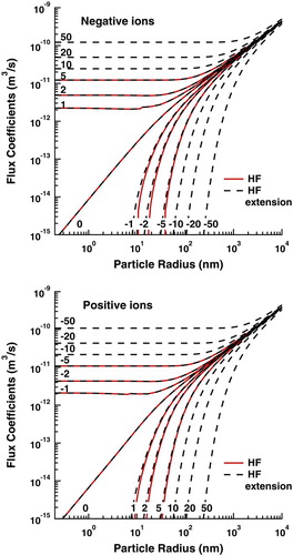
FIG. 2 The product of the ion concentration and the time to reach steady state as a function of particle radius. Each curve represents a different starting charge for the particle population. (Color figure available online.)

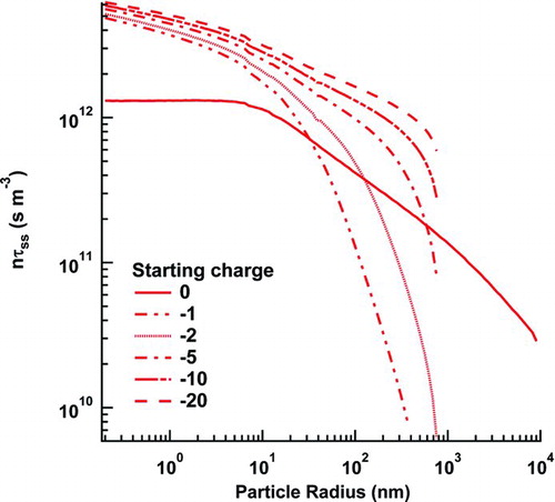
Before we discuss the resultant steady-state charge distribution from these flux coefficients, we should ask a much more basic question: Is the steady-state approximation valid for the DMA measurements to which they are normally applied? To answer this, we undertook a general study of nτ_ss, where τ_ss is the time it takes the charged fraction of the particle population to reach steady state, as a function of particle size, and n is the negative ion population (which varies by <10% from the positive ion population in all subsequent calculations). These transient simulations examine ion–aerosol systems in which the ion-pair creation rate was varied between 4.33·10¹¹ ions/(cm³·s), a typical ion-pair production rate for a 2 mCi Po neutralizer (Cooper and Reist 1973), and 2 ions/(cm³·s), the rate at the bottom of the troposphere. The recombination rate coefficient was held at 3·10⁻⁶ cm³/s (Cooper and Reist 1973), and the aerosol concentration was held at 10 particles/cm³, with all particles beginning neutral. For all of these cases, τ_ss was defined as the time it takes for the charged particle population to reach 90% of its asymptote. The results are shown in Figure 2 as a function of particle size. No significant changes were observed to result from changing the ion-pair production rates. However, a spot check at different initial particle charges led to significant changes in nτ_ss. This deviation suggests that the initial particle charge distribution may have a significant effect on τ_ss; τ_ss becomes undefined at large particle size for all the initially charged particle populations because the final charged particle population deviates no more than 10% from the initial charged particle population or because the value overshoots by greater than 10% after first approach. More concretely, for an aerosol population that begins neutral, the time to achieve 99% of the steady-state value was 6 ms or less for 1 nm to 10 m radii particles with concentrations ranging from 10 to 10⁶ particles/cm³ at ion concentrations of 3.8·10⁸ ions/cm³. At a concentration of 10⁷ particles/cm³ with particles of 10 m radius, the time increased to 17 ms at the same ion concentration. With typical residence times of 3 s or greater in a neutralizer, the aerosol particles achieve the steady-state charge distribution within the neutralizer.

FIG. 3 Steady-state charge distributions for (a) the HF model and (b) the HF extended model. (Color figure available online.)

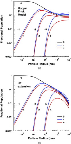
The resultant steady-state charge distributions calculated using K ⁺=K ⁻=5, as in the HF model, is shown in Figure 3. Here it is compared with the distribution calculated by extending the HF model to K ⁺=K ⁻=100 and including more “characteristic” kinetic energies. This more closely approximates the full Maxwellian ion velocity distribution. The truncation of the ion charge in the HF model leads all charge states to approach an asymptote at large particle sizes. In contrast, when the charge states are not so artificially bound, the fraction of particles in any given charge state decreases with size, but the fraction of charged particles (k≠0) asymptotically approaches unity. In contrast, the inclusion of the extra kinetic energies leads to only small shifts in the distribution, most readily noted in the populations of doubly charged aerosol at small size.

There is one other possible source of deviation that bears mentioning at this point. At high aerosol loading or low ion-pair production, the assumption made in the steady-state solutions that the aerosol and ion population evolution are decoupled breaks down at larger particle radii. Here, the population of highly charged states seriously alters the steady-state ion concentration. For 10 m particles, this results in a deviation of 0.6%, 6%, 76%, and 260% from the decoupled solutions for concentrations of 10⁴, 10⁵, 10⁶, and 10⁷ particles/cm³ respectively, assuming an ion-pair production rate of 4.33·10¹¹ ions/(cm³·s). This creates a distribution that lies somewhere between the original HF results and the present results. This population coupling is also exhibited in complex plasmas and in the troposphere due to the low ion-pair production rates there. Figure 4 shows the bottom, 2 ions/(cm³·s) and 10 particles/cm³, of the troposphere with low aerosol loading. Further enhancement of the aerosol population or decrease in ion-pair production will only exaggerate the distortion.

FIG. 4 At large particle size, the steady-state distribution in the troposphere is altered by the strong coupling between the ion and aerosol populations. This figure shows the distribution at the bottom of the atmosphere where the ion-pair production rate, ∼2 ions/(cm³·s), is at its lowest, leading to the largest distortion. (Color figure available online.)

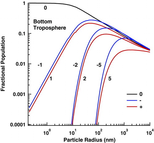
FIG. 5 The fraction of the aerosol in a neutral charge state is given as a function of maximum, negative charge, K ⁻, in (a), where the solid circles show the points at 99% of the asymptotic values. These latter points are given as a function of particle size and fitted in (b), while the inset graphs show the charge distribution at a given size. (Color figure available online.)

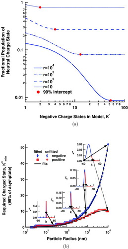
For the purpose of calculating both the transient and steady-state solutions described above, K ^± was assumed to be 100. However, this is far more terms than the calculation actually requires. A minimum value for each polarity must be established. To that end, Figure 5a  presents the relationship between the fraction of the aerosol in a neutral charge state and the maximum number of negative charge states, K ⁻, allowed in the model. From this, we can infer K ⁻ _min, the minimum number of negative charge states required to accurately describe the charge distribution at a given particle size. The points of charge K ⁻ _min are represented as solid circles in Figure 5a. They are defined as the point where the aerosol fraction reaches 99% of its asymptotic value. K ⁺ _min can be determined in a similar fashion. K ^± _min are plotted as a function of particle size in Figure 5b. The insets to this graph show discrete charge distributions at a few selected sizes. They show that the particle size and ion mobility greatly skew the resultant distribution.

Because charge is quantized, the increase in K ^± _min with respect to particle radius occurs in discrete steps. The points at the edge of each of these steps, represented in Figure 5b as a filled diamond or a square with a cross through it, are fit to find the underlying functional form. The much greater mobility of the negative ions is shown to cause a wide disparity in the minimum number of charge states required for each polarity and in their functional form. K ⁻ _min follows a power law,

where C ₀=(1.016 ± .041)·10⁵ m^−t , t=0.6597 ± 0.0033, and a is the particle radius. The additional ion kinetic energies mentioned above reduce the error in this fit. K ⁺ _min, instead, follows a log normal distribution,

where C ₁=10.55±0.19, a ₀=(8.25±1.25)·10⁻⁶ m, and w=3.42 ± 0.16 m. The underlying physical reason for this behavior is beyond the scope of this study, but the functional forms shown here may still allow others to budget their computing resources more appropriately.

CONCLUSIONS

The HF model has been extended to include higher charge states and more “characteristic” ion kinetic energies than in earlier HF analysis. This does little to affect the previously calculated flux coefficients, but the higher charge states prove very important at large particle radius, where it becomes increasingly likely that these states are populated. This creates huge differences in the resultant steady-state distribution at large size, where the previous model approaches an artificial asymptote at all charge states, but the current model has a decreasing fractional population at all charge states.

The assumption that the particle charge distribution reaches steady state for typical experimental neutralizer setups is also re-examined and found valid. A general dependence of the time required to achieve steady state as a function of particle size and initial particle charging is shown. The assumption that the ion and aerosol populations can be decoupled is verified for the most common cases. General calculations of the time to reach steady state based on the particle size and a few individual charge states are provided.

The assumption that the two populations under consideration, ions and particles, are decoupled is found to be dependent on aerosol loading and particle size; it is valid to within 6% for all particle sizes up to an aerosol concentration of 10⁵ particles/cm within a typical neutralizer. Calculating the minimum charge state necessary to accurately model a particle population of a given size allows us to determine a functional dependence with respect to the radius. We find that the negative charge states follow a power law, while the positive charge states follow a log normal distribution due to the large difference in their mobilities. Including more characteristic ion energies proves useful in reducing the error of this calculated power law. This raises several questions about the kinetics of ion capture and, specifically, the approximation of an average ion velocity. These concerns will be addressed in a article to follow.

Acknowledgments

We thank Andrew Downard for his time spent editing and discussing this manuscript. We would also like to thank the NASA Astrobiology Institute through the NAI Titan team managed at JPL under NASA Contract NAS7-03001 for the funding of this project, and the Ayrshire Foundation for their support in making computing resources available.

Notes

See the appendix for details.

APPENDIX: LIMIT OF CHARGE RATIO

The ratio of concentration in successive charge states was earlier found to be

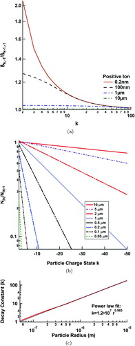
FIG. 6 Ratios of sequential positive ion flux coefficients, β _k /β _k−1, and sequential charged populations, N _|k|/N _|k|−1, versus charge state, k. The size dependence of the decay constant for N _|k|/N _|k|−1 is also shown. (Color figure available online.)

In order to evaluate the full steady-state charge distribution, it is instructive, at this point, to examine the asymptotic behavior of and as k→∞. The former ratio, shown in Figure A1a, approaches 1 at large k. This is to be expected since, for a large enough absolute value of k, a difference of 1 charge is fractionally insignificant to the potential. We see a strong size dependence, with the largest changes per charge step occurring in the kinetic regime, while the continuum regime shows little change throughout. This is potentially caused by increasing the collision cross-section between an ion and a particle within the limiting sphere, but only up to the size of the limiting sphere. In the continuum regime, where the particles are already very near the size of the limiting sphere, the captured cross-section is almost unaffected. The latter ratio, that of the charged populations, is calculated by running the transient model until steady-state values are achieved. The results, shown here in Figure A1b, follow an exponential decay, approaching 0 with increasing k across all particle sizes. The constant of this decay follows a power law relationship with respect to particle size as shown in Figure A1c and is very nearly linear above 300 nm. This physical behavior agrees with our intuition. Each successive charge state becomes harder to fill, and the population of successive charge states drops precipitously. Large particles can more easily support higher charge states because of the increased distance between charges.

Applying these results to Equation (A1), we can make simplifications. The third factor in the denominator on the right hand side of the expression,

has two additive terms that both independently approach 0. The second term in Equation (A2) becomes vanishingly small as forces between a highly charged particle and an ion increase. This leads to a vanishingly small flux for the repulsive case in the numerator and a large flux for the attractive case in the denominator. In the third term, the factor goes to 1. Figure A1b shows that for large k at all sizes. For k→K large enough such that both terms are arbitrarily close to 0, Equation (A1) can be approximated by

REFERENCES

- Biskos , G. 2004 . Theoretical and Experimental Investigation of the Differential Mobility Spectrometer , Cambridge : University of Cambridge .
- Cooper , D. W. and Reist , P. C. 1973 . Neutralizing Charged Aerosol with Radioactive Sources . J. Colloid Interface Sci. , 45 ( 1 ) : 17 – 26 .
- Fuchs , N. A. 1963 . On the Stationary Charge Distribution on Aerosol Particles in a Bipolar Ionic Environment . Geofis. Pura Appl. , 56 : 185 – 192 .
- Hoppel , W. A. and Frick , G. M. 1986 . Ion-Aerosol Attachment Coefficients and the Steady-State Charge Distribution on Aerosols in a Bipolar Ion Environment . Aerosol Sci. Technol. , 5 : 1 – 21 .
- Isreal , H. 1971 . Atmospheric Electricity , Jerusalem : Israel Program for Scientific Translations .
- Keefe , D. , Nolan , P. J. and Scott , J. A. 1968 . Influence of Coulomb and Image Forces in Combination of Aerosol . Proc. R. Irish. Acad. , 60A : 27 – 44 .
- Khrapac , S. and Morfill , G. 2009 . Basic Processes in Complex (Dusty) Plasmas: Charging, Interactions, and Ion Drag Force . Contrib. Plasma Phys. , 49 ( 3 ) : 148 – 168 .
- Lushnikov , A. A. and Kulmala , M. 2004a . Flux-Matching Theory of Particle Charging . Phys. Rev. E. , 70 : 046413
- Lushnikov , A. A. and Kulmala , M. 2004b . Charging of Aerosol Particles in the Near Free-Molecule Regime . Eur. Phys. J. D , 29 : 345 – 355 .
- Natanson , G. L. 1960 . On the Theory of Charging of Amicroscopic Aerosol Particles as a Result of the Capture of Gas Ions . Soviet Phy. Tech. Phys. , 5 : 538 – 551 .