The Suitability of Particle Models in Capturing Aggregate Structure and Polydispersity

Abstract

This work presents the mathematical formulation of particle models commonly used in aerosol dynamics of nanoparticles. A detailed numerical study is conducted in order to understand under which conditions these models differ. The silica model of Shekar et al. (2012b) and silicon model of Menz et al. (2013) taken from the literature are analyzed using three different particle models, demonstrating that substantial errors can be incurred when using a particle model inappropriate for a particular modeling application. These errors can potentially be reflected in fitted parameters; should a parameter estimation procedure be employed with such models. It is concluded that the characteristic coagulation and sintering timescales define the conditions under which the use of a particular model is reasonable.

Copyright 2013 American Association for Aerosol Research

1. INTRODUCTION

Population balance modeling is typically applied in order to model the aerosol synthesis of nanoparticles (Xiong and Pratsinis 1993; Tsantilis et al. 2002; Kraft 2005). Depending on how the population balance equations are solved, different assumptions are made about the nature of the particles to simplify these equations’ solutions (Xiong and Pratsinis 1993). The level of detail to which the particles are described is defined as a particle model.

The aerosol system to be modeled and the population balance equation solution methodology typically define which particle model is used. Three main categories of solution methodology are employed. The “method of moments” (Frenklach and Harris 1987; Frenklach 2002) describes the evolution of a population of particles by the moments of the distribution. It is typically fast; however, the particle size distribution (PSD) cannot be resolved from the results of such calculations. The sectional methods split the distribution of particle properties into sections (Hounslow 1990), allowing some resolution of PSD. These methods are often more computationally expensive (Xiong and Pratsinis 1993) than the moments method and can only be extended to multiple internal dimensions with great difficulty (Heine and Pratsinis 2007).

An alternative is to use stochastic methods (Balthasar and Kraft 2003; Patterson et al. 2006a,b, 2011; Celnik et al. 2007): these approximate the real particles with a collection of “computational particles.” The computational particles may interact with each other through a series of stochastic jump processes which define how the particles change with time. These methods have been applied to a variety of systems (Celnik et al. 2007; Sander et al. 2009, 2011; Shekar et al. 2012a; Chen et al. 2013; Menz and Kraft 2013). However, the main disadvantage of stochastic methods is that it is difficult to include spatial inhomogeneity (Patterson et al. 2011; Patterson and Wagner 2012).

In early modeling attempts, particles were treated as spheres which would coalesce into larger spheres upon collision with other particles; for example, see Frenklach and Harris (1987). This corresponds to the spherical particle model; which is a one-dimensional model tracking only the volume or some number of chemical elements in a particle.

However, not all nanoparticles are spherical (Tsantilis and Pratsinis 2000; Schmid et al. 2004; Patterson and Kraft 2007). It is very common to obtain aggregates (chemically bound collections of particles) and agglomerates (physically bound particles) (Eggersdorfer et al. 2012), especially where particle growth occurs by coagulation or sintering. The surface-volume particle model extends the basic spherical model by tracking the volume and total surface area of a particle (Kruis et al. 1993; Xiong and Pratsinis 1993). Another two-dimensional model providing similar information tracked the number of aggregates and number of primary particles (Park and Rogak 2004). Such knowledge provides a basic understanding of aggregate structure of particles. The surface-volume model was also extended to the “surface-volume-hydrogen” model of Blanquart and Pitsch (2009), which considered the number of active sites as an additional independent variable.

The surface-volume model is limited in the respect that it assumes that primary particles are monodisperse. Further, it has been identified that typical expressions used to calculate the primary particle size are not ideal (Wells et al. 2006). Heine and Pratsinis (2007) developed a sectional model to address this issue, where the polydispersity of primary particles was incorporated in a sectional model. Balancing the population of primary particles over all aggregate particles enabled the effects of simultaneous coagulation and sintering to be captured.

Even more detailed particle models have been utilized. Sander et al. (2009) presented a “binary-tree” particle model as part of a stochastic population balance. It incorporated the full aggregate structure of soot particles, allowing for resolution of individual primary particles and their connection to other primary particles in an aggregate. This model has been extended to silica (Shekar et al. 2012a,b) and silicon (Menz et al. 2012; Menz and Kraft 2013).

Despite these advances in modeling the structure and morphology, many studies still use basic spherical or surface-volume particle models (Körmer et al. 2010; Akroyd et al. 2011; Gröschel et al. 2012). This work investigates the conditions under which use of these models is appropriate; and where their use could represent a significant oversimplification. This is accomplished with a generic stochastic population balance solver (Goodson and Kraft 2002; Morgan et al. 2006; Patterson et al. 2006b; Celnik et al. 2007) which has been mathematically described and numerically investigated elsewhere (Sander et al. 2009; Shekar et al. 2012a; Menz and Kraft 2013).

The structure of the present work is as follows. Section 2 presents the mathematical description of the particle models and how their derived properties (e.g., particle collision diameter) are calculated. Sections 3 and 4 discuss some case studies and compare model predictions for a range of test cases; and the article is concluded with suggestions for further research in Section 5.

2. MODELS

2.1. Type-Space

This work uses a “generic” multicomponent description of the primary particles’ chemical composition; that is, where p will contain η_i chemical components (e.g., number of carbon atoms). A particle P_q of index q in computational particles will always contain at least one primary particle p. Throughout this work, the term “particle” will be used to refer to the computational particle P, whereas “primary” will refer to a primary particle owned by a computational particle. For the spherical particle model, the type-space is very simple: Here, the superscript is used to denote ownership of the primary particle p^(q) by computational particle P_q. The surface-volume model (or, surf–vol model for short) was first proposed by Kruis et al. (1993). In addition to tracking the chemical composition of particles, it also includes the surface area S^(q) as an independent variable:

The surface-volume model, however, assumes that primaries in a particle P_q are uniformly distributed. The ability to include polydispersity of primary particles was proposed by Sander et al. (2009) in their “binary tree” model. This model represents a particle as a binary tree of primary particles with some manner of connectivity between them: where P_q contains n_q primary particles and C is a lower-diagonal matrix representing the common surface area between two neighboring primary particles. The form of this matrix is discussed in (Sander et al. 2009; Shekar et al. 2012a,b).

Table 1 TABLE 1 Comparison of the derived properties of the particle models

Property	Spherical	Surf–vol	Binary tree
type-space	Pq(p^(q))	Pq(p^(q), S^(q))
Vq
dsph,q
Ssph,q	πd^2sph,q	πd^2sph,q	πd^2sph,q
Sq	Ssph,q	S^(q)
	dsph,q		–
	–	–
nq	1		nq
dcol,q	dsph,q

2.2. Derived Properties

The type-space of the particles allows for all other properties of the particles to be determined (Menz et al. 2012). The volume of a primary is based on the number of chemical units η_i and bulk densities ρ_i: where M_i is the molecular weight of element i and is Avogadro’s number. For spherical or surface-volume particles, the volume of the particle V_q is equal to that of the primary. In the binary tree model, the volume of a particle is the sum of the volume of its constituent primaries, that is,

The derived properties of the surface-volume model have been published in Kruis et al. (1993). Essentially, the volume and surface area S_q of a particle are used to estimate the size of primary particles, the number of primaries, and the collision diameter. These equations are summarized in Table 1. For the binary tree model, the derived properties are analogous to those used in previous studies (Sander et al. 2009; Shekar et al. 2012a; Menz and Kraft 2013). Of key importance is the surface area: where S_sph,q is the equivalent spherical surface of a sphere with the same volume as the particle P_q, and is the average sintering level between the primaries of the particle. The sintering level (0⩽s⩽1) of two primary particles p_j and p_k is given by (Sander et al. 2009): where C_jk represents the element of the common-surface matrix C describing the common surface area of the two primaries p_j and p_k. For two primary particles in point contact, this initially represents the sum of their surface area. As sintering occurs, the common surface decreases until it is equal to the surface area of the sphere with the same volume as the sum of the primaries’ volume, . Thus, we can always write:

The definition of sintering level implies that a spherical particle has a sintering level of 1, while two primaries in point contact (with no sintering) have a sintering level of 0. An important distinction to make between the primary particle diameter described by the surface-volume model and that of the binary tree model is that the latter is an average within the particle, while the former is an estimate based on the surface area and volume. Thus, the average primary diameter in a binary tree particle is given by:

The collision diameter of a particle in the binary tree model is given by (Shekar et al. 2012a): where is the average primary diameter (as calculated by Equation (10)) and is the fractal dimension, assumed to be 1.8 for the present work (Schaefer and Hurd 1990). These are summarized and compared with the derived properties of other particle models in Table 1.

2.3. Particle Processes

The three particle models interact generically with several particle processes. Examples of such processes are inception (or nucleation), heterogeneous growth, coagulation, and sintering. These are documented and mathematically described in detail in Menz and Kraft (2013). In the present work, coagulation and sintering are the two which differ most between models and hence are outlined here.

The rate of coagulation is calculated using the “transition regime coagulation kernel” (), which is a computationally efficient approximation to true Brownian coagulation (Kazakov and Frenklach 1998). In the spherical particle model, a coagulation event will form a sphere with volume equal to the sum of the coagulating spheres’ volume. This is represented by the following transformation: The addition of primary particles is equivalent to taking the sum of their component vectors:

A similar transformation takes place for a coagulation event in the surface-volume model, except that the total surface area is also conserved:

A coagulation event in the binary tree model will retain the primary particle information and connectivity of both coagulating particles:

The common-surface matrix C is changed to reflect the structure of old particles P_q and P_r, and their new connection. The process through which this is done is described in detail by Shekar et al. (2012a). The physical interpretation of Equations (12)–(15) is illustrated in Figure 1.

Figure 1 FIG. 1 An illustration of different particle models’ description of coagulation events.

The three models also include quite different descriptions of sintering. For the spherical particle model, sinter effectively occurs infinitely fast, as particles coalesce upon coagulation. For the surface-volume and binary tree models, the exponential excess surface area decay formula—as popularised by Koch and Friedlander (1990)—is employed. In the former of these, the surface area of the whole particle is reduced where is the characteristic sintering time. It is an empirical function of temperature T and diameter d which is related to the time required for two neighbouring primaries to coalesce. For the surface-volume model, it is expressed in the form (Wells et al. 2006): where , , and are the empirical parameters. Tracking of the connectivity of adjacent primary particles allows the binary tree model to sinter each connection individually. For a single connection, the rate of sintering is given by (Sander et al. 2009): where is the equivalent spherical surface of a particle with volume V_j+V_k. The characteristic sintering time also takes a slightly different form to account for two primaries of a different size touching:

2.4. Average Properties

In order to study the behavior of a system of particles, it is useful to define some average quantities which describe the size and morphology of the particles and ensemble. In this work, the arithmetic and geometric mean of the collision and primary diameter are used. These are denoted as and , respectively. For example, the geometric mean of the primary diameter is given by: where N(t) computational particles are in the ensemble at time t. Note that for the surface-volume model, represents the mean of the estimated primary diameter of each particle; while in the binary tree model it represents the mean of average primary diameter of each particle. The (number-based) geometric standard deviation is also particularly useful for classifying polydispersity of particles (Heine and Pratsinis 2007). Here, it is calculated in the context of the binary tree model for the average primary diameter as

For the binary tree model, two estimates of can be made. The first involves using Equation (21) to calculate the geometric standard deviation of the average primary diameter. The second takes the arithmetic mean of the geometric standard deviation of the primary diameter in each particle:

These two estimates provide different descriptions of the geometric standard deviation of primary diameter. refers to the average geometric standard deviation of primary diameter across all particles. In contrast, yields information about the geometric standard deviation of primaries contained within a particle.

3. CASE STUDIES

In order to study the structure of particles simultaneously undergoing coagulation and sintering, several properties are first defined. The characteristic coagulation time is given by (Nguyen and Flagan 1991; Zhao and Zheng 2009) where is the transition regime coagulation kernel evaluated for the particle ensemble under study (m³/s) and is the zeroth moment, or particle number density (1/m³). For the cases in Sections 3.1 and 3.2, the initial characteristic coagulation time is used. The characteristic times are normalized by the residence time τ, yielding a dimensionless characteristic time. Further numerical parameters are given in the online supplementary information.

3.1. Coagulation and Sintering

The three models presented in the present work use very different representations of coagulation and sintering processes. To compare the models, a sample ensemble of monodisperse spherical particles of diameter d_i was generated. The initial characteristic coagulation time τ_C,i of these particles was estimated based-on their size and number density; and the sintering time was set to a constant value. The space of normalized coagulation time and normalized sintering time was scanned, and the resulting structures of particles analyzed. Each point in this space represents a calculation for the same initialized ensemble of particles where only coagulation and sintering could operate at a specified rate.

The results of this analysis are presented in Figure 2, where the collision diameter (normalized by initial particle diameter) is plotted against the dimensionless sintering and initial coagulation time. The collision diameter was chosen as it is a strong function of type-space and is a good descriptor of overall aggregate size.

Figure 2 FIG. 2 Comparison of the normalized geometric mean collision diameter as a function of dimensionless coagulation and sintering time for each of the three particle models. The thick line depicts the intersection of the binary tree and surface-volume model predictions. (Color figure available online.)

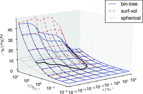
It is unsurprising that the models converge for high values of . This corresponds to instantaneous sintering (or coalescence) of particles upon collision. It is interesting to observe that for some combinations of the particles obtained through the binary tree model are larger; whereas for other combinations they appear smaller than the surface-volume model. Indeed, an intersection between these surfaces defines a line at which the particles obtained through both models are identical. This is shown in more detail in Figure 3, where the contours corresponding to the intersection of the binary tree and surface-volume models, and ±5% relative difference between the two are plotted. Specifically, the 5% error shading refers to the conditions under which:

Figure 3 FIG. 3 A contour plot depicting where the binary tree model is equivalent to the surface-volume model. The shading corresponds to within 5% deviation (with respect to collision diameter) of the surface-volume model from the binary tree model. (Color figure available online.)

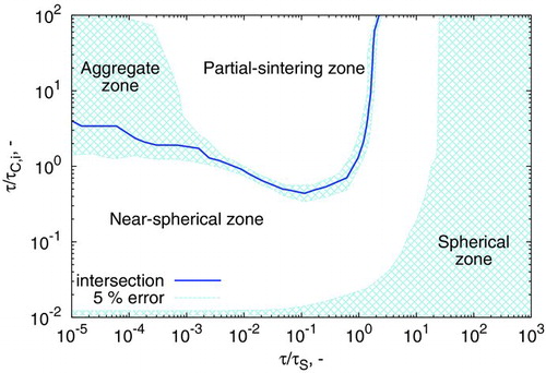
Four zones in this figure are identified, corresponding to different “types” of particles. Particles obtained in the spherical zone sinter sufficiently quickly to coalesce into spherical particles. In this zone, all particle models effectively reduce to the spherical particle model; and there is no benefit gained from tracking the additional structural detail of particles.

In the near-spherical zone, aggregates containing few primary particles are formed, either due to a fast sintering rate or a slow coagulation rate. Figure 2 illustrates that the particles predicted by the binary tree model have a larger collision diameter, corresponding to smaller primary particles. The reason for this can be understood by considering the derived properties of the particle models, in particular the expressions for collision diameter. It is shown in the online supplementary information, that, for coagulation of similarly sized particles, the surface-volume model will underestimate the predictions of the binary-tree model to a maximum of 10% difference. While this deviation is small, it causes potentially large changes in the rate of coagulation (rate in the free molecular regime), thus increasing the maximum error.

In the partial-sintering zone, particles coagulate to form partially sintered aggregates with more than two to three primary particles. Here, the surface-volume model overpredicts the results of the binary tree model. The reason for this can be understood by considering the sinterable surface area of an aggregate. As each connection node in the binary tree model is individually sintered (according to Equation (18)), there must always be more sinterable surface area in an aggregate described by the binary tree model than one described by the surface-volume model. This is mathematically demonstrated in the online supplementary information. If sintering occurs with the same characteristic time, the model with more sinterable surface area will sinter the particles faster (Equations (16) and (18)). In this case, this causes the binary tree model to predict the formation of smaller aggregates with larger primaries.

The intersection of the partial-sintering and near-spherical zones corresponds to the point where primaries are uniformly sized within an aggregate. As , the binary tree model becomes identical to the surface-volume model: aggregates are composed of unsintered monodisperse primary particles (the aggregate zone).

3.2. Effect of Polydispersity

The study in the previous section highlighted that under certain conditions, the surface-volume model yields aggregate particles with approximately the same size as the binary tree model. This, however, was determined for an initially monodisperse ensemble of particles (initial geometric standard deviation ). The purpose of this case study is to investigate how polydispersity can affect model performance, under conditions where the surface-volume and binary-tree models are equivalent for monodisperse particles. To investigate this, a point on the intersection line of Figure 3 was chosen (, τ/τ_C,i=5.0) and ensembles initialized with spherical particles of increasing polydispersity (up to ). The results are given in Figure 4.

Figure 4 FIG. 4 Effect of initial polydispersity,

, on morphology of particles. Shown are the normalized geometric mean

and standard deviation

of the collision and primary diameter. These were generated for

, τ/τ_C,i=5.0, on the “intersection” line of Figure 3. (Color figure available online.)

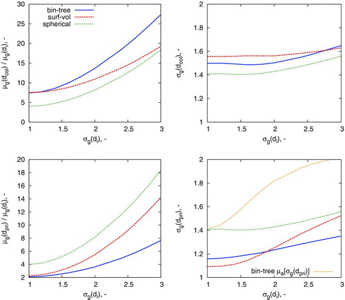
It is evident that the the surface-volume and binary-tree models perform comparably with . Under these conditions, there appears to be good agreement with the geometric mean collision and primary diameter and a small difference in geometric standard deviation of both. Beyond , the binary-tree model appears to predict larger aggregates with smaller primaries than the surface-volume model. This is attributed to the phenomenon discussed in Section 3.1 for the prediction of collision diameter in the near-spherical zone.

It is also interesting to observe that for the binary tree model, the standard deviation of the average primary diameter is significantly smaller than the average standard deviation of the primary diameter. This suggests that the local polydispersity within a particle can often be quite different to the polydispersity of the ensemble. The right panels of Figure 4 show that the spherical particle model yields ensembles with for . This indicates that the system has reached the self-preserving particle size distribution (Vemury and Pratsinis 1995).

In summary, this case study demonstrates that the prediction of the properties of an ensemble of polydisperse particles undergoing coagulation is strongly dependent on choice of the particle model. Highly polydisperse systems are poorly described by the spherical or surface-volume models where coagulation and sintering occur on similar timescales.

3.3. Computational Resources

While the binary tree model is capable of providing more information on particle structure and morphology, this comes at the cost of increased computational resources required. In order to capture all particle structure zones, a “slice” across Figure 3 at τ/τ_C,i=10 is taken, and the computational time required per run plotted in Figure 5. Calculations were conducted on an SGI Altrix Cluster with nodes composed of two 3.00 GHz quad-core Intel Harpertown processors and 8 GB of RAM.

Figure 5 FIG. 5 Comparison of computational time (

) required per run for τ/τ_C,i=10 to calculate τ=0.5 s of process time. (Color figure available online.)

Figure 6 FIG. 6 Comparison of model predictions for the silica system of Shekar et al. (2012a). Depicted are the zeroth moment (M₀), volume fraction (

), arithmetic mean (

), and geometric standard deviation (

) of the collision and primary diameters. (Color figure available online.)

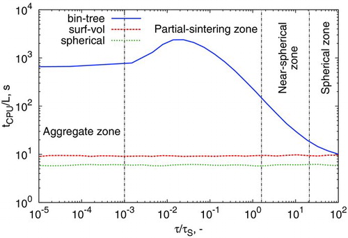
In the stochastic formulation of the population balance, it is evident that the surface-volume and spherical particle models require almost the same computational time, and this time is independent of the sintering rate. This is unsurprising, given that the additional effort required to adjust a particle’s surface area after a sintering event is minimal: it merely requires calculation of Equation (16).

The three models require the same computational time when spherical particles are obtained. Only when coagulation becomes important (relative to sintering) does the binary-tree model require more time, and in this case it requires orders of magnitude more. In the partial-sintering zone, particles containing more than one primary experience “merge” events, where two distinct primaries are combined into one due to sintering (Shekar et al. 2012a). These events alter the binary tree structure and as such, for large trees (i.e., particles with many primaries), more time is required to regenerate the tree structure after a node is lost. This phenomenon is responsible for the peak in computational time in the partial-sintering zone.

4. APPLICATION TO MODEL SYSTEMS

The case studies presented in the previous section were based on initialized ensembles of particles which could only undergo coagulation and sintering. However, in practical modeling applications, terms for inception, surface reaction, and condensation are also often included. This section presents two models in which quite different particle structures are obtained. For both studies, the characteristic coagulation time is estimated using the average properties of the ensemble: where m is the mass of an aggregate.

The expressions commonly encountered for the characteristic sintering time are highly nonlinear in diameter and temperature (Kobata et al. 1991; Buesser et al. 2011; Shekar et al. 2011; Menz et al. 2012). Thus, the three particle models will begin to diverge when sintering moves from effectively instantaneous (very small particles) to finite rate. The maximum primary particle diameter is therefore used to calculate the representative sintering time of the ensemble:

4.1. Silica Model

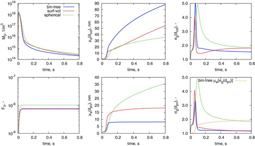
An adaptation of the binary-tree model to silica was presented by Shekar et al. (2012b). Further details of the model (including the form of its sintering characteristic time ) are given in the online supplementary information. Adapting the expressions in Shekar et al. (2012a) to the type-space of the surface-volume and spherical particle models, the temporal evolution of ensemble and particle characteristics is given in Figure 6.

Unsurprisingly, the spherical particle model performs poorly. This is to be expected given that the particles formed in this test system are aggregates. The surface-volume model is accurately able to capture the geometric standard deviation of the average estimated primary diameter . This is attributed to the physical narrowing of the primary particle size distribution due to sintering, as observed by Heine and Pratsinis (2007). The “spike” in geometric standard deviation in the major particle growth phase is due to simultaneous inception and coagulation and is consistent with previous modeling studies (Heine and Pratsinis 2007).

As noted in Section 3.2, it is possible that the use of across the particle ensemble may not fully capture the polydispersity of primaries in the aggregate. The slow increase of as opposed to the “spike” in indicates that the perceived polydispersity of the ensemble is quite different to that within an aggregate particle. This is potentially important structural information which cannot be resolved from surface-volume or spherical particle models.

The map of model performance as a function of amount of coagulation and sintering (Figure 3) is a useful tool in understanding where and why models begin to differ. It can also be applied to these specific modeling examples. As such, the movement of the particle ensemble with time t through the , space is plotted in Figure 7.

Figure 7 FIG. 7 Trajectory of the case of Shekar et al. (2012b) through the

,

space. The shading depicts the 5% error margins as described in Figure 3. Specific process times for the binary-tree and surface-volume models from Figure 6 are labeled. (Color figure available online.)

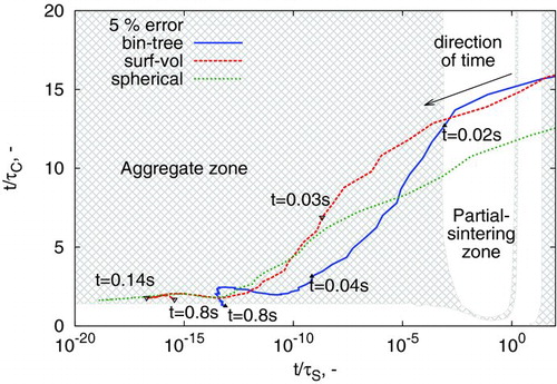
The very small values obtained for are associated with strong diameter dependence in the sintering time expression (Equation (S1), available in the online supplementary information). The near-spherical zone was therefore extrapolated from to account for this. The rapid movement across the space (as shown by the labeled times) is attributed to the fast growth of particles due to simultaneous surface reaction, coagulation, and sintering.

At early times, particles are spherical and in high number concentration. This causes the system to start in the “spherical zone,” at high values of . As particles grow, their characteristic sintering time increases. This causes a shift to lower values of . At the same time, the rate of coagulation slowly decreases, primarily due to the decrease in number density M₀. Finally, as the primary particle distribution becomes physically narrowed by sintering, the primary diameter ceases to change with time (Figure 6), allowing to steadily increase with increasing time t.

The models effectively separate paths once coagulation begins. This is evident in Figures 6 and 7, soon after the trajectories exit the spherical zone. Figure 7 also illustrates that even a very small amount of time spent in the near-spherical or partial-sintering zone can cause the predictions of surface-volume model to markedly deviate from those of the binary-tree model.

4.2. Silicon Model

The previous application focused on synthesis of aggregate particles, where coagulation and sintering are occurring on different timescales. It is, however, also common to attempt to model spherical or near-spherical particles (Wu et al. 1987; Backman et al. 2002; Körmer et al. 2010), where these two key processes can operate on similar timescales. An example of these conditions was recently identified in a multivariate model for silicon nanoparticle synthesis (Menz and Kraft 2013), where silicon particles were manufactured in a hot wall reactor at atmospheric pressure (Wu et al. 1987).

In this model, a grain-boundary diffusion sintering kinetic (Kobata et al. 1991; Kruis et al. 1993) is utilized. Further details regarding the model and its parameters are given in the online supplementary information. The evolution of important particle and ensemble characteristics for this model as applied to the case of Wu et al. (1987) is given in Figure 8. Note that a temperature profile (increasing from 500°C to 1250°C ) is imposed across this simulation (Wu et al. 1987; Nguyen and Flagan 1991; Menz and Kraft 2013).

Figure 8 FIG. 8 Comparison of model predictions for the case of Wu et al. (1987) using a multivariate silicon model (Menz and Kraft 2013). Depicted are the zeroth moment (M₀), volume fraction (

), arithmetic mean (

), and geometric standard deviation (

) of the collision and primary diameters. (Color figure available online.)

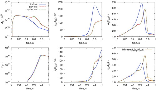
In this case, all models predict that spherical particles are obtained at the end of the process time. However, neither the surface-volume nor the spherical particle model perform comparably to the binary-tree model, with the number density M₀ double and average collision diameter 20% lower than that of the binary-tree model’s prediction. The surface-volume and spherical models predict the occurrence of a secondary nucleation period (at t=0.6 s in M₀ panel of Figure 9), consistent with other spherical particle modeling efforts (Nguyen and Flagan 1991) of this system.

The predictions of the surface-volume model are also very similar to those of the spherical particle model, despite containing a finite sintering rate. It is hypothesized that this is due to the high polydispersity of particles (, Figure 8 right panels) for this case study, resulting in a similar “convergence” of the two models as depicted in Figure 4. To further understand the differences between models here, this case is plotted atop Figure 3’s coagulation-sintering map in Figure 9.

Again, the system begins with small spherical particles at high t/τ_S. The three models diverge from each other after passing through the near-spherical zone. The surface-volume and spherical models subsequently show a large increase in coagulation rate, while it steadily decreases for the binary-tree model. This is due to the secondary nucleation period causing the number density to remain steady (Figure 8). The secondary nucleation period is absent for the binary tree model as the increased surface area of the aggregate particles causes faster depletion of the precursor.

Figure 9 FIG. 9 Trajectory of the case of Wu et al. (1987) using a multivariate silicon model (Menz and Kraft 2013) through the

,

space. The shading depicts the 5% error margins as described in Figure 3. Specific process times for the binary-tree and surface-volume models from Figure 8 are labeled, t<0.2 s omitted for clarity. (Color figure available online.)

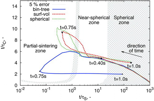
The minimum sintering rate reached at approximately 0.75 s represents the point at which the rate of decrease in sintering time is balanced by the contributions from the rate of increase in particle diameter and rate of increase in temperature. Past this point, the increasing temperature profile causes coalescence of aggregate structures, causing all models to return to the spherical zone. This case study highlights an example where experimental insight should be used with caution: if spherical particles are obtained experimentally, it does not necessarily justify the use of a spherical particle model.

5. CONCLUSIONS

This work has presented the mathematical formulation of particle models commonly used in aerosol dynamics of nanoparticles. A detailed numerical study was conducted in order to understand under which conditions these models differ. Starting from a set of identical conditions, the predictions of the resulting average properties of the particle ensemble were compared for each of the particle models. It was identified that under certain circumstances, all models were equivalent to a spherical particle model.

Outside of this range, the performance of the popular and computationally inexpensive surface-volume model with respect to a model which tracks full aggregate structure (binary-tree model) was evaluated. The two models gave alike results (to within a small error margin) where sintering was slow. However, where coagulation and sintering occurred on a similar timescale, the models predicted substantially different results. Further, the spherical and surface-volume particle models were shown to incur a large error margin where the coagulating ensemble was highly polydisperse.

The three models were also applied to modeling systems presented in earlier work. The first investigated aggregate formation where sintering primarily occurs on a much slower timescale than coagulation. Second, a model of silicon nanoparticle synthesis in which coagulation and sintering occur on approximately equal timescales was investigated. Here, it was evident that the additional structural information of the binary-tree model is essential in capturing the polydispersity of the ensemble and finite sintering kinetics of particles.

There is still considerable scope for further investigation of the behavior of particle models. Heterogeneous growth processes are well-documented contributors to rounding of particles (Lavvas et al. 2011; Shekar et al. 2012b) and have not been explicitly addressed in the present work. Further, only the most popular version of the surface-volume model has been used from among alternative two-dimensional formulations (Park and Rogak 2004; Heine and Pratsinis 2007) and different expressions for derived properties (Wells et al. 2006) exist.

As many population balance models use some degree of fitting or parameter estimation (Shekar et al. 2011; Menz et al. 2012; Chen et al. 2013), the error in use of a “simple” model will be reflected in the parameters obtained through the fitting procedure. The present work highlights that the choice of particle model does matter, and that a target modeling system should be well-characterized experimentally before proceeding to modeling.

[Supplementary materials are available for this article. Go to the publisher’s online edition of Aerosol Science and Technology to view the free supplementary files.]

Additional information

Notes on contributors

William J. Menz

William J. Menz acknowledges funding from the Cambridge Australia Trust to undertake this work. The authors additionally wish to thank the members of the Computational Modelling Group for their guidance and support. Markus Kraft gratefully acknowledges the DFG Mercator programme and the support of CENIDE at the Unviversity of Duisburg Essen.

Markus Kraft

William J. Menz acknowledges funding from the Cambridge Australia Trust to undertake this work. The authors additionally wish to thank the members of the Computational Modelling Group for their guidance and support. Markus Kraft gratefully acknowledges the DFG Mercator programme and the support of CENIDE at the Unviversity of Duisburg Essen.