Characterization of Dust Particles’ 3D Shape and Roughness with Nanometer Resolution

Abstract

Mineral dust particles in the atmosphere are often aspherical and their shape is important for a multitude of processes. Yet, measurements of the true shape in three dimensions are rare, even in a laboratory setting. Here, we employ atomic force microscopy to determine the 3D shape and surface roughness for two dusts commonly used in laboratory experiments, Arizona test dust (ATD) and kaolinite. Our major finding is that both are thin and remarkably smooth. An oblate spheroidal description is an excellent fit to these data. We use correlation analysis to further examine the surface properties of the dusts and find essentially no features at horizontal spatial scales between ∼10 and 100 nm. This surprising result is supported by the agreement between our specific surface area and BET surface area measurements. The thin, smooth, spheroidal approximation has many implications for physical processes in the atmosphere, including dust transport and radiative transfer.

Copyright 2015 American Association for Aerosol Research

1. INTRODUCTION

Mineral dust is the most abundant solid aerosol particle by mass in Earth’s atmosphere; between one and three thousand Tg are emitted each year (Cakmur et al. 2006). Once aloft, the dust scatters and absorbs solar and terrestrial radiation, thus playing a role in Earth’s net radiative balance. Dust particles also catalyze cloud formation at low supersaturations, acting as so-called giant cloud condensation nuclei (van den Heever et al. 2006); at temperatures below water’s melting point, they can initiate freezing (Hoose and Möhler 2012). Dust is also an important surface for chemical reactions in the atmosphere (Usher et al. 2003; Formenti et al. 2011; Harris et al. 2013) and is an important nutrient in the open ocean (Schulz et al. 2012).

The extent to which dust particles affect processes in Earth’s atmosphere is, in large part, governed by their lifetime. Large particles typically settle out of the atmosphere quickly, close to the region in which they are emitted. Smaller particles can be transported much further, across oceans in some cases (Abouchami et al. 2013; Liu et al. 2013). While particle size is usually the dominant effect in determining a particle’s fall speed, the shape will also play a role (Ginoux 2003). For a given mass, aspherical particles have a greater surface area, and therefore greater drag, which reduces their fall speed (Yang et al. 2013).

Knowing the shape of dust particles is thus important in determining their lifetime in the atmosphere. Shape also affects the ways in which dust particles interact with radiation. A study of the radiative effects of Saharan dust showed that up to a 55% change in the solar plus thermal forcing over ocean surfaces was attributable to particle asphericity (Otto et al. 2011). Recent detailed laboratory investigations have also shown that the shape of particles, as well as their mineralogy play an important role in the ways in which they interact with infrared and visible radiation (Hudson et al. 2008a,b). The investigators were able to model complex mixtures of mineral dusts more accurately by including the shape of the particles (Laskina et al. 2012). In particular, using shapes that included more eccentric spheroids improved the agreement between the measured and modeled spectra of the dusts (Alexander et al. 2013).

Despite its importance, measurements of the three-dimensional shape of mineral dust particles remain scarce. In fact, a recent paper included the following in the final section, “Synthesis and recommendations”: “Data on the third dimension of particles and the surface roughness are very rare but are needed for optical modeling” (Formenti et al. 2011). There are many techniques which capture some aspect of particle size, but most are based on an assumption that the particles in question are spheres. For example, optical particle counters are sensitive to an orientational average of the three-dimensional shape of particles within the sensing volume, but the reported “size” is the diameter of a sphere with the same scattering signal. Similarly, the “size” from a scanning mobility particle sizer (SMPS) is derived from a balance between an electrical force, which is shape-independent, and drag, which varies with shape. The reported diameter is that of a sphere with the same electrical mobility as the particle in the analyzer.

One way to quantify the complicated morphology of mineral dust particles is to analyze the detailed images acquired via scanning electron microscopy (SEM), though such images are inherently two-dimensional. Departures from circularity are easily seen in the dimensions parallel to the collecting substrate, but the height of the particle is highly uncertain (Reid et al. 2003). In an effort to derive, for example, the volume of dust from SEM images, an assumption is usually made as to a relationship between the projected area of the particle and its height. Most frequently, the cross-sectional area is approximated as an ellipse, and the minor axis is assumed as the height of the particle (Reid et al. 2003; Kandler et al. 2009).

Such an assumption may dramatically overestimate the height of the particle. Okada et al. (2001) collected samples of dust from three arid regions in China, and estimated the height of the particles by analyzing the shadow angle after coating the particles with a Pt/Pd alloy at an angle of 26.6°. The mean height of the particles ranged from 60 to 40% of their maximum length with extreme values reaching only 5–10% of the maximum length. More recently, Veghte and Freedman (2014) analyzed particles using a tilted SEM stage, allowing them to access the height of the particles, as well as the projected area. Clay minerals (illite, kaolinite, and montmorillonite) were thin, with aspect ratios ranging from five to nine, while calcite and quartz were more compact, with mean aspect ratios between unity and two. Motivated specifically by the desire to acquire information on particles’ volume and actual surface area, Barkay et al. (2005) collected samples from over Crete and analyzed them with an Atomic Force Microscope (AFM) as well as SEM. The AFM directly probes a sample’s three-dimensional topography, thus enabling a true measure of volume and a closer representation of a particle’s surface area. (See the following text for a more complete discussion of this point.) They found that many particles were well described as disks with a height as much as 10 times smaller than the diameter of the base. Gwaze et al. (2007) and Chou et al. (2008) also found that the height of the particles they analyzed was substantially less than any measure of the size of the projected area.

As little as is known of the true three-dimensional shape of aerosol particles, even less is known of the details of the surface roughness, which is relevant for light scattering, chemical reactions, and (perhaps) catalysis of phase transitions (Formenti et al. 2011; Hoose and Möhler 2012). Even defining surface roughness can be problematic. After all, what might be considered roughness for one application would be considered part of the overall shape in another.

Qualitatively, surface roughness is apparent in many images acquired with an SEM, but quantitative analysis of such images is difficult because brightness in the SEM image is a convolution of tilt/curvature and the chemical composition of the sample. Atomic force microscopy is a natural tool for analysis of surface roughness, but the procedures for acquisition of the AFM images are not as well developed as those for SEM analysis. However, limited AFM analysis of dust particles by Chou et al. (2008) revealed that particles were remarkably smooth (see Chou et al.’s Figure 8). Similarly, Helas and Andreae (2008) also found that Saharan dust particles were smooth; the surface roughness was not quantified in either case.

In this article we analyze two mineral dusts commonly used in laboratory experiments as surrogates for atmospheric dusts—Arizona test dust (ATD; Powder Technology, Inc.) and kaolinite (Fluka) (Bedjanian et al. 2013; Glen and Brooks 2013; Rubasinghege et al. 2013; Wright and Petters 2013; Welti et al. 2014). We employed both scanning electron and atomic force microscopy to derive the particles’ shapes and surface roughness. In the following section, we outline the procedures used for both data acquisition and analysis, including our protocols for acquiring the AFM images of the dust particles. We discuss the overall shape of the two dusts and their surface roughness and conclude with implications of these findings for dusts in the atmosphere.

2. METHODS AND DATA ANALYSIS

2.1. AFM

In order to study the dusts via atomic force microscopy, the particles must be immobilized upon the substrate to prevent the AFM tip from dragging them during imaging. We employed two sample preparations. The first was to deposit water mixed with dust on mica (Tarheel Mica Co.). After the water evaporates, the sample is ready to use (Macht et al. 2011). We expect that slightly soluble components in dust would dissolve in water and, as the water evaporates, partially cement the particles onto the mica. The other sample preparation was to first deposit a layer of Superglue™on mica, then deposit a small quantity of dust on it while the glue was still wet. The dust particles settled lightly onto the glue and were held in place once it dried (usually two to three days). We saw no difference in the AFM images of the dusts dispersed in water versus those dispersed in air onto the glue.

The measurements with the atomic force microscope were made with a Nanosurf Easyscan AFM in the tapping mode, which was employed to minimize the chance that the particles moved during imaging. If a particle did move, the image had obvious discontinuities and was rejected on that basis. We used a T-190R-10 cantilever (Nanoscience Instruments) which is 225 μm long with a spring constant of 48 N/m. The tip is pyramidal with a radius at the apex less than 10 nm; they are typically 14 μm in height.

The cantilever tip contact with sample was 2048 times per line; each line scan took 2–3 s. The images we acquired are 9–625 μm² with a vertical resolution of 0.37 nm. With an infinitely thin AFM tip, our horizontal resolution would be the lateral dimension of the image divided by the number of times the tip interacted with the surface. For the numbers given above, that is 5–25 nm. In practice, of course, the tip has a finite size, which decreases the resolution (Haugstad 2012, pp. 180–181). For our tips, which have a radius of ∼8 nm (guaranteed by the manufacturer less than 10 nm), the resolution is ≈12 nm. Note that the accuracy of the measurement in the vertical direction is a function of the horizontal separation of features. The AFM probe cannot access deep, narrow crevices and cannot accurately image narrow thin spikes because of the finite size of the probe tip. We expect neither case for the particles we image here.

Because the particles cannot be detected optically, we simply scanned an area of the substrate, then looked for particles within the image using the Nanosurf software. Once particles were identified, they were isolated and exported for further analysis using MatLab™.

To facilitate quantitative analysis of the images, we first corrected the slope of the background for each individual particle and then set the background to zero. After that procedure, the contour, which is the edge of the particle’s projected area, was readily apparent.

The longest distance between two points on the contour is the maximum length, L_max. The area-equivalent diameter, D_aeq, is defined through the relation[1] where A_p is the particle’s projected area. For spherical particles, L_max = D_aeq.

The maximum height, h_max, is the distance between the highest point of the particle to zero. The volume, V, is defined as[2] where s is the lateral distance between adjacent points and h_i is the height (above baseline) of the i^th point in the image. The surface area of the portion of the particle detected by the AFM, S_m, is derived from the h_i by approximating the surface as tesselated triangles. Given the three vertices (i.e., the h_i), we calculated the area of the triangles using Heron’s formula. The surface area which we use in subsequent analyses is then[3] we add A_p to account for the portion of the particle that the AFM cannot access.

This is, of course, not the actual surface area of the particles because of the AFM’s finite horizontal resolution and any curvature that the particles have. Figure 1 illustrates this for an oblate spheroid, which is typical for our particles. The “x”s in the schematic denote an interaction of the AFM with the particle. As the top view shows, a finite resolution distorts the shape of the particle as shown by the dashed line. With finer resolution, the particle’s true shape is recovered.

FIG. 1. Schematic illustrating the uncertainty in a particle’s area as measured by atomic force microscopy. The “x”s denote an interaction of the AFM with the particle, which is an oblate spheroid. The solid line is the particle’s actual shape, the dashed line is the shape as inferred from the AFM data. With higher resolution, the particle’s projected area is recovered; however, the area from Equation (3[3] ) is greater than the actual surface area, even in the case of infinite resolution, because of the particle’s curvature on the underside.

Though the particle’s projected area can be recovered in the limit of infinite resolution, the true surface area cannot be because of the curvature that the AFM cannot access (i.e., the curvature on the bottom of the particle). In essence, a particle such as the one shown in the figure appears to be sitting on a pedestal or plinth, with only the top half of its surface truly represented. The lower panel in the figure shows that the surface area as determined by the AFM is always greater than the true surface area, as long as the inaccessible curvature is positive. We estimate that the surface area, as determined using Equation (3[3] ), may be greater than the true surface area by as much as 11%.

We conclude this section with the caveat that though curvature on the underside of a particle (i.e., the portion not accessible to an AFM) is possible, it is not required. Inspection of side-view SEM images of mineral dust particles shown in Veghte and Freedman (2014) show that many of them are lying flat on the substrate. If imaged with an AFM, no dramatic discontinuity marking the particle’s edge would be evident.

2.2. Analysis of Particle Roughness

While it is relatively straightforward to define and characterize roughness for a flat surface, for our particles, shape and roughness must be separated. Because there is not a universal algorithm to describe particles’ roughness, we characterized it in a couple of ways, using different perspectives to highlight different aspects of roughness. As a first look, we numerically smoothed the particle, then compare the smoothed surface areas to the original. The surface area of rough particles will decrease substantially upon smoothing while particles which are already smooth will change very little.

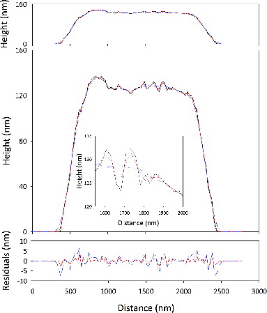
The numerical smoothing is with a lowess filter, which employs a locally weighted linear regression. In this way, the overall shape is preserved. The size of the smoothing window in the lowess filter determines the scale of the feature which shows up as roughness. Features with sizes much bigger than the smoothing window are effectively part of the particle’s overall shape. For example, consider the data from one of the ATD particles, shown in Figure 2. The overall shape of the particle is preserved, but the smaller features, for example those near the particle’s maximum height are smoothed. The dashed line (red) in the inset is the smoothed data for a smoothing window of five points; the scale of roughness probed is small as the smoothed particle is very much like the original. In contrast, a wider smoothing window, shown as the dash-dot line (blue) in the figure preserves the overall particle shape, but highlights features between 1600 and 1900 nm as roughness now.

FIG. 2. Shape vs. roughness: as the top panel shows, particles are thin and remarkably smooth. The middle panel is a repeat of the data in the top one with an expanded vertical scale so that the particle’s roughness (such as it is) can be seen. The inset to the middle panel illustrates the amplitude of the deviations from the overall particle shape. The inset also highlights the interplay between overall shape and roughness. Raw data are shown as a solid line (black). A smoothed version of the raw data is regarded as shape while deviations from it are roughness. The lower panel shows the residuals by subtracting the raw data from the mean shape defined by the smoothing procedure. The deviations from the particle shape do not exceed a few nanometers, reinforcing the point that the particles are smooth, at least on the scales chosen here.

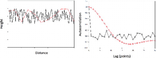
One traditional measure of roughness is the root-mean-square deviations of raw data from a mean (or smoothed version of the data). One weakness in that approach is that the characteristic horizontal length scale is unspecified. As the horizontal length scale increases, the profile appears progressively smoother though the rms deviations can be the same.

An example is shown in Figure 3. Here, we generate artificial profiles by adding random numbers to a mean height of 1.0. (Note that the units are arbitrary in this example.) The rms roughness of both profiles in Figure 3 is the same though the dashed line (red) appears to be the smoother of the two. That, however, is simply because the horizontal scaling of the vertical deviations from the mean is expanded. (In fact, the dashed line [red] is simply the first 11 points of the solid line [black]. That data are stretched horizontally and re-sampled such that the two traces have the same horizontal resolution.) The autocorrelations, shown in the lower panel of Figure 3, reveal the scale of the roughness. The autocorrelation for the data shown as the solid line (black) in the upper panel drops to approximately zero within one lag. There are no persistent structures or features at scales larger than the resolution. In contrast, the autocorrelation for the data shown in the upper panel as the dashed line (red) drops to zero only after approximately 10 lags. The autocorrelation reveals that there are features approximately 10 times larger than the resolution.

FIG. 3. An example of using the correlation length to quantify the size of surface features. Example profiles are shown in the top panel with the corresponding autocorrelation functions in the lower panel.

Using this analysis, we quantify the horizontal length scale of the particles’ surface roughness by first smoothing the particle with a lowess filter using a specified smoothing window, then subtracting the smoothed data from the original. We then compute the autocorrelation function of the residuals. Examples of the residuals from the two smoothing procedures described earlier are shown in the lower panel of Figure 2. In neither case, do the residuals exceed 10 nm, reinforcing our assertion that the particles are, in general, quite smooth.

2.3. SEM

Aerosol particles analyzed via Scanning Electron Microscopy were dispersed with a fluidized bed (TSI, 3400A), then collected on 13-mm diameter Nuclepore clear polycarbonate filters with a pore size of 0.1 μm (Whatman Inc., Chicago, IL, USA) mounted in Costar Pop-Top membrane holders. The sample flow was split before the membrane filter and the second line was connected to a condensation particle counter (CPC, TSI 3772) to monitor the aerosol concentration. After the particles had been collected, the filters were mounted on aluminum stubs and coated with a 1.6-nm Pt/Pd alloy layer using a Sputter coater (Hummer™ 6.2) for scanning electron microscopy analysis. The coated filters were imaged using an Hitachi S-4700 field emission scanning electron microscope.

SEM micrographs of dust particles were processed using the freely available ImageJ software (National Institutes of Health). High magnification images of dust particles were used to estimate morphological parameters. Each particle was individually processed and thresholds were adjusted to convert the image into a binary image. The parameters calculated from the binary images were the maximum projected length, L_max, which is the distance between the most separated points in the projected image, and the total projected area of the particle, A_p.

3. RESULTS

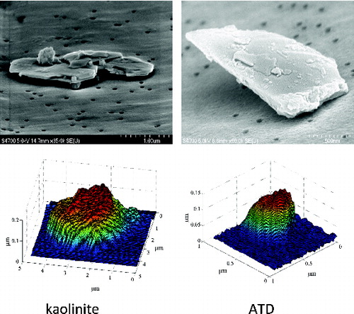
As discussed in the previous section, both SEM and AFM data were used for our analysis; they both have advantages. We have a large quantity of accurate SEM data which shows two dimensions of the dust particle clearly. Acquisition of the AFM data is more time consuming, but it shows the detailed, three-dimensional structure which the SEM does not. Figure 4 shows examples of SEM and AFM images for kaolinite and ATD.

FIG. 4. Examples of SEM (top row) and AFM (bottom row) images of kaolinite (left column) and ATD (right column). Note that it was not possible to image the same particles with both SEM and AFM. The images in the figure are of four different particles. The SEM images were taken with a tilted sample stage, which enables an estimation of the particle’s thickness in some cases. Note that the vertical and horizontal scales are different in the AFM images.

3.1. Shape

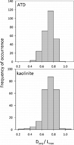
From the SEM data, we see that the particles are rather round, in agreement with previous studies. Figure 5 shows that the ratio for both ATD and kaolinite. We were able to analyze particles with the SEM as a function of mobility diameter and found no dependence of on the mobility diameter (data not shown). Analysis of the cross-sectional area as seen by the AFM yields for the ATD and for the kaolinite. (The uncertainty here is the standard deviation; the different precisions used earlier reflect differing standard deviations in the distribution of the ratio .)

FIG. 5. Histograms of the ratio from SEM data. Both ATD and kaolinite have a ratio of 0.7 0.1. In both cases, the particles’ projected areas are close to circular.

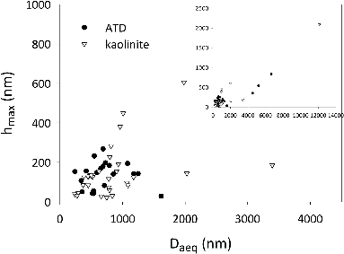
In addition to the shape of the cross-section, the AFM data reveal that the height of the particle is small compared to the horizontal scale, as shown in Figure 6. The maximum height of the particles is an order of magnitude smaller than . Taken together, Figures 5 and 6 suggest that Arizona test dust and kaolinite are well-modeled as disks or oblate spheroids with a polar to equatorial axis ratio .

FIG. 6. Maximum height, , as a function of from the AFM data. is typically an order of magnitude smaller than ; the ratio, , does not vary by size. The inset to the figure shows the full range of and that we measured.

As a test of that assertion, we calculated the surface area of oblate spheroids, using as the equatorial radius and as the polar radius, and compared those values with , calculated using Equation (3[3] ). For ATD, the ratio while for kaolinite . The close agreement between the calculated and the measured surface area lends strong support to the smooth, oblate spheroid approximation. This has numerous implications for remote sensing of dust (among other things), as discussed in the concluding section.

3.2. Roughness

Our data show that kaolinite and Arizona test dust are rather smooth, oblate spheroids. We know, however, that the particles are not perfectly smooth. For example, there are clearly residuals in Figure 2, remaining after smoothing a particle profile with a lowess filter. To further quantify the particles’ roughness, we first numerically smoothed them, calculated the new surface area, and then compared the new value with the original. The result of two such approaches is shown in Figure 7.

FIG. 7. Ratio of the smoothed to original surface area of ATD and kaolinite particles as they are numerically smoothed. The upper panel shows the change in the surface area upon smoothing the particles repeatedly with a five-point lowess filter. The lower panel shows the change as the particles are smoothed with a filter of varying size. In both cases, the change in surface area is minimal (less than 2%), supporting our previous assertion that the particles are smooth.

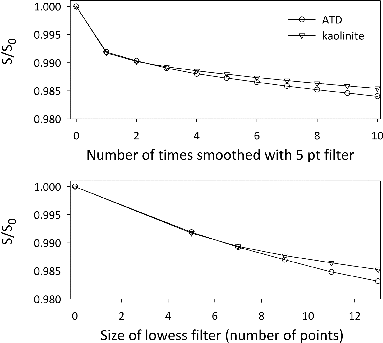
We first repeatedly smoothed the data with a five-point lowess filter, shown in the upper panel of Figure 7. The surface area decreases by less than 1% upon smoothing the data one time. Eight more smoothing operations resulted in another 1% decrease in the surface area. Such small changes show that the particles are very smooth to begin with. If they were rough (on that scale), successive smoothing operations would result in a much larger decrease in the surface area.

As a first attempt at characterizing the scale of the surface roughness, we varied the size of the window in the lowess filter from 5 to 13 points, shown in the lower panel in Figure 7. The size of the window dictates the size of the particles’ features which are identified as roughness. As expected, the surface area decreased as the size of the smoothing window increased. Larger and larger features, previously captured as the overall shape of the particle, were identified as roughness and smoothed. Though the surface area did continue to decrease as the size of the smoothing window was increased, the decrease was minimal, indicative of particles which are relatively smooth at both large and small scales.

As a further quantification of the surface roughness, consider Figure 8, which shows histograms of the residuals after smoothing for ATD (left) and kaolinite (right) as well as plots of the autocorrelation function (bottom row). The histograms are a further quantification of our assertion that the particles are smooth. The magnitude of the residuals for both types rarely exceeds 2 nm, though as expected, the distribution of residuals broadens as the smoothing window is increased. These histograms also exhibit one of the few differences we see between the dusts—the kaolinite has a broader distribution for all smoothing windows.

FIG. 8. Histogram of the residuals (top row) for ATD (left) and kaolinite (right). The residuals are the results of subtracting smoothed data from the original after using 5, 11, and 15-point lowess filters corresponding to smoothing ranges of 60, 132, and 180 nm. Only particles which were measured with a resolution of nm are included in this analysis. The magnitude of the residuals sets the vertical scale of the roughness. The mean autocorrelation of the residuals (bottom row) for ATD and kaolinite provides the horizontal scale of the roughness.

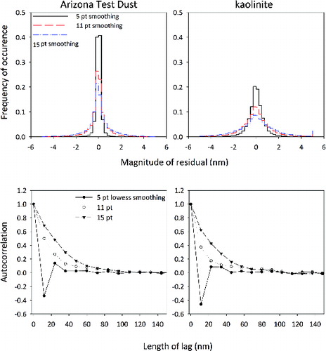
The magnitude of the residuals shows the vertical scale of the particles’ roughness, but does not show the horizontal scale over which those deviations occur. The autocorrelation function is frequently used in the analysis of surface roughness in the context of scattering, as not only the deviations from the mean but also the scale over which those deviations occur is important (Bennett and Mattson 1989; Ogilvy 1991). For both dusts, the autocorrelation of the residuals remaining after smoothing with a five-point filter decays to zero within two lags (i.e., twice the resolution), strongly suggesting that there are few features present at that scale. In contrast to the residuals from the five-point lowess filter, those from the 11- and 13-point filter decay to an autocorrelation of zero much more slowly. There are features smaller than 132 and 180 nm, not captured as the overall shape of the particle, which contribute to the residuals, appearing as roughness. The autocorrelation persists for approximately five to eight lags, consistent with feature sizes of 100 nm.

Figure 8 suggests that both Arizona test dust and kaolinite are smooth below a scale of about 100 nm, which may seem surprising. Dust is typically regarded as rough, providing sites for chemical reactions (Underwood et al. 2001) and ice nucleation (Hoose and Möhler 2012). The surface area available for such small, molecular-level processes can be quantified via the the BET surface area, which is measured via adsorption of nitrogen onto the particles’ surfaces (Brunauer et al. 1938). The BET surface area typically exceeds the area computed from electrical mobility measurements, for instance, by a factor of 10 or more. We can compare our surface area measurements to those derived from BET measurements by converting our volume measurements to mass. Using a density of 2.65 g/cm for ATD (Wagner et al. 2008), we arrive at a surface area density of 4.4 m/g. A similar analysis for kaolinite yields a specific surface area of 10.2 m/g.

Wagner et al. (2008) cite a BET surface area for Arizona test dust of 5.7 m/g, 130% of our value. The agreement between that and our specific surface area supports the conjecture that the surface area of ATD is dominated by features with a scale greater than 10 nm, the resolution of our measurements for the roughness analysis. Similarly, Bickmore et al. (2002) cite a range of BET surface area values for kaolinite, from eight to 20 m/g, depending upon the source of the kaolinite. (All of the samples that they reference were obtained from the Clay Mineral Society.) The fact that our specific surface area falls within that range also supports the assertion that the features which dominate the surface area of the kaolinite dust are 10 nm in size or greater.

A more recent comparison of the surface area measured via atomic force microscopy and BET adsorption isotherms showed a substantial discrepancy between the two. Macht et al. (2011) found that the specific surface area as measured by an AFM was a factor of two to five times greater than that derived from BET measurements. They attributed the difference to delamination of the minerals (illite and montmorillonite) during dispersion in an NaOH solution and subsequent sonication.

4. IMPLICATIONS FOR THE ATMOSPHERE AND CONCLUDING REMARKS

The finding that these particles are thin, smooth oblate spheroids has numerous implications for such particles in the atmosphere. As noted in the Introduction, these include gravitational settling, radiative transfer, and chemical reactions. For example, the asphericity of particles can enhance forward scattering and reduce backscattering, thereby making the extinction coefficient and single-scattering albedo different from the spherical value. Hence, particle shape must be considered in dust radiative forcing calculations and included in climate models.

In the often-used special case of optically large randomly oriented particles, smoothness and convexity of the particles allows for great simplification in scattering calculations via the so-called Cauchy’s Theorem. The theorem states that in the geometrical optics limit, the orientation-averaged extinction cross-section equals one quarter of the surface area (Krotkov et al. 1999). Hence, at a given volume, spheres scatter least and our findings of large aspect ratios for ATD and kaolinite imply greater scattering per unit mass than in the spherical case. Furthermore, for optically small particles, it turns out that spheres still scatter the least as was recently elaborated in Kostinski and Mongkolsittisilp (2013) where it was shown that orientation-averaged dipole moment of a sphere is below that of volume-equivalent spheroids and the dependence is monotonic with the aspect ratio. Insofar as most satellite retrievals of transported dust mass, etc., rely on the optical depth (), the effect of suspended dust particle shape on is just as pronounced and can therefore also lead to errors if the large-aspect oblate spheroidal shape is ignored.

Particle shape affects air resistance as well and can influence, e.g., the vertical distribution of dust during transatlantic transport. Because of higher drag, at a given volume and mass, aspherical particles fall more slowly and hence stay aloft longer than their spherical analogues. This is particularly pronounced for settling at low Reynolds numbers (Stokes regime, relevant to the micron-sized particles studied here). In this regime, an irregularly shaped particle will experience a drag similar to a circumscribing sphere with the diameter of the particle’s longest dimension (Guyon et al. 2001). (This striking fact is related to the Stokes paradox [Birkhoff 1960].) As a result, for a given mass, residence time in the troposphere is greatly increased. Computing the diameters of the equivalent spheres from our volume measurements, and writing , we find that . Since , . These oblate spheroids settle at only 22% of the velocity as spheres of the same volume. Such effects may lead to shape stratification in a vertical column of suspended dust and may be detected remotely via lidar depolarization measurements, e.g., Yang et al. (2013).

Shape and roughness also play a role in chemical reactions upon mineral dust particles. Many ice nuclei in the atmosphere are composed primarily of mineral dust, and surface roughness of that dust has been hypothesized as a contributor to the fact that some dusts seem to be much more effective than others (Hoose and Möhler 2012). The available area for chemical reactions upon dust also depends upon surface roughness. Our measurements and the comparison to the available BET measurements suggest that surface area from features with scales below 10–20 nm contributes only an additional 30–40%, at least for Arizona test dust and kaolinite. (Dusts with micropores [e.g., zeolites] could be a significant exception to this.)

In summary, Arizona test dust and kaolinite, two popular proxies for atmospheric dusts used in laboratory experiments, are well-approximated as smooth, oblate spheroids with an equatorial to polar axis of approximately eight. Such a model has implication for radiative transfer, transport, and chemical reactions upon the dust.

ACKNOWLEDGMENTS

Thanks to John Jaszczak who provided us with access to the AFM and provided advice on getting started.

FUNDING

This work was funded through National Science Foundation grants AGS-1028998, AGS-1039742, and AGS-1119164.

REFERENCES

- Abouchami, W., Näthe, K., Kumar, A., Galer, S. J. G., Jochum, K. P., Williams, E., et al. (2013). Geochemical and Isotopic Characterization of the Bodélé Depression Dust Source and Implications for Transatlantic Dust Transport to the Amazon Basin. Earth Planetary Sci. Lett., 380: 112–123.
- Alexander, J., Laskina, O., Meland, B., Young, M. A., Grassian, V., and Kleiber, P. (2013). A Combined Laboratory and Modeling Study of the Infrared Extinction and Visible Light Scattering Properties of Mineral Dust Aerosol. J. Geophys. Res., 118: 435–452.
- Barkay, Z., Teller, A., Ganor, E., Levin, Z., and Shapira, Y. (2005). Atomic Force and Scanning Electron Microscopy of Atmospheric Particles. Microsc. Res. Tech., 68(2): 107–114.
- Bedjanian, Y., Romanias, M. N., and El Zein, A. (2013). Interaction of OH Radicals with Arizona Test Dust: Uptake and Products. J. Phys. Chem. A., 117(2): 393–400.
- Bennett, J., and Mattson, L. (1989). Introduction to Surface Roughness and Scattering. Optical Society of America, Washington, DC.
- Bickmore, B. R., Nagy, K. L., Sandlin, P. E., and Crater, T. S. (2002). Quantifying Surface Areas of Clays by Atomic Force Microscopy. Am. Mineral., 87(5–6): 780–783.
- Birkhoff, G. (1960). Hydrodynamics: A Study in Logic, Fact and Similitude. Princeton University Press, Princeton, NJ.
- Brunauer, S., Emmett, P. H., and Teller, E. (1938). Adsorption of Gases in Multimolecular Layers. J. Am. Chem. Soc., 60(2): 309–319.
- Cakmur, R. V., Miller, R. L., Perlwitz, J., Geogdzhayev, I. V., Ginoux, P., Koch, D., et al. (2006). Constraining the Magnitude of the Global Dust Cycle by Minimizing the Difference Between a Model and Observations. J. Geophys. Res Atmos., 111( D6):D06207; DOI: 10.1029/2005JD005791.
- Chou, C., Formenti, P., Maille, M., Ausset, P., Helas, G., Harrison, M., et al. (2008). Size Distribution, Shape, and Composition of Mineral Dust Aerosols Collected During the African Monsoon Multidisciplinary Analysis Special Observation Period 0: Dust and Biomass-Burning Experiment Field Campaign in Niger, January 2006. J. Geophys. Res., 113( D23):D06207, DOI: 10.1029/2008JD9897.
- Formenti, P., Schtz, L., Balkanski, Y., Desboeufs, K., Ebert, M., Kandler, K., et al. (2011). Recent Progress in Understanding Physical and Chemical Properties of African and Asian Mineral Dust. Atmos. Chem. Phys., 11(16): 8231–8256.
- Ginoux, P. (2003). Effects of Nonsphericity on Mineral Dust Modeling. J. Geophys. Res. Atmos., 108( D2):4052, DOI: 10.1029/2002JD002516.
- Glen, A., and Brooks, S. D. (2013). A New Method for Measuring Optical Scattering Properties of Atmospherically Relevant Dusts Using the Cloud and Aerosol Spectrometer with Polarization (CASPOL). Atmos. Chem. Phys., 13(3):1345–1356, WOS:000315406100016.
- Guyon, E., Hulin, J., Petit, L., and Mitescu, C. (2001). Physical Hydrodynamics. Oxford University Press, Oxford.
- Gwaze, P., Annegarn, H. J., Huth, J., and Helas, G. (2007). Comparison of Particle Sizes Determined with Impactor, AFM and SEM. Atmos. Res., 86(2): 93–104.
- Harris, E., Sinha, B., Pinxteren, D. v., Tilgner, A., Fomba, K. W., Schneider, J., et al. (2013). Enhanced Role of Transition Metal Ion Catalysis During In-Cloud Oxidation of SO2. Science., 340(6133): 727–730.
- Haugstad, G. (2012). Atomic Force Microscopy. John Wiley & Sons, Hoboken, NJ.
- Helas, G., and Andreae, M. O. (2008). Surface Features on Sahara Soil Dust Particles Made Visible by Atomic Force Microscope (AFM) Phase Images. Atmos. Meas. Tech., 1(1): 1–8.
- Hoose, C., and Möhler, O. (May 2012). Heterogeneous Ice Nucleation on Atmospheric Aerosols: A Review of Results from Laboratory Experiments. Atmos. Chem. Phys. Discuss., 12(5):12531–12621.
- Hudson, P., Gibson, E., Young, M., Kleiber, P., and Grassian, V. (2008a). Coupled Infrared Extinction and Size Distribution Measurements of Several Clay Components of Mineral Dust Aerosol. J. Geophys. Res., 113( D01201), doi:10.1029/2007JD008791.
- Hudson, P., Young, M., Kleiber, P., and Grassian, V. (2008b). Coupled Infrared Extinction and Size Distribution Measurements of Several Non-Clay Components of Mineral Dust Aerosol (Quartz, Calcite, and Dolomite). Atmos. Environ., 42: 5991–5999.
- Kandler, K., Schtz, L., Deutscher, C., Ebert, M., Hofmann, H., Jckel, S., et al. (2009). Size Distribution, Mass Concentration, Chemical and Mineralogical Composition and Derived Optical Parameters of the Boundary Layer Aerosol at Tinfou, Morocco, During SAMUM 2006. Tellus B., 61(1): 32–50.
- Kostinski, A. B., and Mongkolsittisilp, A. (2013). Minimum Principles in Electromagnetic Scattering by Small Aspherical Particles. J. Quant. Spec. Rad. Tran., 131: 194–201.
- Krotkov, N. A., Torres, O., Seftor, C., Krueger, A. J., Kostinski, A., Rose, W. I., et al. (1999). Comparison of TOMS and AVHRR Volcanic Ash Retrievals from the August 1992 Eruption of mt. spurr. Geophys. Res. Lett., 26(4): 455–458.
- Laskina, O., Young, M., Kleiber, P., and Grassian, V. H. (2012). Infrared Extinction Spectra of Mineral Dust Aerosol: Single Components and Complex Mixtures. J. Geophys. Res., 117, doi:10.1029/2012JD017756.
- Liu, Z., Fairlie, T. D., Uno, I., Huang, J., Wu, D., Omar, A., et al. (2013). Transpacific Transport and Evolution of the Optical Properties of Asian Dust. J. Quant. Spectrosc. Radiat. Transf., 116: 24–33.
- Macht, F., Eusterhues, K., Pronk, G. J., and Totsche, K. U. (2011). Specific Surface Area of Clay Minerals: Comparison Between Atomic Force Microscopy Measurements and Bulk-Gas (n2) and -Liquid (EGME) Adsorption Methods. Appl. Clay Sci., 53(1): 20–26.
- Ogilvy, J. (1991). Theory of Wave Scattering from Random Rough Surfaces. Adam Hilger, Bristol, UK.
- Okada, K., Heintzenberg, J., Kai, K., and Qin, Y. (2001). Shape of Atmospheric Mineral Particles Collected in Three Chinese Arid-Regions. Geophys. Res. Lett., 28(16): 3123–3126.
- Otto, S., Trautmann, T., and Wendisch, M. (2011). On Realistic Size Equivalence and Shape of Spheroidal Saharan Mineral Dust Particles Applied in Solar and Thermal Radiative Transfer Calculations. Atmos. Chem. Phys., 11(9): 4469–4490.
- Reid, E. A., Reid, J. S., Meier, M. M., Dunlap, M. R., Cliff, S. S., Broumas, A., et al. (2003). Characterization of African Dust Transported to Puerto Rico by Individual Particle and Size Segregated Bulk Analysis. J. Geophys. Res., 108( D19):8591, DOI: 10.1029/2002JD002935.
- Rubasinghege, G., Ogden, S., Baltrusaitis, J., and Grassian, V. H. (2013). Heterogeneous Uptake and Adsorption of Gas-Phase Formic Acid on Oxide and Clay Particle Surfaces: The Roles of Surface Hydroxyl Groups and Adsorbed Water in Formic Acid Adsorption and the Impact of Formic Acid Adsorption on Water Uptake. J. Phys. Chem. A., 117(44): 11316–11327.
- Schulz, M., Prospero, J. M., Baker, A. R., Dentener, F., Ickes, L., Liss, P. S., et al. (2012). Atmospheric Transport and Deposition of Mineral Dust to the Ocean: Implications for Research Needs. Environ. Sci. Technol., 46(19): 10390–10404.
- Underwood, G. M., Song, C. H., Phadnis, M., Carmichael, G. R., and Grassian, V. H. (2001). Heterogeneous Reactions of NO2 and HNO3 on Oxides and Mineral Dust: A Combined Laboratory and Modeling Study. J. Geophys. Res., 106(D16): 18055–18066.
- Usher, C. R., Michel, A. E., and Grassian, V. H. (2003). Reactions on Mineral Dust. Chem. Rev., 103(12): 4883–4940.
- van den Heever, S. C., Carri, G. G., Cotton, W. R., DeMott, P. J., and Prenni, A. J. (2006). Impacts of Nucleating Aerosol on Florida Storms. Part I: Mesoscale Simulations. J. Atmos. Sci., 63(7): 1752–1775.
- Veghte, D. P., and Freedman, M. A. (2014). Facile Method for Determining the Aspect Ratios of Mineral Dust Aerosol by Electron Microscopy. Aerosol Sci. Technol., 48(7): 715–724.
- Wagner, C., Hanisch, F., Holmes, N., de Coninck, H., Schuster, G., and Crowley, J. N. (2008). The Interaction of N2O5 with Mineral Dust: Aerosol Flow Tube and Knudsen Reactor Studies. Atmos. Chem. Phys., 8(1): 91–109.
- Welti, A., Kanji, Z. A., Lnd, F., Stetzer, O., and Lohmann, U. (2014). Exploring the Mechanisms of Ice Nucleation on Kaolinite: From Deposition Nucleation to Condensation Freezing. J. Atmos. Sci., 71(1): 16–36.
- Wright, T. P., and Petters, M. D. (2013). The Role of Time in Heterogeneous Freezing Nucleation. J. Geophys. Res.-Atmos., 118(9): 3731–3743.
- Yang, W., Marshak, A., Kostinski, A. B., and Várnai, T. (2013). Shape-Induced Gravitational Sorting of Saharan Dust During Transatlantic Voyage: Evidence from CALIOP Lidar Depolarization Measurements. Geophys. Res. Lett., 40(12): 3281–3286.