Accelerating the Lagrangian Method for Modeling Transient Particle Transport in Indoor Environments

Abstract

Computational fluid dynamics (CFD) with the Lagrangian method has been widely used in predicting transient particle transport in indoor environments. The Lagrangian method calculates the trajectories of individual particles on the basis of Newton's law. Statistically speaking, a large number of particles are needed in the calculations in order to ensure accuracy. Traditionally, modelers have conducted an independence test in order to find a reasonable value for this particle number. However, the unguided process of an independence test can be highly time-consuming when no simple method is available for estimating the necessary particle number. Therefore, this investigation developed a method for estimating the necessary particle number in the Lagrangian method. Furthermore, the computing cost of the Lagrangian method is positively associated with the particle number. If this number is too large, the computing cost may not be affordable. Thus, this study proposed the superimposition and time-averaging methods to reduce the necessary particle number. This investigation designed multiple cases to verify the proposed methods. The verification results show that the estimation method can provide the necessary particle number with a reasonable magnitude. Moreover, the superimposition method can reduce the necessary particle number when the particle source duration is relatively long. On the other hand, the time-averaging method can reduce the necessary particle number by up to 30 times. When compared with experimental data, predictions of transient particle transport in indoor environments by the combined Lagrangian, superimposition, and time-averaging method with the estimated particle number are reasonably accurate.

Copyright 2015 American Association for Aerosol Research

1. INTRODUCTION

Epidemiologic evidence has shown an association between exposure to airborne particles and adverse health effects, including lung cancer (Pope et al. 2002), asthma (Yu et al. 2000), cardiac arrhythmia (Petters et al. 2000), airborne infectious diseases (Li et al. 2007), and short-term mortality (Chen et al. 2012). Indoor exposure to particles is especially important, because people spend most of their time indoors (Klepeis et al. 2001). The sources of indoor particles include ambient particles (Chen and Zhao 2011), cigarette smoking (Spengler et al. 1981), cooking (Ozkaynak et al. 1996), human body emission (You et al. 2013), human exhalation (Nicas et al. 2005), and ozone reactions (Weschler 2006). Many studies assume that particle concentrations are uniform indoors, which may lead to significant errors in personal exposure assessments (Li et al. 2005). Therefore, it is essential to correctly predict the particle concentration distribution in indoor environments.

Computational fluid dynamics (CFD) with the Lagrangian method has been widely used in predicting particle concentration distributions in indoor environments. For example, Chao and Wan (2006) and Gao and Niu (2007) investigated particle dispersion in indoor environments with different ventilation modes using a Lagrangian model. Wan et al. (2007), Chao et al. (2008), and Qian and Li (2010) applied a similar method to calculate the transport of respiratory droplets in hospital wards. Zhang et al. (2008), Liu et al. (2009), and Sadrizadeh et al. (2014) studied the particle transport in operating rooms using a Lagrangian method. Wan et al. (2009), Gupta et al. (2011a), and Zhang and Li (2012) studied the dispersion of exhaled droplets in aircraft and high-speed rail cabins with a Lagrangian method. These studies have demonstrated that the Lagrangian method can provide useful information about particle transport indoors. However, the Lagrangian method is considerably time-consuming, especially for transient particle transport calculations (Wang et al. 2012). For instance, four weeks were required to run a 4-min real-time simulation of particle transport in a seven-row aircraft cabin on an eight-parallel-processor computer cluster (Gupta et al. 2011a). Therefore, it is worthwhile to accelerate the Lagrangian method in order to make it a better tool for indoor environmental design.

Instead of solving the particle governing equation, as the Eulerian method does, the Lagrangian method calculates the trajectories of individual particles on the basis of Newton's law. The discrete random walk (DRW) model is typically used to calculate the turbulence dispersion. Statistically speaking, a large number of particles are needed in the calculations in order to ensure accuracy. Traditionally, modelers have conducted an independence test in order to find a reasonable value for this particle number (Zhang and Chen 2006). However, the unguided process of an independence test can be highly time-consuming when no simple method is available for estimating the necessary particle number. Furthermore, the computing cost of the Lagrangian method is positively associated with the particle number in the calculation. If this number is very large, the computing cost may not be affordable. Therefore, this study aimed to develop a method for estimating and reducing the necessary particle number, in order to accelerate the Lagrangian method for modeling transient particle transport in indoor environments.

2. METHODS

2.1. Airflow and Particle Model

This investigation used the renormalization group (RNG) k-ϵ model (Choudhury 1993) to calculate the airflow and turbulence, as recommended by Zhang et al. (2007). Standard wall functions (Launder and Spalding 1974) were adopted to connect the solution variables at the near-wall cells and that on the wall. The airflow field was assumed to be steady-state, which corresponds to the scenario in which the mouth is effectively covered during coughing, as a person would usually do. In such cases, the influence of coughing on the airflow field would be minimal (Chen et al. 2014). Thus, the assumption of a steady-state airflow field should be valid for most cases.

The Lagrangian method calculates the trajectory of each particle using the momentum equation based on Newton's law:[1] where t is the time, is the particle velocity, F_D is the drag force coefficient, is the air velocity, is the gravitational acceleration, ρ_p and ρ_a are the particle and air density, respectively, and is the Brownian motion force. The drag force, , can be calculated by[2] where μ_α is the air viscosity, d_p is the particle diameter, Re is the Reynolds number, and C_D is the drag coefficient. The mathematical expression of the drag coefficient can be found in the Fluent manual (ANSYS 2010).

The DRW model is used to calculate the turbulence dispersion:[3] where u′_i is turbulent fluctuating air velocity, ζ_i is a standard normal random number, and k is the turbulent kinetic energy. The airflow field and particle trajectories are calculated using the CFD code ANSYS Fluent 12.1 (ANSYS 2010). A user-defined function is implemented to convert the Lagrangian trajectory information to the form of particle number concentrations. This user-defined function counts the particle number in each cell, and then divides it by the volume of the cell, to obtain the particle number concentration.

2.2. Estimating the Necessary Particle Number

When performing Lagrangian particle tracking, the number of particles injected from the source is one of the inputs. This section proposes a method for estimating the necessary particle number in the Lagrangian method that can provide statistically meaningful results.

For the purpose of estimating the necessary particle number, this study assumed a well-mixed condition in the indoor environments that were studied. The particle mass balance equation is:[4] where C(t) and C_in(t) are the particle number concentration in the room and at the inlet, respectively, t is the time, Q is the airflow rate from the inlet, S(t) is the particle emission rate from an indoor source, and V_room is the volume of the room. With a certain boundary condition, Equation (4)[4] can be easily solved either analytically or numerically.

To demonstrate the method, this study used an example in which particles are emitted from the inlet over a duration of t_s. The boundary condition can be expressed as:[5] where N is the total number of particles emitted from the inlet, and t_s is the source duration. The goal of this section is to estimate the lower bound of this N, i.e., the necessary particle number, N_nec. Solving Equation (4)[4] with this boundary condition, the particle number concentration as a function of time is:[6]

The peak particle concentration over time, C(t)_max, is:[7]

To obtain statistically meaningful results for particle concentrations in a target zone, the particle number in this zone for Lagrangian tracking should be sufficiently large. Considering a target zone with a volume of V_target, the particle number in this target zone is:[8]

The peak particle number over time in this zone, N_target(t)_max, is:[9]

Assuming that the necessary particle number in the target zone is N_target*, then,[10] so that the particle number in this zone at every time point is statistically sufficient. According to the law of large numbers, the greater the number of particle samples used, the closer the estimate will be to the true value (Durrett 2010). Therefore, theoretically, there is no cut-off value for N_target*. However, in real-life applications, a sample size of 30 is normally large enough for a statistical analysis (Student 1908). This is because the t-distribution becomes a close fit for the normal distribution when the number of samples reaches 30 (Student 1908). Thus, N_target* can be set at 30.

However, for a transient particle transport case, theoretically, Equation (10)[10] may not hold at every time point. For instance, N_target(t) would approach zero as the time approaches infinity, causing Equation (10)[10] to become problematic. Therefore, to make the method workable for engineering applications, Equation (10)[10] is replaced by:[11] where α is a coefficient ranging from 0% to 100%. According to Equation (11)[11] , if this α is equal to 1%, the results will be statistically meaningful even when the particle concentration has decreased to 1% of the peak value (N_target(t)_max). Therefore, the value of α depends on the tolerance of error.

When Equations (7), (9), and (11) are solved together, the following equation is obtained:[12] where τ is the time constant of the room:[13]

Therefore, the necessary number of particles injected from the source for Lagrangian tracking, i.e., the lower bound of N, is:[14]

Note that Equation (14)[14] was derived under the assumption of a well-mixed condition. If the room is ventilated with a displacement ventilation system, there will be a negative particle concentration gradient along the vertical axis. In that case, the proposed method may underestimate the necessary particle number when the target zone is located in the lower part of the room. Even if the room is ventilated with a mixing ventilation system, the particle concentration distribution may not be uniform. In that case, the proposed method may underestimate the necessary particle number when the particle concentration in the target zone is lower than the average level. Therefore, it is important to note that the proposed method can only estimate a reasonable magnitude of the necessary particle number instead of determining a precise value.

2.3. Reducing the Necessary Particle Number

2.3.1. Superimposition Method

The superimposition method has been successfully used to convert the transient particle concentration distributions from a single pulsed source to one from multiple pulsed sources (Gupta et al. 2011b). Equation (14)[14] shows that the necessary particle number can be reduced as the duration of particle emission is shortened. It implies that the superimposition method has the potential to reduce the necessary particle number. Instead of injecting particles in each time step, the superimposition method injects particles only in one time step. Then, the transient particle transport from this single pulsed source is calculated with Lagrangian particle tracking. Finally, by superimposing the calculated particle concentrations with a time shift, the total particle concentration can be calculated by:[15] where C_single(t-t_i) is the particle concentration at time t-t_i as a result of emission from the single pulsed source that started at time t_i. With the superimposition method, only the calculation of particle transport from a single pulsed source is needed for Lagrangian particle tracking. Therefore, the necessary particle number is:[16] where Δt is the time step size. Normally, the time step size is much smaller than time constant of the room, τ. Therefore, one can take the Taylor expansion for the exponent in Equation (16)[16] and keep only the first term, and Equation (16)[16] becomes:[17]

Compared with the pure Lagrangian method, the combined Lagrangian and superimposition method can reduce the necessary particle number by a factor of:[18]

2.3.2. Time-Averaging Method

This method performs time-averaging of the particle concentrations within certain time steps. If the number of particles tracked in a time step is N′, then the total number of particles tracked in n time steps is N′ × n. Therefore, theoretically, if time-averaging is performed over every n time steps, the necessary particle number can be reduced by n times.

However, if the particle number in the calculation is too small, it is possible that no particles will be tracked in the target zone. Therefore, at least one particle should be tracked in this zone; i.e., the N_target* in Equation (14)[14] should be at least 1. When N_target* = 1, Equation (14)[14] becomes:[19]

Compared with the pure Lagrangian method, the combined Lagrangian and time-averaging method can reduce the necessary particle number by a factor of:[20] when time-averaging is performed taken over every N_target* time steps.

2.3.3. Combined Superimposition and Time-Averaging Method

To further reduce the particle number in the Lagrangian tracking calculation, one can use both the superimposition and time-averaging methods. When using only the superimposition method, the necessary particle number can be calculated by Equation (17)[17] . If the time-averaging method is then used for every N_target* time steps, the particle number can be further reduced by a factor of N_target*. Therefore, the necessary particle number when both methods are used can be calculated by:[21]

Therefore, compared with the pure Lagrangian method, the combined Lagrangian, superimposition, and time-averaging method can reduce the necessary particle number by a factor of:[22]

3. VERIFICATION AND VALIDATION OF THE PROPOSED METHODS

3.1. Case Description

This investigation used the case of transient particle transport in an isothermal ventilated chamber (Zhang et al. 2009) to verify the proposed methods. Figure 1 shows the configuration of the chamber with spatial dimensions of 4 m in length, 2.1 m in width, and 2.4 m in height. The size of both the supply inlet and exhaust was 0.3 m × 0.3 m. The supply inlet was located 0.3 m from the ceiling, while the exhaust was located 0.3 m from the floor. The averaged supply-air velocity magnitude and turbulence intensity were 0.84 m/s and 20%, respectively. The incident angle of the supply air was 10° downward. Particles with aerodynamic diameter of 1 μm were injected through the inlet into the chamber. Transient particle concentrations were measured at two locations on a vertical line in the z-directional center-cutting plane and 1 m away from the inlet. The measurement locations, Point 1 and Point 2, were 1.8 and 0.9 m from the floor, respectively.

FIG. 1. Configuration of the chamber studied by Zhang et al. (2009).

Numerical simulations were performed using ANSYS Fluent 12.1 (ANSYS 2010). Three grid resolutions (4,934, 18,009, and 134,090) were tested for CFD grid independence. The resolution of 18,009 was sufficiently fine to capture the turbulent flow in the chamber. The time step was set at 0.05 s. An independence test regarding the time step size was conducted to ensure that 0.05 s was small enough to obtain accurate results. Particle deposition, resuspension, and droplet evaporation are negligible at a particle size of 1 μm (Zhao et al. 2009; Chen and Zhao 2010; Zhu et al. 2012).

3.2. Verification of the Method for Estimating the Necessary Particle Number

This study designed three cases to verify the method for estimating the necessary particle number in the Lagrangian method (Equation (14)[14] ), as listed in Table 1. The target zone in Cases 1 and 3 was the breathing zone, while that in Case 2 was the whole room. The center of the breathing zone was Point 2. The volume of the breathing zone was set at 0.027 m³ (OSHA 2014). The duration of the particle source in Cases 1 and 2 was one time step (Δt), i.e., a pulsed source, while the duration in Case 3 was equal to the time constant of the room (τ). The airflow rate (Q) was 0.074 m³/s, the volume of the room (V_room) was 20.2 m³, the necessary particle number in the target zone (N_target*) was set at 30 (Student 1908), and the coefficient (α), which depends on the tolerance of error, was set at 1%. A sensitivity analysis of the coefficient (α) is discussed in Section 4.1. The values of these parameters were the same for all the cases discussed in this article.

TABLE 1 Cases designed to verify the method of estimating the necessary particle number

Case no.	Target zone	Volume of target zone (m^3)	Characteristics of source duration	Duration of particle source(s)	Calculated necessary particle number (millions)
1	Breathing zone	0.027	Δt	0.05	2.24
2	Whole room	20.2	Δt	0.05	0.003
3	Breathing zone	0.027	τ	273	3.55

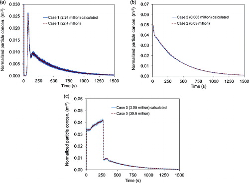
This study conducted particle number independence tests for the designed cases to determine whether or not the calculated particle numbers were sufficient for obtaining statistically meaningful results. The necessary particle numbers calculated by Equation (14)[14] were 2.24, 0.003, and 3.55 million, respectively, for Cases 1, 2, and 3. This study used the Lagrangian method with the calculated particle number to predict the particle concentration as a function of time in the target zone. To conduct the particle number independence tests, this study repeated the simulations with a particle number that was increased by a factor of 10. Figure 2 compares the normalized particle concentrations predicted from the calculated particle number with those predicted from particle number that is 10 times larger. All the particle concentrations were normalized by the total particle number injected in the room. For all three cases, the Lagrangian method with the calculated particle number provided similar results to those with a 10-times-larger particle number. Therefore, the proposed method can provide a necessary particle number with a reasonable magnitude. This method avoids the unguided process of the particle number independence test and thus significantly accelerates the entire calculation process.

FIG. 2. Particle number independence tests for (a) Case 1, (b) Case 2, and (c) Case 3.

3.3. Verification of the Methods for Reducing the Necessary Particle Number

3.3.1. Superimposition Method

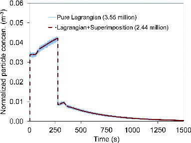
This study compared the normalized particle concentrations predicted by the combined Lagrangian and superimposition method and the pure Lagrangian method for Case 3. The necessary particle number for the pure Lagrangian method calculated by Equation (14)[14] was 3.55 million, while that for the combined method calculated by Equation (17)[17] was 2.24 million. As shown in Figure 3, the particle concentrations predicted by the combined Lagrangian and superimposition method agreed well with that predicted by the pure Lagrangian method. However, the necessary particle number in the combined method (2.24 million) was reduced by 1.6 times in comparison with that in the pure Lagrangian method (3.55 million).

FIG. 3. Comparison of normalized particle concentrations predicted by the combined Lagrangian and superimposition method and the pure Lagrangian method.

Equation (18)[18] indicates that the reduction in particle number when using the superimposition method depends on the duration of the particle source. Figure 4 shows the factor of reduction in particle number when using the superimposition method as a function of source duration (Equation (18)[18] ). The factor of reduction in particle number is positively associated with the particle source duration. For example, if the duration was 0.1 τ, the necessary particle number could be reduced only slightly when using the superimposition method. However, if the duration was increased to 5 τ, the necessary particle number could be reduced by five times when using the superimposition method. Therefore, the superimposition method can reduce the necessary particle number in the Lagrangian method when the particle source duration is relatively long.

FIG. 4. Factor of reduction in particle number as a function of particle source duration when the superimposition method is used.

3.3.2. Time-Averaging Method

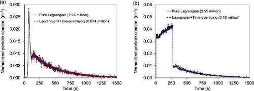
This study compared the normalized particle concentrations predicted by the combined Lagrangian and time-averaging method and the pure Lagrangian method for Cases 1 and 3. The necessary particle numbers in the pure Lagrangian method calculated by Equation (14)[14] were 2.24 million for Case 1 and 3.55 million for Case 3. In comparison, the necessary particle numbers in the combined method calculated by Equation (19)[19] for Cases 1 and 3 were 0.074 and 0.12 million, respectively. As discussed in Section 2.3.2, time-averaging can be performed over every N_target* = 30 time steps.

As shown in Figure 5, the particle concentrations predicted by the combined Lagrangian and time-averaging method agreed well with those predicted by the pure Lagrangian method for both cases. Furthermore, the necessary particle number in the combined method was reduced by 30 times as compared with that in the pure Lagrangian method. Thus, the hypothesis that the time-averaging method can reduce the necessary particle number has been verified. It should be noted that the number of time steps to be averaged depends on the level of detail required in the results. For instance, if the calculated particle concentration as a function of time with a time step size of 0.05 s is to be compared with experimental data with a measurement time interval of 0.5 s, time-averaging over more than 10 time steps is not suitable. Furthermore, the particle concentrations may vary significantly in certain time steps. To ensure that the peak particle concentrations are captured, the time-averaging method should not be used in such time steps.

FIG. 5. Comparison of normalized particle concentrations predicted by the combined Lagrangian and time-averaging method and the pure Lagrangian method for (a) Case 1 and (b) Case 3.

3.3.3. Combined Superimposition and Time-Averaging Method

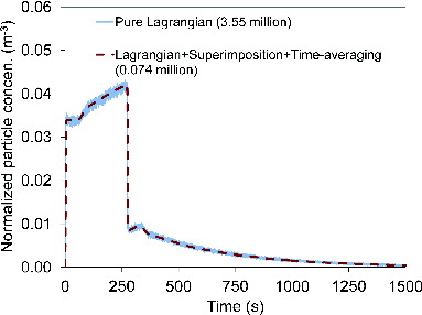
This study further compared the normalized particle concentrations predicted by the combined Lagrangian, superimposition, and time-averaging method and the pure Lagrangian method for Case 3. The calculated necessary particle number for the pure Lagrangian method was 3.55 million according to Equation (14)[14] , while that for the combined method was 0.074 million according to Equation (21)[21] . As discussed in Section 2.3.2, time-averaging can be performed over every N_target* = 30 time steps. As shown in Figure 6, the particle concentration profiles predicted by the combined Lagrangian, superimposition, and time-averaging method matched well with the profile predicted by the pure Lagrangian method. Furthermore, the necessary particle number in the combined method was reduced by 48 times as compared with that in the pure Lagrangian method. Therefore, this comparison verifies that the combined superimposition and time-averaging method can further reduce the necessary particle number in the Lagrangian method. As indicated in Equation (22)[22] , the reduction in particle number when using the combined method increases as the particle source duration becomes longer. For instance, if the duration of the particle source was 0.1 τ, the necessary particle number in the combined method would be reduced by 30 times as compared with that in the pure Lagrangian method. If the duration was increased to 5 τ, the combined Lagrangian, superimposition, and time-averaging method would reduce the necessary particle number by 150 times compared with that in the pure Lagrangian method.

FIG. 6. Comparison of normalized particle concentrations predicted by the combined Lagrangian, superimposition, and time-averaging method and the pure Lagrangian method.

3.3.4. Comparison of Computing Cost

Table 2 compares the computing time of the pure Lagrangian method and the combined methods. The computing time was estimated on a single core computer with two 3.2 GHz Intel(R) Xeon(R) processors and 12 GB of memory. For Case 1, the combined Lagrangian and time-averaging method can reduce the computing time by 30 times when compared with the pure Lagrangian method. For Case 3, the combined Lagrangian, superimposition, and time-averaging method can reduce the computing time by 40 times when compared with the pure Lagrangian method. Therefore, the proposed method can significantly save the computing resources.

TABLE 2 Comparison of computing cost

	Computing time (h)^a
Case no.	Pure Lagrangian	Lagrangian + superimposition	Lagrangian + time-averaging	Lagrangian + superimposition + time-averaging
1	48.9	N/A	1.6	N/A
3	64.8	48.9	2.2	1.6

^aThe computing time was estimated on a single core computer, with two 3.2 GHz Intel(R) Xeon(R) processors and 12 GB of memory.

3.4. Validation with Experimental Data

This study used the experimental data obtained by Zhang et al. (2009) to validate the proposed methods for predicting transient particle transport in indoor environments. This case was the same as the previous cases in all aspects except the boundary condition at the inlet. In the experiment, two optical particle counters were used to measure the transient particle concentrations at the inlet and one of the measurement locations (Points 1 and 2) simultaneously. Therefore, the experiment was conducted twice in order to obtain the results at the two locations. The inlet particle concentration profiles at Points 1 and 2 are shown in Figures 7a and b, respectively. The two profiles exhibit similar trends, but there are some differences. In general, at the inlet, there was an initial peak in particle concentration, and then the concentration decreased significantly to a stable level.

FIG. 7. Comparison of the numerical results for transient particle concentration with the corresponding experimental data: (a) Point 1 and (b) Point 2.

With the grid resolution (18,009) used in this study, the volume of the CFD cell at Points 1 and 2 was 0.0012 m³. The calculated necessary particle number in the combined Lagrangian, superimposition, and time-averaging method was 1.72 million on the basis of the proposed method. The time step size in the simulation was 0.05 s. Figure 7 compares the numerical results for transient particle concentration with the experimental data. Note that two sets of simulations were performed on the basis of the corresponding inlet particle concentration profiles. In Figure 7a, the simulation and the experiment at Point 1 both show particle concentration profiles that are similar to that at the inlet. This similarity occurred because Point 1 was close to the inlet. The fluctuations in particle concentration at this location were caused primarily by the fluctuations measured at the inlet. In Figure 7b, both the simulation and the experiment at Point 2 exhibit peak particle concentrations that are lower than that at the inlet. Moreover, the peak at Point 2 is delayed in time compared with that at the inlet. This delay indicates a weaker response to the source because of a greater distance between the source and Point 2. In comparison with the experimental data, the proposed method overestimated the particle concentrations after about 500 s. Zhang et al. (2009) compared the results predicted by an Eulerian method with experimental data. They also found that the Eulerian method overestimated the particle concentrations after about 500 s. The differences between the simulation and the experiment may be attributed to the discrepancies between the predicted airflow field and the actual one (Zhang et al. 2009). In general, the trends in transient particle concentration predicted by the combined Lagrangian, superimposition, and time-averaging method agreed reasonably well with the experimental data. Therefore, the proposed method can be used for predicting transient particle transport in indoor environments with reasonable accuracy.

4. DISCUSSION

4.1. Influence of the Coefficient α

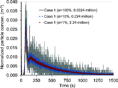
The coefficient α in Equation (14)[14] can influence the calculated necessary particle number in the Lagrangian tracking calculations. If this α is equal to 1%, the results will be statistically meaningful even when the particle concentration has decreased to 1% of the peak value. Therefore, the value of α depends on the tolerance of error. This study conducted a sensitivity analysis of α for Case 1. Figure 8 compares the normalized particle concentrations predicted by the Lagrangian method with particle numbers that were estimated using α values of 1%, 10%, and 100%. The corresponding calculated necessary particle numbers were 2.24, 0.224, and 0.0224 million, respectively. It can be seen that a smaller α provides better results, with fewer fluctuations and uncertainties. Theoretically, there is no cut-off value for α. For engineering applications, as shown in the figure, a α value of around 1% should minimize fluctuations and uncertainties in the results.

FIG. 8. Comparison of normalized particle concentrations predicted by the Lagrangian method with particle numbers that were estimated using α values of 1%, 10%, and 100%.

4.2. Equations for Other Particle Sources

In order to demonstrate the proposed methods, the analysis above used an example in which particles were emitted from the inlet. Another typical scenario is the emission of particles from a location inside the room, such as from the cough of an occupant. In this case, the boundary condition of Equation (4)[4] is:[23]

Using the approach described in Section 2.2, the equation for calculating the necessary particle number can be obtained. One finds that the equation for a particle source inside the room is identical to that for a particle source from the inlet (Equation (14)[14] ).

For some particle sources, Equation (4)[4] cannot be solved analytically with the corresponding boundary condition. One such case is that studied by Zhang et al. (2009), as described in Section 3.4. In this case, the inlet particle concentrations were time-varying, as shown in Figure 7. The study solved the equation numerically for this case by simply using Microsoft Excel. Therefore, even if the equation cannot be solved analytically, the proposed methods can be used to accelerate the Lagrangian method by numerically solving the ordinary differential equation.

4.3. Limitations of This Study

There are a number of limitations to the present work, beginning with the assumption of a steady-state airflow field, which may be a problem in some cases. For instance, transient particle transport in a building with natural ventilation is likely to have an unsteady-state airflow field. In such cases, the time-averaging method can still be used; however, the superimposition method may not be suitable. In addition, this study neglected particle deposition onto surfaces because the modeled particle size was 1 μm. However, for ultrafine or coarse particles in a room with a low air change rate, the impact of particle deposition may be considerable. Therefore, to model the transient transport of ultrafine or coarse particles, the influence of deposition should be taken into account. Although the transient airflow and particle deposition could affect the necessary particle number in the Lagrangian method, it should be noted that the proposed method is to estimate a reasonable magnitude of the necessary particle number rather than determining a precise value. Therefore, the proposed method can still be used for these scenarios.

5. CONCLUSIONS

This investigation developed a method for estimating and reducing the necessary particle number in order to accelerate the Lagrangian method for predicting transient particle transport in indoor environments. The investigation has led to the following conclusions:

1. The proposed method can estimate the necessary particle number and thus reduce the effort that is normally required for evaluating different numbers of particles in order to achieve statistically meaningful results.

2. The superimposition and time-averaging method can reduce the necessary particle number, and, as a result, the computing cost can be further reduced.

3. The combined Lagrangian, superimposition, and time-averaging method can predict transient particle transport in indoor environments with reasonable accuracy.

ACKNOWLEDGMENTS

We thank Dr. N. Zhang from McNeese State University for generously providing information about his experiment.

FUNDING

The research presented in this article was supported by the National Basic Research Program of China (the 973 Program) through Grant No. 2012CB720100.

REFERENCES

- ANSYS. (2010). Fluent 12.1 Documentation. Fluent Inc., Lebanon, NH.
- Chao, C. Y. H., and Wan, M. P. (2006). A Study of the Dispersion of Expiratory Aerosols in Unidirectional Downward and Ceiling-Return Type Airflows using a Multiphase Approach. Indoor Air, 16:296–312.
- Chao, C. Y. H., Wan, M. P., and Sze To, G. N. (2008). Transport and Removal of Expiratory Droplets in Hospital Ward Environment. Aerosol Sci. Tech., 42:377–394.
- Chen, C., and Zhao, B. (2010). Some Questions on Dispersion of Human Exhaled Droplets in Ventilation Room: Answers from Numerical Investigation. Indoor Air, 20:95–111.
- Chen, C., and Zhao, B. (2011). Review of Relationship Between Indoor and Outdoor Particles: I/O Ratio, Infiltration Factor and Penetration Factor. Atmos. Environ., 45: 275–288.
- Chen, C., Zhao, B., and Weschler, C. J. (2012). Indoor Exposure to Outdoor PM10: Assessing its Influence on the Relationship Between PM10 and Short-Term Mortality in U.S. Cities. Epidemiology, 23:870–878.
- Chen, C., Lin, C.-H., Jiang, Z., and Chen, Q. (2014). Simplified Models for Exhaled Airflow from a Cough with the Mouth Covered. Indoor Air, 24:580–591.
- Choudhury, D. (1993). Introduction to the Renormalization Group Method and Turbulence Modeling, Canonsburg, Fluent Inc. Technical Memorandum TM-107.
- Durrett, R. (2010). Probability: Theory and Examples, 4th ed. Cambridge University Press, New York.
- Gao, N. P., and Niu, J. L. (2007). Modeling Particle Dispersion and Deposition in Indoor Environments. Atmos. Environ., 41:3862–3876.
- Gupta, J. K., Lin, C.-H., and Chen, Q. (2011a). Transport of Expiratory Droplets in an Aircraft Cabin. Indoor Air, 21:3–11.
- Gupta, J. K., Lin, C.-H., and Chen, Q. (2011b). Inhalation of Expiratory Droplets in Aircraft Cabins. Indoor Air, 21: 341–350.
- Klepeis, N. E., Neilson, W. C., Ott, W. R., Robinson, J. P., Tsang, A. M., Switzer, P., Behar, J. V., Hern, S. C., and Englemann, W. H. (2001). The National Human Activity Pattern Survey (NHAPS): A Resource for Assessing Exposure to Environmental Pollutants. J. Exp. Anal. Environ. Epidemiol., 11:231–252.
- Launder, B. E., and Spalding, D. B. (1974). The Numerical Computation of Turbulent Flows. Comput. Method Appl. M., 3:269–289.
- Li, Y., Huang, X., Yu, I. T. S., Wong, T. W., and Qian, H. (2005). Role of Air Distribution in SARS Transmission During the Largest Nosocomial Outbreak in Hong Kong. Indoor Air, 15:83–95.
- Li, Y., Leung, G. M., Tang, J. W., Yang, X., Chao, C., Lin, J. H., Lu, J. W., Nielsen, P. V., Niu, J. L., Qian, H., Sleigh, A. C., Su, H. J., Sundell, J., Wong, T. W., and Yuen, P. L. (2007). Role of Ventilation in Airborne Transmission of Infectious Agents in the Built Environment – A Multidisciplinary Systematic Review. Indoor Air, 17:2–18.
- Liu, J., Wang, H., and Wen, W. (2009). Numerical Simulation on a Horizontal Airflow for Airborne Particles Control in Hospital Operating Room. Build. Environ., 44:2284–2289.
- Nicas, M., Nazaroff, W. W., and Hubbard, A. (2005). Toward Understanding the Risk of Secondary Airborne Infection: Emission of Respirable Pathogens. J. Occup. Environ. Hyg., 2:143–154.
- Occupational Safety & Health Administration (OSHA). (2014). OSHA Technical Manual (OTM). Section II: Chapter 1, Personal sampling for air contaminants. available at https://www.osha.gov/dts/osta/otm/otm_ii/pdfs/otmii_chpt1_allinone.pdf [accessed 17 October 2014].
- Ozkaynak, H., Xue, J., Spengler, J. D., Wallace, L. A., Pellizzari, E. D., and Jenkins, P. (1996). Personal Exposure to Airborne Particles and Metals: Results from the Particle TEAM Study in Riverside, California. J. Exp. Anal. Environ. Epidemiol., 6:57–78.
- Peters, A., Liu, E., Verrier, R. L., Schwartz, J., Gold, D. R., Mittleman, M., Baliff, J., Oh, J. A., Allen, G., Monahan, K., and Dockery, D. W. (2000). Air Pollution and Incidence of Cardiac Arrhythmia. Epidemiology, 11:11–17.
- Pope, C. A. III, Burnett, R. T., Thun, M. J., Calle, E. E., Krewski, D., Ito, K., and Thurston, G. D. (2002). Lung Cancer, Cardiopulmonary Mortality, and Long-Term Exposure to Fine Particulate Air Pollution. JAMA, 287:1132–1141.
- Qian, H., and Li, Y. (2010). Removal of Exhaled Particles by Ventilation and Deposition in a Multibed Airborne Infection Isolation Room. Indoor Air, 20:284–297.
- Sadrizadeh, S., Tammelin, A., Ekolind, P., and Holmberg, S. (2014). Influence of Staff Number and Internal Constellation on Surgical Site Infection in an Operating Room. Particuology, 13: 42–51.
- Spengler, J. D., Dockery, D. W., Turner, W. A., Wolfson, J. M. and Ferris, B. G. Jr. (1981). Long-Term Measurements of Respirable Sulfates and Particles Inside and Outside Homes. Atmos. Environ., 15:23–30.
- Student. (1908). The Probable Error of a Mean. Biometrika, 6:1–25.
- Wan, M. P., Chao, C. Y. H., Ng, Y. D., Sze To, G. N., and Yu, W. C. (2007). Dispersion of Expiratory Droplets in a General Hospital Ward with Ceiling Mixing Type Mechanical Ventilation System. Aerosol Sci. Tech., 41:244–258.
- Wan, M. P., Sze To, G. N., Chao, C. Y. H., Fang, L., and Melikov, A. (2009). Modeling the Fate of Expiratory Aerosols and the Associated Infection Risk in an Aircraft Cabin Environment. Aerosol Sci. Tech. 43:322–343.
- Wang, M., Lin, C.-H., and Chen, Q. (2012). Advanced Turbulence Models for Predicting Particle Transport in Enclosed Environment. Build. Environ., 47:40–49.
- Weschler, C. J. (2006). Ozone's Impact on Public Health: Contributions from Indoor Exposures to Ozone and Products of Ozone-Initiated Chemistry. Environ. Health Perspect., 114:1489–1496.
- You, R., Cui, W., Chen, C., and Zhao, B. (2013). Measuring Short-Term Emission Rate of Particles in the “Personal Cloud” with Different Clothes and Activity Intensities in a Sealed Chamber. Aerosol Air Qual. Res., 13:911–921.
- Yu, O. C., Sheppard, L., Lumley, T., Koenig, J. Q., and Shapiro, G. G. (2000). Effects of Ambient Air Pollution on Symptoms of Asthma in Seattle-Area Children Enrolled in the CAMP Study. Environ. Health Perspect., 108:1209–1214.
- Zhang, N., Zheng, Z., Eckels, S., Nadella, V. B., and Sun, X. (2009). Transient Response of Particle Distribution in a Chamber to Transient Particle Injection. Part. Part. Syst. Charact., 26:199–209.
- Zhang, R., Tu, G., and Ling, L. (2008). Study on Biological Contaminant Control Strategies Under Different Ventilation Models in Hospital Operating Room. Build. Environ., 43:793–803.
- Zhang, Z., and Chen, Q. (2006). Experimental Measurements and Numerical Simulations of Particle Transport and Distribution in Ventilated Rooms. Atmos. Environ., 40:3396–3408.
- Zhang, Z., Zhai, Z. Q., Zhang, W., and Chen, Q. (2007). Evaluation of Various Turbulence Models in Predicting Airflow and Turbulence in Enclosed Environments by CFD: Part 2 - Comparison with Experimental Data from Literature. HVAC&R Res. 13:871–886.
- Zhang, L., and Li, Y. (2012). Dispersion of Coughed Droplets in a Fully-Occupied High-Speed Rail Cabin. Build. Environ., 47:58–66.
- Zhao, B., Chen, C., and Tan, Z. (2009). Modeling of Ultrafine Particle Dispersion in Indoor Environments with an Improved Drift Flux Model. J. Aerosol Sci., 40:29–43.
- Zhu, Y., Zhao, B., Zhou, B., and Tan, Z. (2012). A Particle Resuspension Model in Ventilation Ducts. Aerosol Sci. Technol., 46:222–235.