Analysis of Particle Transport and Deposition of Micron-Sized Particles in a 90° Bend Using a Two-Fluid Eulerian–Eulerian Approach

Abstract

Two-phase flows involving dispersed particle and droplet phases are common in a variety of natural and industrial processes, such as aerosols, blood flow, emulsions, and gas-catalyst systems. For sufficiently dilute particle/aerosol phases, a simplified one-way coupling is often assumed, in which the continuous primary phase is unaffected by the presence of the dispersed secondary phase and standard CFD methods can be applied. To predict the transport and deposition of the particle phase, typically a Lagrangian particle-tracking or Eulerian one-fluid/two-phase drift-flux approach is used. Here, a full two-fluid Eulerian modeling approach is presented for coarse particles (>1 μm), in which transport equations are numerically solved for both particle-phase continuity and particle-phase momentum. Simulation results were obtained for a laminar flow regime (Re 100 and 1000) in a 90° elbow, and the effects of grid topology and resolution were investigated. Additionally, gravity effects were considered for both Re cases. Results using this full two-fluid Eulerian approach were validated against experimental data and other computational studies. One key novel contribution of this work is presentation of a simple algorithm for stabilizing the Eulerian particle-phase equation. To the authors' knowledge, this is the first study documenting a full two-fluid Eulerian approach for dilute particle phases in laminar flow on unstructured (prism/tetrahedral) meshes. The results show the potential of the two-fluid approach for providing a useful alternative to the more typical Lagrangian approach for prediction of coarse-particle transport and wall deposition.

Copyright 2015 American Association for Aerosol Research

1. INTRODUCTION

Micro- and nanoparticles have been studied widely due to unique material properties arising from their size and high surface area to volume ratio (Nalwa 2004; Best et al. 2012; Torres Galvis et al. 2012). These particles are catalogued according to size as coarse particles (>1 µm), fine particles (1 µm–100 nm), and ultrafine particles (<100 nm). In two-phase flows, the transport path of these dispersed particles does not necessarily follow the streamlines of the primary fluid. Understanding and predicting the transport and deposition of these particles is critical in developing and optimizing many medical and industrial applications such as drug delivery, blood flow, clean-coal gas turbines, and food processing (Hofmann 1996; McMurry 2000; Slater and Young 2001; Hofmann et al. 2003; Balashazy et al. 2007). Accurate prediction methods for the transport, impaction, and deposition, and fate of micro- and nanoparticles are needed, especially methods that can be applied across wide ranges of fluid-flow conditions and particle sizes.

The most common modeling approach for ultrafine particles is the one-fluid Eulerian approach, since particle- and gas-phase velocities are nearly identical, and transport of the particle phase is strongly governed by molecular diffusion (Brownian motion). For coarse particles, the Lagrangian particle-tracking approach is the most common for low Reynolds number flows, since due to inertial effects particle velocities can differ substantially from the surrounding gas phase, and molecular diffusion is negligible (Shi et al. 2007). For high Reynolds number flows, turbulent mixing is typically modeled as a diffusion process, and some studies have adopted a two-fluid Eulerian approach (Mohanarangam et al. 2008; Dehbi 2011). Far less common is the use of a two-fluid Eulerian approach for coarse particles in laminar flow. First, the diffusion term is small relative to turbulent flow, which tends to reduce the stability of the algorithm. Second, the presence of numerical dissipation in the particle-phase convective terms may lead to non-physical mixing or smearing of the particle phase and inaccurate results. Both of these effects are expected to be exacerbated on unstructured meshes. To the authors' knowledge, no studies are available in the literature for dilute (one-way coupled), low-Reynolds number gas-course particle flows, using a full two-fluid Eulerian approach on unstructured grids.

In some cases, it is advantageous to consider the use of a two-fluid Eulerian approach for coarse particles. To cite a specific example, recent studies of lung airflow have adopted simplified airway geometries in which only a small fraction of the branches are retained at each successive generation. The general methodology is outlined in Walters and Luke (2010, 2011) and an example using a patient-specific airway geometry may be found in Walters et al. (2011). Because this method leads to a large number of non-terminal flow outlets, approximately 50% of particles will be lost at each generation using a Lagrangian method. In order to retain ˜10,000 particles in each terminal generation, approximately 100 billion particles would need to be instilled at the oronasal opening. In order to reduce the associated computational expense, it is desired to adopt an Eulerian method that asymptotically approaches the one-fluid model for ultrafine particles and provides reasonable results for larger particles. This article seeks to propose and validate such a method on a canonical test case.

As model validation is only as good as the experimental data, it is important to document and match the experiment details and to understand the reasons for reported problems identified in experimental and computational datasets. For example, the models by Pui et al. (1987) and McFarland et al. (1997) were found to be inaccurate when applied to large droplets and high radial velocities experienced in industrial bends. As a result, particle deposition models for industrial ducts (Peters and Leith 2004a, 2004c) and 90° bends in exhaust ventilation systems (Peters and Leith 2004b) were proposed to better match experimental data. Therefore, accuracy in detailing geometries, experimental parameters, and simulation components become critical as CFD models are implemented—even on simple grids—to predict particle transport and deposition.

Several previous studies have investigated both Eulerian and Lagrangian methods for simulation of dispersed particle phases. Pilou and coworkers (Pilou et al. 2011) investigated particle deposition in a 90° bend using an Eulerian approach with a modified convective diffusion equation based on a near-wall velocity correction effect for the drift-flux equation (Oldham et al. 2000; Longest and Oldham 2008). The same authors simulated physiologically realistic bifurcations representative of generations G3–G4 of the human lung, and results were used to predict particle deposition (Pilou et al. 2013). The 90° bend results were compared with previous modeling and experimental data published by Pui et al. (1987). In fact, the experimental work of Pui and coworkers has been extensively compared with CFD results using Eulerian or Lagrangian simulations for particle-tracking. For example, Breuer et al. (2006) used a Lagrangian particle-tracking and deposition approach for laminar and turbulent flows; however, the number of particles was found to affect deposition results even at high particle loadings. Another study of the same test case used a coupled Eulerian method to solve for particle deposition (Armand et al. 1998), but kinematic viscosity and particle acceleration due to gravity were both neglected. Data from the experimental work performed by Pui et al. (1987) were compared with the analytical work of Cheng and Wang (1981) but only fitted for large Dean (De) numbers. Later it was determined that the inlet profile and De number affect the deposition efficiency in the 90° elbow (Tsai and Pui 1990), and that incompatibilities at low De numbers were a result of the inefficacy of capturing a boundary layer and a core region at this particular low De number. All of the Eulerian methods discussed above, with the exception of the work of Armand et al. (1998) and Mohanarangam et al. (2008), were predicted using a one-fluid Eulerian approach, where particle velocity is assumed to be equal to the air velocity or is obtained using a drift-flux approximation. Furthermore, the work of Mohanarangam investigated only turbulent flow simulations, which improve stability through the use of a turbulent viscosity term, and the simulations of Armand were only performed on structured grids. In this work, the experimental data of Pui et al. (1987) are used to evaluate the results obtained from a full two-fluid Eulerian–Eulerian methodology for laminar flow on unstructured meshes. A new discretization method for the convective term is introduced to ensure stability of the simulations.

Modifications to typical Eulerian methodologies for particle transport and deposition have been recently reported in the literature and are a current focus of CFD simulation research. Longest and Oldham (2008) developed a new method with velocity corrections where the drift flux Eulerian equations were coupled with a Lagrangian-based boundary condition approach near the wall on a double bifurcation model. This method was also implemented by Xi and Longest (2008a) in a tracheobronchial representative grid and compared with experimental data in a nasal cavity replica cast for various particle diameters ranging from 1 to 1000 nm. The drift-flux equation accounts for particle inertia and diffusion when determining the total particle deposition. This hybrid combination of Eulerian and Lagrangian methods was also used by Pilou et al. (2011) in the 90° bend described earlier. An important finding is that the computational time was significantly reduced using the new implementation of the drift-flux velocity correction method as compared with typical Lagrangian simulations. Another advantage of this method was improved particle deposition percentage prediction, as compared with experimental results and the generalized chemical species (CS) Eulerian equations (Longest and Oldham 2008). These results suggest that improving Eulerian two-fluid methods may allow for significant improvements in overall simulation capability for these flows.

Lagrangian particle-tracking methods and improved turbulence models have also been investigated and research in these areas is ongoing. For example, studies of a Lagrangian particle-tracking model with a particle-wall collision model used to predict flow movement and deposition of particles (1, 3, 5, 9, and 16 μm) in a 90° ventilation duct have been previously conducted (Sun et al. 2011). In a different study, the turbulent renormalization group (RNG) k-ϵ model was used along with Lagrangian particle-tracking to predict turbulent air and particle flow (Jiang et al. 2011). The particle penetration rates were validated in a test duct at six different Stokes numbers. Reynolds–Averaged Navier–Stokes (RANS) Lagrangian methods for dust (ranging from 10 to 200 µm) deposition in square-shaped duct bends with different injection points were also recently developed with the effects of drag, lift force, gravity, inertia force, and turbulent diffusion considered (Gao and Li 2012). A notable finding was that gravity and inertia force increased the deposition rate as relaxation time increased. Turbulent particulate-laden flows in curved pipes using a RANS approach in ANSYS Fluent were studied with different bend angles, bend curvature ratios, and various Reynolds numbers (Zhang et al. 2012). An Enhanced Wall Treatment (EWT) combined with the linear pressure-strain Reynolds Stress Model (RSM) method was proposed for modeling particle deposition in flows with curved streamlines. Complex grids, such as the human lung, require a large number of particles to estimate particle deposition values using Lagrangian methods. This limitation combined with the inherent issue of a large number of particles to be considered with one-fluid velocity approach opens the need for improved methods for Eulerian two-fluid models and deposition methodologies. Therefore, we propose that improvements in modeling techniques are needed regardless of the current state of Lagrangian, one-fluid Eulerian, and drift-flux modeling approaches for coarse particles.

In this work, a two-fluid Eulerian method that independently solves particle-phase continuity and momentum equations is applied to a 90° bend geometry, and validated with the experimental work of Pui et al. (1987). The main objectives of this work are to: (1) develop a full two-fluid Eulerian approach to simulate particle flow and deposition that is both stable and of sufficiently high resolution so that mesh independent results can be obtained on unstructured grids; (2) analyze two laminar flow cases (Re = 100 and Re = 1000) using the approach, comparing gravity effects and grid dependence; (3) compare the particle Eulerian results with published experimental and simulation data; and (4) analyze the Eulerian–Eulerian two-fluid approach in a hybrid mesh (rectangular and tetrahedral cells) to account for the near-wall interactions and deposition of particles. Future work should evaluate other conditions such as turbulence, thermophoretic forces, non-spherical and non-homogeneous particles, and other critical parameters that could affect particle deposition.

2. METHODS

Simulations were carried out using the commercial software Ansys FLUENT version 14 and grids were constructed using Ansys Gambit version 2.4. The primary (air) phase was computed using built-in algorithms in FLUENT. The secondary (particle) phase continuity and x-, y-, and z-momentum equations were implemented for User-Defined Scalar variables particle volume fraction, and particle-phase x-, y-, and z-velocity, respectively. All terms in the equations were implemented using User-Defined Function (UDF) subroutines. The overall methodology is described in the following sections. First, the governing transport equations and boundary conditions for the airflow velocity are described. Next, the two-phase Eulerian model used in this work is discussed. Finally, a summary of the simulation details and the two different computational elbow grids with different levels of mesh refinement are presented.

2.1. Fluid Phase: Airflow Velocity

For the primary (air) phase, steady state, incompressible, laminar flow was considered for solution of the Navier–Stokes equations. The assumption of laminar flow was considered valid based on the recommendation by Pilou et al. (2011) and the experimentally measured Reynolds numbers (Pui et al. 1987). The steady-state governing equations for conservation of mass and momentum in the primary phase are shown below:[1] [2] where is the air-phase velocity vector, is the pressure, is the air-phase density, and is the kinematic air viscosity.

The equations were solved using a finite-volume approach. The SIMPLE pressure correction scheme (Patankar and Spalding 1972) was used for pressure-velocity coupling, with momentum-weighted interpolation of face mass fluxes (Rhie and Chow 1983), to avoid checkerboarding due to the collocated mesh arrangement. The pressure staggering option (PRESTO!) scheme (Ansys, Inc. 2009), which uses a discrete continuity balance at the cell face for pressure computation, was used to discretize the pressure term. A second-order upwind scheme with monotonic slope limiting (Barth and Jespersen 1989) was used to discretize the convective terms. A second-order central difference scheme was used to discretize the diffusion terms. All gradients were computed to second-order accuracy using a node-based Green-Gauss method.

A prescribed velocity profile was used as the inlet boundary condition. The airflow velocity was initially solved using a parabolic velocity profile as suggested by Tsai and Pui (1990). The outlet was defined as a constant pressure boundary condition. The walls were defined as impermeable and no-slip with respect to the air phase.

2.2. Particle-Phase Analysis: Two-Fluid Eulerian Approach

A full two-fluid approach was adopted for prediction of the particle-phase transport. Governing differential equations were solved for particle volume fraction and momentum, in contrast to the drift-flux method in which an algebraic approximation is solved for particle-phase velocity. The governing equations solved for the two-phase Eulerian model were obtained based on the assumptions of a dilute phase (one-way coupling), very high particle-to-air density ratio, and only gravity and drag forces acting on individual particles. The resulting simplified equations in their steady-state form are:[3] [4] where is the particle-phase volume fraction, is the particle-phase velocity, and is the volume of the particle. Note that particle-phase pressure and viscous stresses are assumed negligible. Particle drag force () was calculated based on the assumption of low particle Reynolds number and is represented by[5] where is the viscosity of the air, and Re_p is the particle-phase Reynolds number, defined as[6] where d_p is the diameter of the particle and C_D is the drag coefficient, which is obtained from the model of Morsi and Alexander (1972) based on smooth, spherical particles, and computed as[7] As stated above, the particle-phase equations were obtained considering only gravity and drag forces. Other forces such as thermophoresis, lift, and Brownian motion (negligible diffusion coefficient) could be included for cases in which they are non-negligible.

A uniform particle concentration was set as the boundary condition at the 90° elbow inlet. Since the particle phase is assumed to be dilute, with one-way coupling between the primary and secondary flow, and because all terms in the governing equations scale linearly with , the volume fraction was arbitrarily set to one at the inlet. Simple convection boundary conditions were applied at the outlet, and no reverse flow regions were present for the simulations performed here.

Previous studies have demonstrated that treatment of the wall boundary conditions for the particle phase is a critical component of the two-fluid Eulerian approach, and modification of the wall boundary conditions was carefully addressed in the current study. Inertial deposition is represented as a particle-phase convective flux out of the domain. For the finite-volume formulation adopted here, specification of the convective flux requires estimation of the particle-phase volume fraction and velocity component at the wall. The simple approach adopted in the current study assumes a first-order zero-gradient approximation for the velocity components:[8] where n_j is the wall unit normal vector pointing out of the domain. In practice, this assumes that the wall velocity is equal to the velocity in the first near-wall computational cell. The volume fraction at the wall is computed based on the direction of particle-phase velocity:[9] [10] When the particle-phase velocity is out of the domain, a first-order zero-gradient approximation is used, and the volume fraction at the wall is equal to the volume fraction in the first near-wall cell. When the particle-phase velocity is not out of the domain, the wall volume fraction is assumed to be zero.

More advanced wall boundary condition methods were implemented and tested, including second-order linear projection of velocity and volume fraction values to the wall from the first-layer cells, and the Lagrangian-based model of Longest and Oldham (2008). Interestingly, neither method was found to make a significant change in the results. Example results for total deposition fraction comparing the Lagrangian-based model and the first-order model are shown in Table S1 (see Section S1 of the online supplemental information [SI]). The maximum difference was found to be 1.1%, and the average difference was <1%. The relative insensitivity to boundary condition method is believed to be due to the refinement level of the near-wall meshes used in this study relative to the coarse particle sizes investigated. The coarsest near wall mesh used a first-cell size of 7 μm, with a corresponding distance from the wall to the first cell centroid of 3.5 μm. By comparison, the smallest particle diameter investigated in this study was 5.39 μm. Application of the methodology presented here to fine particles (diameter <1 μm) would likely necessitate the use of the more advanced wall boundary condition techniques to ensure accurate results.

2.3. Discretization Methods: Finite Volume Scheme

Two key potential numerical difficulties arise when using Eulerian two-fluid finite-volume methods for solution of coarse particle phases. The first is numerical error, which manifests as diffusion for upwind-biased numerical methods. Physical diffusion mechanisms are negligible in the cases examined here, since both molecular (Brownian motion) and turbulent diffusion are assumed zero. As a consequence, any numerical diffusion may have a significant impact and lead to error in the results. The effect of numerical error can be quantified and judged to be sufficiently small using a mesh resolution study, and this is described in detail below.

The second difficulty concerns the stability of the particle-phase equations. In particular, the convective flux term in the volume fraction equation is not divergence free for the case of a uniform volume fraction field, i.e.,[11] in general. In the finite-volume method, the equations are applied in integral form over discrete computational control volumes (cells). The consequence of Equation (11)[11] can lead to non-smooth and even unstable solutions. This problem was found to be exacerbated on unstructured grids, and in the absence of any diffusion terms to stabilize or smooth the numerical solution. In fact, preliminary evaluations using the built-in two-fluid Eulerian solver available in Ansys FLUENT were not consistent and led to unstable or non-converged solutions for some particle sizes. One of the key contributions of this work is the development of an upwind-biased scheme for the convective terms in the particle-phase volume fraction equation that allows stable and accurate solutions on unstructured meshes with negligible physical diffusion.

The convection terms in integral form for the finite-volume method are constructed over generalized polyhedral cells with polygonal faces defining the interfaces between neighboring cells. Integration of the convective term and application of Green's theorem results in an expression for each cell of the form[12] where the summation on the right-hand side is over each face bounding cell C, with a total number of faces . The quantities , , and represent the numerical approximations to the average face value of the volume fraction, the convective velocity at the face, and the face area vector, respectively. The dot product represents a numerical approximation to the volumetric flow rate across each face (positive outward). The analogous expression for the convective term in the particle-phase momentum equation is[13] where an additional vector-valued variable represents the numerical approximation to the face-averaged particle-phase velocity. Note that we here adopt the practice of different approximation methods for the convective and convected face velocities (, ), which is common for upwind-biased schemes applied to incompressible flows.

The face-averaged quantities in each of the above are approximated using nominally second-order reconstruction schemes. The convective velocity is approximated using a general second-order method that recovers a centered average on uniform structured grids:[14a] [14b] [14c] where the subscripts and denote the (arbitrary) left and right side cell neighbors for a given face , respectively. The vector is the vector connecting the left-side cell centroid with the face centroid, and is the vector connecting the left-side and right-side cell centroids.

The convected velocity is obtained using a second-order upwind linear reconstruction approach with slope limiting to prevent non-physical oscillations in regions with steep variable gradients (Barth and Jespersen 1989):[15] where and are the velocity vector and velocity gradient stored in the upstream neighbor cell, and is the vector connecting the upstream cell centroid and face centroid. A cell is considered the upstream neighbor if the convective velocity vector at the face points out of the cell, i.e., for the upstream cell of a particular face , the quantity is greater than zero. For the current study the gradient is computed using a cell-based unweighted least-squares method that is linearity preserving, and each component of the gradient is limited such that the projected face values lie within bounds determined by the cell values in the vicinity of the upstream cell. The reader is referred to Barth and Jespersen (1989) for more details of the projection and limiting procedure. The procedure outlined here for the particle-phase momentum equations is identical to that used in Ansys FLUENT for the air phase and is a commonly used method for discretization of the convective term for incompressible flow simulations.

For the particle-phase volume fraction equation, a modified approach to the above was implemented to improve stability. The variable was first projected to each face from both the upstream and downstream cell neighbors, using the least-squares approximation to the gradient and slope limiting as described above:[16] [17] where and are the face values projected from the upstream and downstream cell neighbors, respectively. It was found that simple upwinding () led to an unstable solution and, in cases where convergence could be obtained, noisy results with apparently random, high wavenumber error components. To mitigate this, a weighted combination of the upstream and downstream projected values was used, for which[18]

The face integration scheme represented by Equation (18)[16] stabilizes the computation by introducing a counter (upstream) flux if the volume fraction in the downwind cell () becomes excessively large. The scheme described above is formally second-order accurate since both upwind and downwind states are computed by linear reconstruction, in regions where the slope limiter (Barth and Jepsersen 1989) is not activated, i.e., in smooth regions of the variable field. To further enhance stability, the volume fraction face values projected from the cell neighbors are limited such that they lie within the bounds:[19] [20] Finally, the face value obtained from Equation (18)[16] is limited so that no non-physical negative values are used:[21]

2.4. Grid Style, Topology, and Refinement Studies

A 90° bend grid was constructed based on the description provided by Pilou et al. (2011), matching the experimental study of Pui et al. (1987). Two different grids were generated for two different laminar flow test cases using Ansys Gambit v. 2.4. The two test cases corresponded to Re = 100 (De = 38) and Re = 1000 (De = 419), respectively, where Reynolds number is based on mean air velocity and tube diameter. Figures 1a and b show the computational domain for the Re = 100 and Re = 1000 test cases. All grids were constructed using a hybrid methodology that included a combination of tetrahedral and prismatic cells. Tetrahedral cells were used in the core of the tube, and prismatic cells were used in a near wall layer in order to better resolve the boundary layer and the particle-phase dynamics very close to the wall. Figures 1c and d show an example of the hybrid mesh topology on the Re = 1000 case, including the hybrid prism/tet distribution for a cross-section at the flow outlet and the triangular surface mesh at the wall.

FIG. 1. Geometry and grid for the 90° bend for two different laminar flow cases: (a) Re = 100, and (b) Re = 1000. Mesh topologies for the Re = 1000 grid: (c) hybrid mesh shown for a cross-section at the flow outlet, and (d) a triangular surface mesh used at the wall.

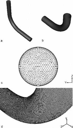
In order to investigate the effect of mesh resolution level on the results, a mesh refinement study was performed for each Reynolds number for the largest and smallest particle sizes. The mesh was successively refined until results showed no appreciable change in the results in terms of overall deposition percentage and qualitative examination of deposition pattern. The resulting two-grid independent meshes were then used to run the simulations for both Reynolds number and for all particle diameters. Results were also obtained for all cases on the coarsest (baseline) meshes. For the Re = 100 case, the coarse mesh consisted of 150 K cells and the refined (grid independent) mesh consisted of 1 M cells. For the Re = 1000 case, the coarse mesh consisted of 500 K cells and the refined mesh consisted of 3.3 M cells. The results section below includes a discussion on the effect of mesh refinement for all of the simulations performed.

2.5. Simulation Details

The two different Reynolds numbers investigated (Re = 100 and Re = 1000) correspond to two of the test cases performed by Pui et al. (1987). The two cases also had different geometries for the 90° elbow. The Re = 100 case had a ratio of elbow curvature radius to tube radius (R/r) of 7. The Re = 1000 case had R/r = 5.7. The corresponding De number was 419 and 38 for the Re = 100 and 1000 cases, respectively. Different particle sizes were analyzed for each Reynolds number of study and later compared with experimental results-based Stokes number as previous studies suggested. Details comparing particle sizes and Stokes number can be found in Table S2 (see the SI). Particle density was specified to be 895 kg/m³ as described by Pui et al. (1987). For each separate simulation, particles were also considered homogeneous in size with spherical shape.

3. RESULTS AND DISCUSSION

3.1. Fluid Phase: Air Velocity Distribution

Eulerian simulations were performed first to determine the air velocity distributions for the elbow geometry. At the entrance, a parabolic velocity profile boundary condition was imposed using a maximum velocity of 3.37 m/s for Re = 100 and 7.72 m/s for Re = 1000, based on the assumption of fully developed pipe flow in the experimental setup (Pui et al. 1987). The center-plane velocity magnitude contours for the airflow are shown in Figure 2a for the Re = 100 case. At this low Reynolds number, the streamwise velocity is affected only slightly by the elbow bend curvature, maintaining a relatively full profile throughout the bend. The velocity contours for the Re = 1000 case are shown in Figure 2b. At this higher Reynolds number, the 90° bend has a significant influence on the velocity profile showing relatively strong asymmetry in the bend region and at the exit of the elbow geometry. These results agree well with prior studies of flow in elbow geometries (Zhang et al. 2004).

FIG. 2. Airflow velocity profiles for the 90° bend for Re numbers (a) 100 (De = 38), and (b) 1000 (De = 419).

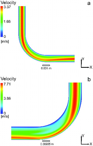
In order to validate the air velocity profiles obtained with our method, results were compared with those previously reported in the literature and this is presented in the Section S2 of the SI. As shown in Figure S1 (see the SI), axial airflow velocity profiles match very well with the results reported by Tsai and Pui (1990) and Pilou et al. (2011). The airflow velocities overlay with the prior results for both symmetry planes (z = 0 and x = 0). Using this method, airflow velocity asymmetry was again observed for Re = 1000 (z = 0) due to the elbow curvature and confirms the results shown in Figure 2. Symmetric deformations were also observed across the perpendicular symmetry plane (x = 0), as expected (more details in Section S2 in the SI).

Secondary flow (normal to the streamwise direction) velocity vectors are shown superimposed on axial velocity magnitude contours for both cases in Figure S2. The flow is shown in-plane at a 45° location and at the exit of the 90° bend section; for both Re cases, vector lengths are normalized by the inlet velocity. The development of secondary flow vortices is apparent in both cases, including the formation of symmetric counter-rotating vortices at different locations (Section S3). In brief, for Re = 100, the vortex centers are slightly displaced from the center to the outer wall, while for Re = 1000, the vortex centers show a significant shift towards the inner wall. It is also apparent that the relative strength of the secondary flow is greater for the higher Re case, as expected and comparable with the results of Pilou et al. (2011).

3.2. Particle Transport and Deposition Studies

After confirming an appropriate Eulerian solution for the airflow velocity profile, particle-phase and transport analysis with the proposed Eulerian technique are discussed for the same two laminar flow cases (Re = 100 and Re = 1000). First, a discussion on the largest Reynolds number laminar flow case (Re = 1000, De = 419) is presented. Next, particle deposition results for the second laminar flow case (Re = 100, De = 38) are summarized and contrasted with previous studies. Then, a grid refinement study discussion is presented. Lastly, the effects of gravitational forces on total particle deposition percentage are then analyzed for both cases. More details discussing fluid properties, case descriptions, and Re, Stokes, and De number calculations are found in Table S3 and further discussed in Section S4.

3.2.1. Case I: Eulerian–Eulerian Particle-Phase Transport and Cumulative Deposition Results for Re = 1000, De = 419

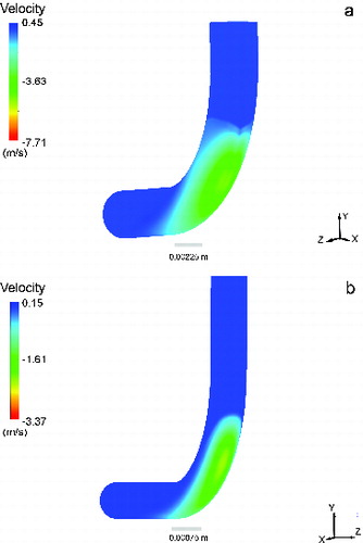
Available Lagrangian particle-tracking techniques require high computational times and large numbers of particles to be injected at the inlet of a particular grid to reach an accurate particle deposition percentage value, as discussed by Xi and Longest (2008a,b). As explained in Section 2.2, a full two-fluid Eulerian approach is adopted here to predict particle-phase velocity, which is expected to differ from the airflow velocity due to the particle inertia effects, and which includes a non-zero wall normal velocity component due to the elbow curvature. To analyze this effect, the y-component of the particle velocity at the elbow wall is shown in Figure 3 for both cases. As observed for the Re = 1000 case (Figure 3a) the impaction of particles at the curvature is very significant, allowing the particles to flow out of the fluid domain and representing impact and deposition at the elbow wall. Particle deposition is very sensitive at the near-wall region zone due to the relatively complex particle concentration field; therefore, a quantitative comparison has been made and contrasted with other simulation methods available in literature.

FIG. 3. Y-component of the particle velocity for Dp = 11.5 microns: (a) Re = 1000; (b) Re = 100.

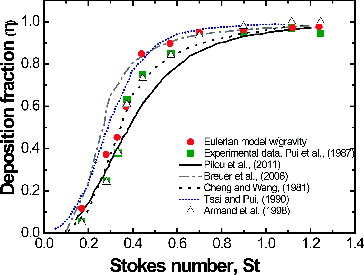
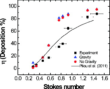
Quantitative results for total particle deposition percentage using the highest level of mesh refinement, including gravity effects, are shown in Figure 4, and these data are in close agreement with the experimental results (Pilou et al. 2011) and other simulation approaches available in literature. For example, simulation data from the most recent simulation results on this 90° bend (Pilou et al. 2011) showed a trend towards underestimation of the particle deposition as Stokes number increased. For this case, the results obtained in this study showed better agreement with experimental data for the cumulative particle deposition percentage at high Stokes number (Pui et al. 1987). Moreover, as shown in Figure 4, these results are also in agreement with previous studies, including the analytical work of Cheng and Wang (1981), Tsai and Pui (1990), Breuer et al. (2006), and the two-phase flow analysis of Armand et al. (1998). At high Stokes numbers, cumulative particle deposition is in agreement with experimental data, the simulations of Breuer et al. (2006), and the theoretical framework of Tsai and Pui (1990). Interestingly, at low Stokes numbers the two-fluid Eulerian simulation results are closer to the experimental results as compared to computational studies previously discussed. Thus, some level of improvement is apparently shown for the cumulative particle deposition fractions in a 90° bend as compared with previous computational methods available in literature.

FIG. 4. Comparison of deposition percentage for Eulerian and Lagrangian simulations and experimental data for 0.1–1.3 Stokes numbers (Dp 5.69–15.8 microns) at Re = 1000.

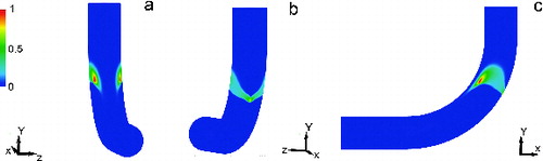
To further understand particle deposition effects, particle-wall deposition patterns are shown for 9.15 micron-sized particles for the Re = 1000 case in Figure 5. Locations with high particle deposition rates were observed just downstream of the initial curvature of the 90° bend, where greater impaction of particles in the y-direction occurs, as previously discussed (Figure 3), and in closer proximity to the elbow walls (Figures 5a and c). Interestingly, a high concentration of particles was also observed in near proximity to the inner wall, where a lower air velocity magnitude exists, and the presence of secondary flow vortices seems to affect particle deposition patterns on the inner walls (Figure 5b). This particle deposition behavior was observed for all particle sizes larger than 9.15 microns at Re = 1000, suggesting particle deposition at the entrance of the elbow curvature is due to particle impaction and large inertial effects.

FIG. 5. Particle deposition patterns (a–c) at Re = 1000 for 9.15 micron diameter particles. Contours show normalized deposition rate.

3.2.2. Case II: Eulerian–Eulerian Particle-Phase Transport and Cumulative Deposition Results for Re = 100, De = 38

To further validate the two-fluid Eulerian method of this study, the agreement between the Eulerian particle transport simulations and experimental data was also investigated using a second 90° elbow case. This second laminar flow case was run at Re = 100 (De = 38). For this case, results were compared to experimental data by Pui et al. (1987), as well as the recent low Re (De) number study performed by Pilou et al. (2011). Cumulative particle deposition percentages for the Eulerian simulations are presented in Figure 6 along with experimental data and the simulations of Pilou et al. (2011). Results suggest that the Eulerian simulation predictions compared reasonably well with experimental values for small particle sizes (˜ 5 micron). However, as the particle size increased (larger Stokes numbers), the total particle deposition percentages were significantly over-predicted in comparison to the experimental data.

FIG. 6. Cumulative particle deposition (%) in the 90° elbow for particle diameters ranging from 5.39 to 12.20 microns at Re = 100 from the two-fluid Eulerian method prediction at the highest level of refinement, experimental data (Pui et al. 1987), and prior simulation results (Pilou et al. 2011).

In contrast to the current study, previous simulations by Pilou et al. (2011) under-predicted the experimental data for deposition fraction at high Stokes numbers, as shown in Figure 6. The current simulations also show a substantial increase in deposition from Stokes number 0.6 to 0.8, which was not seen by Pilou et al. (2011). Key differences between the two studies include the mesh topology, the use of a drift-flux model in the previous study, and the inclusion of gravitational effects in the present results. The effect of gravity is also discussed below in more detail, but was found to be small for both studies, relative to the differences between studies. It is likely that one major contributor to the difference in results from the present study and Pilou et al. (2011) is due to the use of a full transport model rather than a drift-flux model for the particle-phase velocity. A representative diameter for the large particles investigated is 10 μm, with a corresponding particle relaxation time of[22] A characteristic convection time scale can be computed based on the mean velocity and the tube diameter as[23] The ratio is therefore small but on the order of unity, and it is expected that particle-phase history effects may be important. Note that as the particle size decreases, or the flow Reynolds number increases, the ratio becomes smaller and the drift-flux model is expected to more closely match results for particle-phase velocity obtained from the full transport equations. It should also be noted that the differences in mesh topology and resolution, and differences in the numerical methods, may contribute differences between the current and previous studies.

3.2.3. Grid Refinement Studies

Two different levels of grid refinement were compared for all simulations in order to determine the degree to which mesh resolution level impacted predicted particle deposition efficiency. A coarse grid consisting of 500 K cells and a refined grid of 3 M cells were utilized for this refinement study at the specified Re = 1000 (De = 419) laminar flow conditions using the two-fluid Eulerian approach. In comparing results of the two refinement levels (Figure 7a), similar results were obtained and the total particle deposition efficiency was not impacted by reducing the grid size. Moreover, the effect of gravity was also examined for each level of refinement, and no significant differences were obtained for each Stokes number (Figure 7a) at the highest level of refinement. Results of the two-fluid Eulerian modeling approach presented in this study match experimental data, validate the theoretical framework, and demonstrate that there are negligible grid refinement effects when large Re and De numbers are used (Re = 1000, De = 419).

FIG. 7. (a) No significant difference in deposition percentage was observed at Re = 1000 due to grid refinement for Stokes numbers from 0.1 to 1.3 (corresponding to 5.69–15.8 micron particle diameters). (b) At Re = 100, the effects of gravity and two grid refinement levels, “coarse” (150 K cells) and “refined” (1 M cells), were examined as a function of Stokes number. Experimental data from Pui et al. (1987).

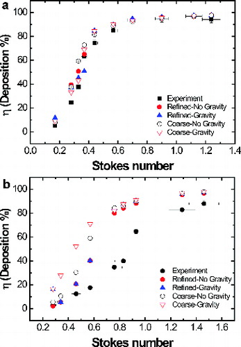
Lastly, a grid refinement study was conducted to determine any effect of grid resolution on the obtained results at low Re. For this particular case (Re = 100, De = 38) two levels of refinement were also analyzed, corresponding to a coarse grid (150 K cells) and a refined grid (1 M cells). Both grids produced very similar results for the deposition percentage for Stokes numbers larger than 0.8. However, for Stokes numbers below 0.8, there was a significant effect in predicted deposition percentage, as depicted in Figure 7b. Overprediction of particle deposition percentage occurred on a coarse grid as compared with the refined grid. Thus, grid refinement levels are significant, in particular, for low Stokes/Re number. Additionally, at the lowest grid refinement level, gravity effects had a noticeable effect on particle deposition values, whereas no difference was observed for the highest level of refinement; but, future efforts will emphasize grid convergence studies at low Stokes number, in particular for cases for which unstructured meshes are utilized. For the algorithm utilized in this work, at low Reynolds and De numbers (Re = 100, De = 38), cumulative particle deposition predictions reach grid-independent results on much coarser grids for large Stokes numbers where inertial forces are dominant but require higher mesh resolution levels to reach grid independence for small Stokes and particle Reynolds numbers.

3.2.4. Gravity Effects on Cumulative Particle Deposition

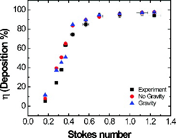
To analyze the effect of gravity in the described Eulerian modeling, a comparison was made between the experimental results (Pui et al. 1987) and simulations run both with and without gravity for the Re = 100 case (Figure 6) and the Re = 1000 case (Figure 8). Interestingly, for the latter case (Re = 1000), no significant differences were observed for particle deposition at Stokes numbers larger than 0.6 regardless of whether gravity was considered or not. In particular, at Re = 1000 and at high Stokes number, higher inertial effects are present and particle deposition is unaffected by gravity agreeing with the results shown by Pilou et al. (2011). For Stokes numbers less than 0.6, small differences in particle deposition percentage were observed due to gravity effects when comparing our results with experimental results and no gravity conditions (Figure 8) (Pui et al. 1987). As discussed below, the degree to which gravity influenced the simulations is significantly influenced by mesh refinement level, and it is likely that a more highly refined mesh would have resulted in less of an apparent influence of gravity. The small differences observed may therefore be a consequence of an under-resolved particle-phase flowfield. It should also be noted that Pilou et al. (2011) concluded that gravitational effects are not significant for the high Re/De case. Observation of Figures 6 and 8 indicates that, in the current study, gravitational effects are also found to be less significant for the higher Re/De than the lower Re/De case.

FIG. 8. Eulerian–Eulerian simulation data (with and without gravity) for Re = 1000 at refined mesh levels compared with experimental results obtained by Pui et al. (1987).

For Case II (Re = 100), despite the over-predicted results against experimental data (Figure 6), gravity seems to slightly affect cumulative deposition percentage predicted using the Eulerian–Eulerian model developed in this study. For mid-range Stokes numbers (0.7 < St < 1.0), gravity tends to increase deposition rate a small amount, though the difference due to gravity is quite small relative to the difference between experimental and computational results. As for the Re = 1000 case, it is possible that the differences are in fact due to a slight under-resolution of the flowfield, and that an increase in mesh refinement would reduce the difference even further. For the high Stokes number cases (St >1.3), almost all of the particles are deposited due to inertial impaction and gravity and therefore has little effect on results. Note that Pilou (2012) showed an effect of gravity in the Re = 100 case only for the largest particle sizes, i.e., St >1.3, and, interestingly, showed that gravity in the y-direction reduced rather than increased the deposition fraction. As discussed in the previous section, it is expected that the high Stokes number, low Re regime is precisely the one for which differences between a drift-flux method and the current simulation method will be the largest. It is therefore possible that the differences in behavior are due to fundamental differences in the computational methods. At present, the authors are not aware of any additional studies that have investigated the effect of gravity for the Re = 100 case; likewise, experimental data with no gravitational effects are not available. For purposes of validation, the results of Pilou (2012) form the best available basis for comparison. We stress once more, however, that the effects of gravity are found to be relatively small for both studies, despite the fact that the details of those effects differ.

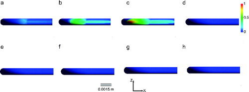
To further understand the effects of gravity at Re = 100, a qualitative study was also performed. Figure 9 shows contours of deposition rates on the bottom wall (the outer wall region downstream of the elbow bend). Results shown include the effect of gravity and were obtained using the highest level of grid refinement (1 M cells) performed in this study. For relatively small particle sizes (Figures 7a–c), deposition primarily occurs downstream of the elbow bend on the bottom wall. For larger particle sizes, results show that deposition patterns occurred primarily close to the curvature/bend on the elbow bottom walls, which were affected by particle size. In particular, this effect is clearly observed for small Stokes numbers (small particle diameter; Figures 9a–c). Additionally, particle size (Stokes number) has an effect on impaction and particle deposition fraction around the elbow walls (Pilou 2012). Larger particles with higher inertia impacted faster just downstream of the initial curvature of the 90° elbow; however, smaller particles impacted after the bend curvature and at the outer elbow wall at smaller levels (Figures 9a–c). As the Stokes number increases (larger particles), deposition occurs close to the curvature entrance, on the outer wall, where there is a high y-velocity component, as previously shown in Figure 3. These results reinforce the conclusion above, i.e., that deposition of larger particles is dominated by inertial impaction and occurs primarily in the bend section, while deposition of smaller particles occurs downstream of the bend, making them more susceptible to gravitational effects.

FIG. 9. Particle deposition patterns on the outer radius region of the elbow for the refined grid at low Re (100) and De (38) number for particle diameters ranging from 5.39 to 12.20 microns (a–h). Smaller particles deposit after the elbow curvature (a–c), whereas no particle deposition patterns are observed for larger particles (d–h) (>8 microns). Contours show normalized deposition rate.

4. CONCLUSIONS

Analysis of particle transport and deposition predictions and comparison with experimental data for 5–12 micron-sized particles (Stokesian regime) have led to several important findings. Most significantly, the methodology presented here allowed stable simulation of dispersed particulate flow in the laminar flow regime using an unstructured grid topology. Similar simulations using the built-in algorithm in Ansys FLUENT showed unstable numerical behavior and in many cases it was not possible to obtain a converged solution. The two-phase coupled Eulerian method provided good agreement with the experimental data for the deposition of micron-sized particles regardless of the Re number of study. Moreover, particles were affected by the gravitational component as they deposited closer to the outer curved surface in the 90° bend when gravity was included in the simulations. As a result, gravity affected deposition results at low Stokes number for low Re and De numbers. In general, the two-phase Eulerian particle approach has proved to be as successful as other methods previously published in literature and is in good agreement with experimental data for different laminar flow and Stokesian regimes. Future work will extend these analyses to more complex grids, smaller particle sizes, and other experimental studies available in literature.

Nomenclature

Latin

	=	face-area vector
	=	drag coefficient
D	=	tube diameter
De	=	Dean number
	=	particle diameter
	=	drag force
	=	radius of curvature of the bend
	=	particle-phase Reynolds number
	=	fluid-phase Reynolds number
	=	curvature radius
	=	fluid pressure
	=	Stokes number
	=	particle-phase velocity
	=	numerical approximation to the face-averaged particle phase
	=	convective velocity at the face
	=	mean velocity
	=	velocity vector
	=	maximum fluid velocity
	=	air-phase velocity vector,
	=	volume of the particle

Greek Letters

	=	particle-phase volume fraction
	=	average face value of the volume fraction
	=	cumulative particle deposition percentage
	=	weighting parameter for convective velocity discretization
	=	fluid viscosity
	=	kinematic fluid viscosity
	=	fluid-phase density
	=	particle density
	=	characteristic convection time scale
	=	characteristic particle relaxation time

Subscripts

d	=	downstream
f	=	face
L	=	left face
m	=	mean
p	=	particle
R	=	right face
u	=	upstream

SUPPLEMENTAL MATERIAL

Supplemental data for this article are available on the publisher's website.

Funding

This work was supported by the National Science Foundation (EPS-0556308; EPS-0903787) and the Mississippi State University Bagley College of Engineering Ph.D. Fellowship.

REFERENCES

- Ansys, Inc. (2009). Ansys FLUENT 12.0 Theory Guide. Ansys, Inc., Canonsburg, PA.
- Armand, P., Boulaud, D., Pourprix, M., and Vendel, J. (1998). Two-Fluid Modeling of Aerosol Transport in Laminar and Turbulent Flows. J. Aerosol Sci., 29:961–983.
- Balashazy, I., Alfoldy, B., Molnar, A. J., Hofmann, W., Szoke, I., and Kis, E. (2007). Aerosol Drug Delivery Optimization by Computational Methods for the Characterization of Total and Regional Deposition of Therapeutic Aerosols in the Respiratory System. Curr. Comput. Aid. Drug, 3:13–32.
- Barth, T. J., and Jespersen, D. C. (1989). The Design and Application of Upwind Schemes on Unstructured Meshes. AIAA Paper No. AIAA-89-0366. American Institute of Aeronautics and Astronautics, Reston, VA.
- Best, J. P., Yan, Y., and Caruso, F. (2012). The Role of Particle Geometry and Mechanics in the Biological Domain. Adv. Healthc. Mater., 1:35–47.
- Breuer, M., Baytekin, H. T., and Matida, E. A. (2006). Prediction of Aerosol Deposition in 90{Ring Operator} Bends Using LES and an Efficient Lagrangian Tracking Method. J. Aerosol Sci., 37:1407–1428.
- Cheng, Y. S., and Wang, C. S. (1981). Motion of Particles in Bends of Circular Pipes. Atmos. Environ., 15:301–306.
- Dehbi, A. (2011). Prediction of Extrathoracic Aerosol Deposition Using RANS-Random Walk and LES Approaches. Aerosol Sci. Technol., 45:555–569.
- Gao, R., and Li, A. (2012). Dust Deposition in Ventilation and Air-Conditioning Duct Bend Flows. Energy Convers. Manage., 55:49–59.
- Hofmann, W. (1996). Modeling Techniques for Inhaled Particle Deposition: The State of the Art. J. Aerosol Med., 9:369–388.
- Hofmann, W., Golser, R., and Balashazy, I. (2003). Inspiratory Deposition Efficiency of Ultrafine Particles in a Human Airway Bifurcation Model. Aerosol Sci. Technol., 37:988–994.
- Jiang, H., Lu, L., and Sun, K. (2011). Experimental Study and Numerical Investigation of Particle Penetration and Deposition in 90° Bent Ventilation Ducts. Build. Environ., 46:2195–2202.
- Longest, P. W., and Oldham, M. J. (2008). Numerical and Experimental Deposition of Fine Respiratory Aerosols: Development of a Two-Phase Drift Flux Model with Near-Wall Velocity Corrections. J. Aerosol Sci., 39:48–70.
- McFarland, A. R., Gong, H., Muyshondt, A., Wente, W. B., and Anand, N. K. (1997). Aerosol Deposition in Bends with Turbulent Flow. Environ. Sci. Technol., 31:3371–3377.
- McMurry, P. H. (2000). A Review of Atmospheric Aerosol Measurements. Atmos. Environ., 34:1959–1999.
- Mohanarangam, K., Tian, Z. F., and Tu, J. Y. (2008). Numerical Simulation of Turbulent Gas-Particle Flow in a 90° Bend: Eulerian–Eulerian Approach. Comput. Chem. Eng., 32:561–571.
- Morsi, S. A., and Alexander, A. J. (1972). An Investigation of Particle Trajectories in Two-Phase Flow Systems. J. Fluid Mech., 55:193–208.
- Nalwa, H. S. (2004). Encyclopedia of Nanoscience and Nanotechnology. American Scientific Publishers, Stevenson Ranch, CA.
- Oldham, M. J., Phalen, R. F., and Heistracher, T. (2000). Computational Fluid Dynamic Predictions and Experimental Results for Particle Deposition in an Airway Model. Aerosol Sci. Technol., 32:61–71.
- Patankar, S. V., and Spalding, D. B. (1972). A Calculation Procedure for Heat, Mass, and Momentum Transfer in Three-Dimensional Parabolic Flows. Int. J. Heat Mass Transfer, 15:1787–1806.
- Peters, T. M., and Leith, D. (2004a). Measurement of Particle Deposition in Industrial Ducts. J. Aerosol Sci., 35:529–540.
- Peters, T. M., and Leith, D. (2004b). Modeling Large-Particle Deposition in Bends of Exhuast Ventilation Systems. Aerosol Sci. Technol., 38:1171–1177.
- Peters, T. M., and Leith, D. (2004c). Particle Deposition in Industrial Duct Bends. Ann. Occup. Hyg., 48:483–490.
- Pilou, M. (2012). Investigation of Interactions Between Particles and Flowing Biofluids. Ph.D. thesis. National University of Athens, Athens, Greece.
- Pilou, M., Antonopoulos, V., Makris, E., Neofytou, P., Tsangaris, S., and Housiadas, C. (2013). A Fully Eulerian Approach to Particle Inertial Deposition in a Physiologically Realistic Bifurcation. Appl. Math. Modell., 37:5591–5605.
- Pilou, M., Tsangaris, S., Neofytou, P., Housiadas, C., and Drossinos, Y. (2011). Inertial Particle Deposition in a 90 Laminar Flow Bend: An Eulerian Fluid Particle Approach. Aerosol Sci. Technol., 45:1376–1387.
- Pui, D. Y. H., Romay-Novas, F., and Liu, B. Y. H. (1987). Experimental Study of Particle Deposition in Bends of Circular Cross Section. Aerosol Sci. Technol., 7:301–315.
- Rhie, C. M., and Chow, W. L. (1983). Numerical Study of the Turbulent Flow Past an Airfoil with Trailing Edge Separation. AIAA J., 21:1525–1532.
- Shi, H., Kleinstreuer, C., and Zhang, Z. (2007). Modeling of Inertial Particle Transport and Deposition in Human Nasal Cavities with Wall Roughness. J. Aerosol Sci., 38:398–419.
- Slater, S. A., and Young, J. B. (2001). The Calculation of Inertial Particle Transport in Dilute Gas-Particle Flows. Int. J. Multiphase Flow, 27:61–87.
- Sun, K., Lu, L., and Jiang, H. (2011). A Computational Investigation of Particle Distribution and Deposition in a 90° Bend Incorporating a Particle–Wall Model. Build. Environ., 46:1251–1262.
- Torres Galvis, H. M., Bitter, J. H., Khare, C. B., Ruitenbeek, M., Dugulan, A. I., and de Jong, K. P. (2012). Supported Iron Nanoparticles as Catalysts for Sustainable Production of Lower Olefins. Science, 335:835–838.
- Tsai, C.-J., and Pui, D. Y. H. (1990). Numerical Study of Particle Deposition in Bends of a Circular Cross-Section-Laminar Flow Regime. Aerosol Sci. Technol., 12:813–831.
- Walters, D. K., Burgreen, G. W., Lavallee, D. M., Thompson, D. S., and Hester, R. L. (2011). Efficient, Physiologically Realistic Lung Airflow Simulations. IEEE Trans. Biomed. Eng., 58:3016–3019.
- Walters, D. K., and Luke, W. H. (2010). A Method for Three-Dimensional Navier-Stokes Simulations of Large-Scale Regions of the Human Lung Airway. ASME J. Fluid Eng., 132:051101.
- Walters, D. K., and Luke, W. H. (2011). Computational Fluid Dynamics Simulations of Particle Deposition in Large-Scale, Multi-Generational Lung Models. ASME J. Biomech. Eng., 133:011003.
- Xi, J., and Longest, P. W. (2008a). Numerical Predictions of Submicrometer Aerosol Deposition in the Nasal Cavity Using a Novel Drift Flux Approach. Int. J. Heat Mass Transfer, 51:5562–5577.
- Xi, J., and Longest, P. W. (2008b). Evaluation of a Drift Flux Model for Simulating Submicrometer Aerosol Dynamics in Human Upper Tracheobronchial Airways. Ann Biomed Eng., 36:1714–1734.
- Zhang, P., Roberts, R. M., and Bénard, A. (2012). Computational Guidelines and an Empirical Model for Particle Deposition in Curved Pipes Using an Eulerian–Lagrangian Approach. J. Aerosol Sci., 53:1–20.
- Zhang, Y., Finlay, W. H., and Matida, E. A. (2004). Particle Deposition Measurements and Numerical Simulation in a Highly Idealized Mouth–Throat. J. Aerosol Sci., 35:789–803.