Effect of Volume Fraction on Transient Structural Behavior of Aerosol Particles Using Off-Lattice Kinetic Monte Carlo Simulation

Abstract

Fractal-like aggregates exhibit interesting properties that determine their physicochemical advantages, and thus, the control and prediction of aggregation is critical for many applications. An off-lattice kinetic Monte Carlo (KMC) simulation was performed to investigate the aggregate evolution from primary particles to three-dimensional fractal aggregates, at three different volume fractions. We have found that at low volume fraction, aggregation kinetics is slow, and aggregate morphology is widely open and stringy, with fractal dimension of (D_f) 1.8, in which the system is constantly preserved in the dilute regime. In denser volume fractions, however, the aggregation kinetics appears to be accelerated and aggregate morphology is more compact and less stringy due to the transition from dilute to dense regimes. Moreover, the volume fractions determine what kind of coagulation mechanism may occur to produce aggregates with different morphologies. At low volume fraction, coagulation is predominated by coagulation between aggregates in which the maximum probability of interpenetration event is only 18%. This suggests that aggregates at low volume fraction can maintain their self-similarity behavior. While at high volume fraction, coagulation is predominated by two subsequent coagulation mechanisms, namely, primary particle–aggregate and aggregate–aggregate interaction. The probability of interpenetration event increases up to 40%. In addition, the interpenetration process as well as the primary particle–aggregate coagulation, particularly in the dense regime, could produce superaggregates with a hybrid structure with a high fractal dimension at large size scales and a low fractal dimension at small scales. A detail mechanism for the formation of superaggregates was discussed.

Copyright © 2015 American Association for Aerosol Research

1. INTRODUCTION

It is well known that fractal-like aggregates show interesting properties and are useful in many applications (Kim et al. 2010): (a) to enhance heat transfer in a liquid (Evans et al. 2008), (b) to play the role of a thermal insulator (Reim et al. 2005), and (c) to build a porous film (Madler et al. 2006). Since the abnormal properties of aggregates are highly dependent on their structures and sizes, precise prediction of aggregation and morphological control of particles in a gas or a liquid are of great interest. Various methods have been proposed to simulate aggregation of particles, such as the population balance equation (PBE), the sectional method, Brownian dynamics simulation, and kinetic Monte Carlo (KMC) simulation. The Brownian dynamics simulation, which allows for accurate prediction of microstructural evolution of aggregates (Kim et al. 2010; Lattuada 2012), requires the longest computation time (Kim et al. 2010; Sanz and Marenduzzo 2010) among the others. The population balance equation (Kim et al. 2010; Lattuada 2012) and the sectional method (Vemury and Pratsinis 1995), which are computationally more efficient for simulating the aggregation kinetics, do not provide information about the aggregate structure (Kim et al. 2010), and the KMC simulation likely represents the best compromise between the two categories: to offer detailed information of aggregate structures in a moderate computation time.

Particles in a gas often undergo diffusive aggregation after being generated by nucleation (unless they are electrically charged), leading to formation of aggregates having self-similar structures as characterized by a single fractal dimension D_f. In this case, the growth of particles is limited by diffusion of particles, and the value of D_f typically ranges from 1.7 to 1.8. Hence, the mechanism of this aggregation is called diffusion-limited (cluster–cluster) aggregation (DLCA). Unlike aerosol particles, colloidal particles in a liquid often experience repulsive inter-particle potentials, making inter-particle collision less effective. Hence, the particles have better chance to move deeply inside the open structures and thereby to make a denser structure denoting higher D_f (>2.1). In this case, since the growth of particles is limited by reaction (bonding) rather than diffusion, the aggregation mechanism is called reaction-limited (cluster–cluster) aggregation (RLCA) (Kim et al. 2010). Based on these differences in aggregation, D_f has been often used as a criterion to determine the aggregation mechanism of particles.

However, this is partly true only in the dilute limit. In more realistic situations such as sol–gel reactions, aggregation accompanied by nucleation of new particles continues for a long time, moving the system out of the dilute condition toward a dense (high-concentration) condition. Note that D_f may increase up to 2.5–2.6 at high concentration even in the absence of inter-particle repulsion (Gimel et al. 1999; Fry et al. 2004a,b; Dhaubhadel et al. 2006; Kim and Sorensen 2006; Sorensen and Chakrabarti 2011). According to Hasmy et al. (1997), a type of transition into a gelation stage takes place when the volume fraction exceeds a critical value of 0.055, resulting in a high value of D_f (larger than 2.0). Other researchers (Gimel et al. 1999; Rottereau et al. 2004; Orrite et al. 2005) reported, however, that a similar transition occurs in the entire range of volume fraction considered (from 0.0005 to 0.3) and the structural transition becomes faster with increasing volume fraction. Hence, it is of significant importance to investigate the effect of volume fraction of particles on the aggregation kinetics as well as the value of D_f, or more precisely on micro-structural evolution.

Since the fractal dimension, D_f, has generally been used to characterize aggregate structures, many experimental and theoretical investigations have been performed to monitor D_f of aggregates during their aggregation process (Lattuada et al. 2003; Chakrabarty et al. 2009; Wu et al. 2013). For example, some researchers (Kostoglou and Konstandopoulos 2001; Gruy 2011) using the KMC simulations reported that D_f kept decreasing, with time, down to 1.6–1.8, starting from 1.9 or even higher. There are also some reports showing the opposite results, from either the KMC simulations (Yang and Biswas 1999; Mazumdar et al. 2011) or experiments (Dhaubhadel et al. 2009; Alimova et al. 2009; Soos et al. 2009); in these reports, D_f was reported as increasing to 1.7–1.8, from a starting point below 1.55. In addition to this controversy, there are some evidences showing that the morphology of aggregates cannot be fully characterized only by the fractal dimension, suggesting other complementary factors such as shape anisotropy (Lindsay et al. 1989; Sorensen and Roberts 1997; Fry et al. 2004a, b; Heinson et al. 2010; Heinson et al. 2012) and coordination number (Brasil et al. 2001; Bushell et al. 2002).

Note that D_f is derived from the averaged description of fractal scaling of the mass and radius (Equation (1)[1] ) for all aggregates that exist at a certain time. This means that a single value of D_f can be obtained for aggregates that might have different morphologies or shapes; Heinson et al. (2010, 2012) showed that a group of fractal aggregates with a constant value of D_f might have different shape anisotropy values. On the contrary, Fry et al. (2004a,b) observed that the DLCA (D_f ˜ 1.75) produces very anisotropic aggregates while the RLCA produces more isotropic aggregates. More recently, Mansfield and Douglas (2013) found a similar strong correlation between the anisotropy and D_f in the diffusion-limited (cluster-monomer) aggregation. Besides, the coordination number is quite a useful parameter in some cases such as estimating the effective thermal conductivity or fabric tensor of an aggregate (Tassopoulos and Rosner 1992; Brasil et al. 2001).

Therefore, in the present article, we perform a series of KMC simulations in an attempt to investigate morphology change of aggregates during their diffusion-limited aggregation in a wide range of volume fractions. The main purpose of this study is to provide complete dataset to understand the relationships of the fractal dimension, coordination number, and shape anisotropy of aggregates and thereby to elucidate distinct differences in aggregation mechanisms at different volume fractions.

2. CHARACTERIZATION OF FRACTAL-LIKE AGGREGATES: SIZE AND MICROSTRUCTURE

2.1. Fractal Dimension

Fractal-like aggregates are usually composed of sufficiently large numbers of primary particles so as to show their self-similar characteristics in the structure, and thereby make them fractal-like. Under this circumstance, the aggregates are characterized by the power law:[1] where N_p is the number of primary particles comprising an aggregate, R_g is the radius of gyration of the aggregate (Heinson et al. 2010, 2012), a is the radius of primary particles, and k_f is the prefactor. The radius of gyration of the ith aggregate, R_g,i, is calculated by[2] where the subscript i in N_p,i and R_g,i denotes the ith aggregate, and x_j is the distance of the jth primary particle from the center of mass of the ith aggregate. Given a dataset of N_p and R_g for the entire aggregates existing at a time, values of N_p are plotted against values of R_g/a in a log–log scale. Based on Equation (1)[1] , D_f and k_f can be obtained from the linear fitting of the log–log plot. Note that the single value of D_f represents the structural characteristics of an ensemble of aggregates existing at a time. Thus, the D_f might be treated as a sort of average value (will be explained later), in contrast to the value of D_f for each individual aggregate that could be obtained by the nested sphere method (Fry et al. 2004b). We would clarify that the term of D_f signifies the average value hereafter unless otherwise stated. Alternatively, a mathematical formula for D_f can be used from a linear regression analysis as follows:[3] where N is the total number of aggregates in the calculation domain at a time. Under diffusion-limited aggregation, the value of D_f is known to approach 1.85 when N_p ≥ 20 in the dilute condition (Lattuada et al. 2003).

2.2. Coordination Number

Average coordination number ⟨C_n⟩_i for the ith aggregate with N_p,i primary particles is calculated by[4] where Cn_i,j represents the coordination number of the jth primary particle, i.e., the number of its nearest neighbors in the ith aggregate. Likewise, the average coordination number for the entire aggregates, ⟨C_n⟩, is obtained at any given time by[5]

2.3. Shape Anisotropy

Shape anisotropy of an aggregate can be described by the eigenvalue of inertia tensor of an aggregate (Fry et al. 2004a,b; Heinson et al. 2010). For an ith aggregate consisting of N_p,i numbers of primary particles, the inertia tensor T for aggregate i is expressed as the following equation:[6] where x_j, y_j, and z_j are the position coordinates of the jth primary particle with respect to the center of mass of the ith aggregate. By diagonalizing and normalizing the inertia tensor T with N_p,i, one can obtain the square of principal radii of gyration, R_k² for k = 1, 2, and 3 where R₁ ≥ R₂ ≥ R₃:[7]

Then, the shape anisotropy which is a measure of the aggregate “stringiness” can be defined by the ratio of the squares of principal radii of gyration (Fry et al. 2004a,b; Heinson et al. 2010):[8]

An average anisotropy for the entire aggregates at a time, ⟨A_n⟩, is calculated by[9] where A_13,i is an anisotropy value of the ith aggregate at time t.

2.4. Aggregation Regime and Separation Distances Between Aggregates

The study of the effect of volume fraction on coagulation may require information of the average cluster–cluster separation. According to previous researchers (Gimel et al. 1999; Fry et al. 2002, 2004a,b; Rottereau et al. 2004; Orrite et al. 2005; Dhaubhadel et al. 2009), it is generally accepted that a system is in the dilute regime when the average aggregate–aggregate separation is very large as compared to the aggregate size, while a system is in the dense regime when the average aggregate–aggregate separation is no longer large as compared to the aggregate size. Quantitatively, these two aggregation regimes are determined by the ratio between average particle size ⟨R_g⟩ and the average aggregate–aggregate separation distance ⟨R_nn⟩, where a critical value of ⟨R_nn⟩/⟨R_g⟩ ≈2.0 represents where a system evolves from the dilute regime into the dense regime (Fry et al. 2002; Dhaubhadel et al. 2009). This value might be simply taken from the fact that the distance between the centers of two adjacent aggregates with similar radii of R_g is 2R_g. As a result, if the distance between those aggregates is smaller than 2R_g, the interpenetration may occur intensively, suggesting that the ratio ⟨R_nn⟩/⟨R_g⟩ can describe well how dense a system should be with respect to interaction between aggregates. Thus, using our KMC simulation, we can reveal ⟨R_nn⟩/⟨R_g⟩ in real time, representing the aggregation process between these two regimes, which has not been revealed in previous results (Gimel et al. 1999; Fry et al. 2002, 2004a,b; Rottereau et al. 2004; Orrite et al. 2005; Dhaubhadel et al. 2009).

2.5. Coagulation Mechanism and Interpenetration

After discriminating aggregation into two-different regimes, i.e., the dilute and dense regime, we provide direct evidences in a quantitative manner from every event of coagulation in order to explain possible mechanisms that may affect the D_f profile. Here, the coagulation mechanisms are classified into two categories: (a) based on the size of aggregates and (b) based on the position where coagulation occurs. According to the mass (size) of aggregates, there are three types of coagulation mechanisms (Brasil et al. 2001): (1) coagulation between primary particles (P-P), (2) coagulation between primary particle and aggregate (P-A), and (3) coagulation between aggregates (A-A). Generally, the first and second mechanisms may increase D_f, while the third mechanism tends to decrease D_f (Brasil et al. 2001). The quantitative value used to distinguish these coagulation types is the ratio between the number of primary particles (or mass) of approaching aggregate-i (N_p,i) and the number of primary particles of targeted aggregate-j (N_p,j), namely, N_p,i/N_p,j. If the ratio N_p,i/N_p,j is smaller than 0.1, coagulation between these particles could be P-A coagulation. The occurrence of N_p,i/N_p,j < 0.1 within a range of time is addressed by means of probability, in the results and discussion section.

There are two types of coagulation mechanisms according to position (Rottereau et al. 2004; Orrite et al. 2005): (1) coagulation inside targeted aggregate-j or with interpenetration and (2) coagulation outside targeted aggregate-j, or without interpenetration. In most cases, the coagulation inside aggregate j may increase D_f, while coagulation outside aggregate may decrease D_f. We define a new variable Rs_ic_j as a separation distance between the surface of approaching aggregate-i and the center of targeted aggregate-j. The ratio between Rs_ic_j and the size of aggregate-j R_g,j becomes a critical value indicating that the coagulation inside aggregate-j occurs as Rs_ic_j/R_g,j < 1.0. In the results and discussion section, the occurrence of Rs_ic_j/R_g,j < 1.0 within a range of time will be addressed by means of probability.

2.6. Monte Carlo Simulation

The Monte Carlo simulation starts from initial conditions in which a fixed number of spherical (primary) particles are distributed randomly in a cubic box with an edge length of L. Here L is determined from the volume fraction of the particles (φ) in the box such that φ = NV_p/L³, where N is the initial number of primary particles: N = 1000, and V_p denotes the volume of a single primary particle: V_p = 4πa³/3. Hence, the initial number N is directly proportional to the volume fraction, φ. φ is set to a value of 0.0005, 0.005, or 0.05 unless otherwise noted.

Next, a particle or aggregate is randomly chosen, and moves with a step size Δs in a random direction. Its diffusive motion is allowed conditionally only when diffusion probability of the particle is larger than a random number drawn from 0 to 1. Since the diffusion probability is defined as a ratio of diffusion coefficient of the selected particle to that of the smallest particle existing at that time, this approach allows smaller particles to have more chances to move, reflecting the faster diffusion of these particles (Kim et al. 2010). If the movement leads to overlapping with any other particles, the move will be cancelled, and the particle returned to the original position. For the purpose of avoiding the overlapping between particles, the closest inter-particle distance with every surrounding aggregate is monitored. When a pair of aggregates i₁ and i₂ approach each other within a distance of 10% primary particle diameter (i.e., 0.1d), those aggregates will stick together, forming a permanent bonding. Since this is the time when an effective collision (growth) event occurs, the system time will elapse by an appropriate time step. The diffusion displacement Δs is set to a maximum allowable distance, resulting in negligible variations in the values of D_f, ⟨A_n⟩, and ⟨C_n⟩ for the entire range of volume fractions of interest. In order to find out an optimal value of Δs in the MC simulations, we have performed a series of simple MC simulations for DLCA aggregation with various Δs values. As a result from this test, the radius of the primary particle was taken for the Δs. It is worth noting that this choice has been widely accepted by others: Kim et al. (2010); Orrite et al. (2005).

The number of aggregates is constantly monitored because a continuous decrease of the aggregate number due to coagulation would lead to an unavoidable degradation in statistical accuracy of KMC simulations. For coagulation, this problem can be solved by doubling (Liffman 1992) the simulation volume anytime the number of aggregates in the system reduces by one half. At that moment, the simulation box containing aggregates is exactly replicated, and connected to the original, so that the volume fraction is always kept constant and the total number of aggregates to be selected is always sufficiently large.

As only a single selected particle is allowed to move at any time in the KMC simulation, the KMC time scale should be different than that of a real time scale, where the whole of the particles all move together. To match the KMC time with real time, the KMC simulation continues to run with no advance in time until an effective collision leading to the permanent bonding between two particles occurs. If a single effective collision event occurs, the system time will then elapse by an appropriate time interval (Δt_k). The average time interval between two successive collision events or time steps is defined by the reciprocal of total rates of all possible coagulation events (Smith and Matsoukas 1998; Mukherjee et al. 2003):[10] where V₀ is the initial volume of the computational domain, N₀ is the initial number of primary particles, C₀ is the initial number concentration of particles, R_l and β_i1,i2 are the rate of coagulation events and the coagulation kernel for a pair of aggregates i₁ and i₂, respectively.

The coagulation or collision kernel β_i1,i2 is represented by different mathematical formulae depending on the Knudsen number of particles (Buesser et al. 2009). Since Brownian simulation is carried out at T = 320 K and P = 1.013×10⁴ Pa, corresponding to a mean free path of air at 743 nm, the free molecular regime is maintained. The simulation is terminated when the Knudsen number (Buesser et al. 2009) based on the geometric mean diameter is lower than 10. Thus, the following form of the β_i1,i2 for fractal-like aggregates in the free molecular regime is used (Mukherjee et al. 2003):[11] where ρ, k, and T are the density of particles, Boltzmann constant, and temperature, respectively. V_i1 and V_i2 are the volumes of aggregates i₁ and i₂, respectively. The degree of homogeneity λ in Equation [11][11] is defined by . Converting the volume of aggregates to the number of primary particles, Equation (11)[11] becomes (Jullien, and Meakin 1989; Vemury and Pratsinis 1995):[12] where N_p,i1 and N_p,i2 are the number of primary particles in a pair of aggregates i₁ and i₂, respectively. Equation (12)[12] is derived from a classic approach to predicting Brownian coagulation rate in the free molecular regime. The classic theory is accurate for dilute particle volume fractions, but it is fundamentally limited for describing soft-agglomerate Brownian coagulation at high solids concentrations (φ > 0.1%) (Heine and Pratsinis 2006). In order to resolve this issue related to high concentration, Trzeciak et al. (2012, 2014) suggested that the concentration enhancement factor of coagulation kernel (η_fm) for the free molecular regime be modified as follows:[13]

Further details of the simulation procedure are described elsewhere (Kim et al. 2010).

3. RESULTS AND DISCUSSION

3.1. Validation of the KMC Simulation Code

In order to validate the present KMC simulation codes with the focus on kinetics, particle size distributions are calculated at six different times and compared with the self-preserving size distribution (SPSD) reported by Vemury and Pratsinis (1995). Using the sectional method, they calculated the SPSD of TiO₂ particles grown by Brownian coagulation of 1 nm particles at 1800 K (Vemury and Pratsinis 1995). High temperature and small particle size indicate that the system condition is in the free molecular regime, and that the particles behave like liquid droplets maintaining their spherical shape, which corresponds to the fast coalescence condition. Figure 1a shows that the present SPSDs obtained in a time period of 1–2 ns are in good agreement with those by Vemury and Pratsinis (1995). It is noted that the SPSDs were obtained with 3000 initial primary particles only in this case under the same condition of fast coalescence. Figure 1b shows that the geometric standard deviation of particles increases rapidly from 1.0 (monodisperse) and reaches a steady-state value with little fluctuation around 1.32. This is very close to previously reported results (Wu and Friedlander 1993; Vemury and Pratsinis 1995). For further validation of the KMC code, we calculated time variations of average volume-equivalent diameter (D_ve) and number concentration of spherical particles in Brownian coagulation and compared them with the results of Mukherjee et al. (2003) shown in Figures 2a and b, respectively. It is clear that the present KMC simulation predicts quantitatively well the growth kinetics of 1 nm spherical silicon particles by Brownian coagulation at a volume fraction of 10⁻⁶.

FIG. 1. (a) Self-preserving size distribution of particles produced from the present Monte Carlo method in terms of the dimensionless number density, versus dimensionless volume, in comparison with the numerical results of Vemury and Pratsinis (1995); (b) variations of geometric standard deviation (σ) of particles with time in comparison with previous value of Vemury and Pratsinis (1995) and Wu and Friedlander (1993).

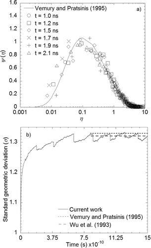
FIG. 2. Variations of (a) average volume-equivalent diameter, and (b) number concentration of particles with time (D_ve), as predicted from the kinetic Monte Carlo simulation and compared with Mukherjee et al. (2003) under the assumption of spherical shape (initial diameter = 1 nm, volume fraction = 10⁻⁶, gas temperature, T_g = 320 K); (c) variation of the average radius of gyration from an experiment (circle) measured by Lattuada et al. (2003) and compared with calculated values (solid line) by current KMC simulation as a function of time, for the polystyrene latex with a primary particle diameter = 72 nm, and a particle volume fraction of 0.0025%.

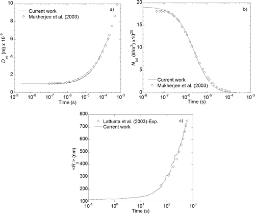
Now we consider kinetic simulation on Brownian aggregation of particles leading to non-spherical aggregates. Starting from polystyrene latex spheres of 250 nm at a volume fraction of 2.5 × 10⁻⁶, average radius of gyration of their fractal-like aggregates is calculated in real time and compared with the results of Lattuada et al.'s experiment in Figure 2c. Even for non-spherical particle growth, it is clearly noted that the present KMC code works well. Henceforth, the growth kinetics and structural characteristics of fractal-like aggregates will be investigated for a wide range of volume fractions.

3.2. Aggregation Kinetics and Transition Behavior of Aggregate Morphology

Figure 3 shows the time variations of total number concentration (N_tot) and average volume-equivalent diameter (D_ve) of particles growing at three different volume fractions (φ) of 0.0005, 0.005, and 0.05 in the free molecular regime at temperature 320 K. It should be noted that the profiles of D_ve and N_tot against time are similar to those in Figures 2a and b, even when the volume fraction φ is increased by several orders of magnitude. It is also observed in Figure 3 that the profiles are both left-shifted in time by almost the same order of magnitude as φ increases, maintaining the shape of the D_ve profile with a slow increase followed by a steep rising. In this figure, we arbitrarily define a characteristics time, t_c,1, for each volume fraction, which is related to the average size and morphology of aggregates. Herein, t_c,1 is defined as the time required for D_ve to reach 2.7 nm corresponding to ⟨N_p⟩ ≈ 20. Though the choice of 2.7 nm has little basis, the time of t_c,1 can characterize the transient coagulation process well with a phenomenological discrimination of critical coagulation stages: particles exhibit the fastest variations in their structures at t ≤ t_c,1 (will be seen). Note that the t_c,1 values are 2 × 10⁻⁸ s, 2 × 10⁻⁹ s, and 1 × 10⁻¹⁰ s for volume fractions of 0.0005, 0.005, and 0.05, respectively. The value of t_c,1 for volume fraction of 0.005 is one tenth of that for volume fraction of 0.0005 as is expected. However, the value of t_c,1 for volume fraction of 0.05 is twice smaller than expected from the case of lower volume fractions. This result suggests that though aggregation is initially presumed in the dilute regime (D_f of 1.8 as will be seen in Figures 4c and 5c), the aggregation at the highest volume fraction seems to be accelerated more than the expectation. This effect is consistent with other previous reports (Fry et al. 2002; Molnar et al. 2012).

FIG. 3. Time variation of number concentration (dashed line with filled symbols) and average volume equivalent diameter of aggregates (solid line with open symbols) as predicted by the KMC simulation for volume fraction of 0.0005 (circle), 0.005 (rectangular), and 0.05 (diamond).

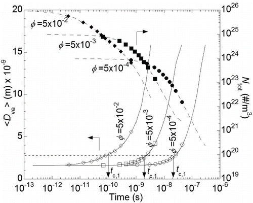
FIG. 4. Variation of D_f (solid line), ⟨C_n⟩ (dashed line), and ⟨A_n⟩ (dotted line) as a function of time for initial volume fraction (φ) of: (a) 0.0005, (b) 0.005, and (c) 0.05.

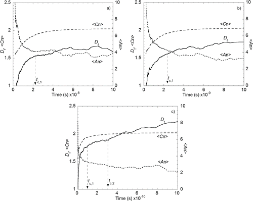
FIG. 5. Time variation of D_f (solid line), average size ⟨R_g⟩ (dashed line), average separation distance between aggregates (⟨R_nn⟩) (dotted line), and the ratio ⟨R_nn⟩ / ⟨R_g⟩ (long and short dashed line) for initial volume fractions (φ) of: (a) 0.0005, (b) 0.005, and (c) 0.05. The D_f represents an average fractal dimension for an ensemble of all aggregates existing at a time, while D_f,large and D_f,small in inset are fractal dimensions obtained for each ensemble of large-scale and small-scale aggregates (refer to Figure 6c).

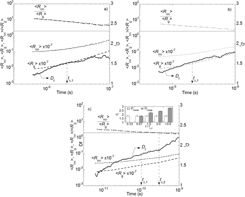
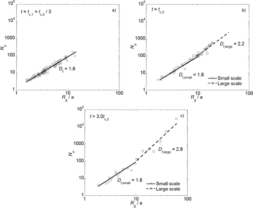
FIG. 6. Log–log plots of number of monomers (N_p) versus radius of gyration normalized by radius of primary particle (R_g/a) of aggregates produced at the volume fraction of 0.05; (a) at early time of t_c,1, (b) at the second characteristic time of t_c,2, and (c) at the final stage (>3t_c,2).

Figures 4a–c shows the time variation of the average fractal dimension (D_f), the average shape anisotropy (⟨A_n⟩), and the average coordination number (⟨C_n⟩) of aggregates for volume fractions of 0.0005, 0.005, and 0.05 at 320 K. At the early stage of aggregation (when t ≤ t_c,1) as shown in Figure 4a, D_f and ⟨C_n⟩ increase most rapidly together with the rapid decrease of ⟨A_n⟩. Then, the three parameters all have minimal change with time, which is indicative of entering a self-similar state: the final stage of the aggregation (Bushell et al. 2002; Fry et al. 2004a,b; Alimova et al. 2009; Heinson et al. 2012). Note that we define another characteristic time, t_c,2, to highlight a sudden increase of the average D_f, particularly at the volume fraction of 0.05 (will be explained more in the next section).

The final value of ⟨C_n⟩ for all volume fractions is 2.0. This value comes from the fact that if a branch is formed (C_n > 2.0), then the coordination number of primary particles at the end of the branch (C_n = 1) will compensate for the increase of average value. In addition, the number of branches with C_n > 2.0 is much smaller than the number of simple bonds with C_n of 2.0. Therefore, the dominant value of coordination number in the aggregate in the absence of restructuring processes is always close to 2.0 (Bushell et al. 2002).

The shape anisotropy tends to decrease down to a final value depending on the volume fraction used. The shape anisotropy values for volume fractions of 0.0005, 0.005, and 0.05 are 4.2, 4.25, and 3.2 at t ≈ t_c,1, and 3.6, 3.2, and 2.2 at the final stage, respectively. These values indicate that the coagulation process for volume fractions of 0.0005 and 0.005 are predominated by more stringy and open aggregates as compared to the case of volume fractions of 0.05. In particular, the final value of shape anisotropy for the volume fraction of 0.0005 agrees well with the value for diffusion-limited coagulation (Fry et al. 2004a,b).

Figures 4a–c also shows the morphology evolution from early time (t < t_c,1) to the end of aggregation: aggregates at early time are widely open and stringy, while aggregates at later time are more compact and less stringy. This fact suggests that aggregation process may increase the average D_f to some values (depending on their volume fraction), rather than decrease the D_f as reported by some previous researchers (Kostoglou and Konstandopoulos 2001; Gruy 2011). Therefore, the purpose of our next study is to investigate how D_f could increase in various volume fractions in the absence of inter-particle potential and to explain the peculiar increase of the average D_f observed at the highest volume fraction as well.

3.3. Effect of Volume Fraction on Transition of Aggregation Regime

Figures 5a–c shows the time variation of D_f and the inter-particle distance between aggregates for volume fractions of 0.0005, 0.005, and 0.05, respectively. In Figure 5a, the average radius of gyration of aggregates, ⟨R_g⟩, for volume fraction of 0.0005 increases from 1 nm up to 10 nm as time elapses, while the inter-particle distance between aggregates, ⟨R_nn⟩, increases relatively slow. Thus, this explains why the ratio ⟨R_nn⟩/⟨R_g⟩ gradually decreases with time. For volume fraction of 0.005, Figure 5b shows quite similar behaviors of ⟨R_g⟩ and ⟨R_nn⟩ to the case of φ = 0.0005, leading to ⟨R_nn⟩/⟨R_g⟩ > 2.0 over the time of interest. These results suggest that coagulation process in this system might occur in the dilute regime (Fry et al. 2004b; Kim and Sorensen 2006).

At the highest volume fraction (φ = 0.05) as shown in Figure 5c, however, ⟨R_nn⟩ no longer remains large in comparison to average size, ⟨R_g⟩. As a result, the ratio ⟨R_nn⟩/⟨R_g⟩ decreases below 2.0 particularly at t > t_c,2, which represents the system moves into the dense regime (Fry et al. 2002; Dhaubhadel et al. 2006, 2009). Recalling that the sudden increase of D_f occurred at t ≈ t_c,2 in Figure 4c, we postulate that a different coagulation mechanism, which could increase the average D_f over 1.8, takes effect at t ≈ t_c,2 and will predominate over the next coagulation.

Note that based on Equation (3)[3] , a single linear fitting was performed for the log–log plot (N_p vs. R_g/a) for an ensemble of aggregates at a time, which could allow an automatic calculation of the average D_f at every time step as shown in Figures 4 and 5. This would make sense only when the aggregates are all characterized with a single value of D_f. As a significant structural change is expected before and after the time of t_c,2 at the highest volume fraction, the size information of the aggregates (N_p vs. R_g) was extracted to test whether the aggregates have a single morphology or not, at five different times of t_c,1, 2t_c,1, 3t_c,1 (= t_c,2), 9t_c,2, and 10t_c,1. For example, Figure 6a shows the log–log plot of aggregates at early time (t = t_c,1); all aggregates are characterized well with a single (average) value of D_f, suggesting that they are still in a dilute regime.

At t = t_c,2, however, the aggregates begin to have two different morphologies with different fractal dimensions of D_f = 1.8 and 2.2, at small size scales and large scales, respectively (Figure 6b). As shown in the figure, the small-scale and large-scale aggregates are discriminated with different symbols of circles and squares, respectively, and their slopes are obtained by a linear least-square fitting for each of groups; D_f,large in the figure represents the fractal dimension for the ensemble of the large-scale aggregates, while D_f,small characterizes the small-scale aggregates. With subsequent increase of time, the D_f,large shows a gradual, but discernible increase, in contrast to the D_f,small which is almost invariant. These behaviors of the fractal dimensions are depicted accordingly in Figure 5c, in addition to the profile of the average D_f. Another thing to note is that the number fraction of large-scale aggregates with D_f,large among the total aggregates increases with time, while that of the small-scale aggregates with D_f,small = 1.8 decreases. This population movement of aggregates, as well as the D_f,large increase and growth of large-scale aggregates, is believed to make the D_f,large dominate the average D_f at later time.

Figure 6c highlights their hybrid structure with D_f,large and D_f,small. The aforementioned population decrease of small-scale aggregates with time indicates that the large-scale aggregates are created as being composed of the small aggregates with lower D_f, This is how the aggregates could preserve the structural nature of their constituent (small-scale). In Figure 6c, the D_f,large of the aggregates increases up to 2.8 at later time (t > 3t_c,2), raising the average D_f to 2.3 at the same time. These findings are summarized in inset of Figure 5c. It should be here noted that previous works on cluster dense systems demonstrated the existence of large superaggregates consisting of open-structured small aggregates (Fry et al. 2004a,b; Kim and Sorensen 2006; Sorensen and Chakrabarti 2011; Kearney and Pierce 2012). Regarding the unique structural property of superaggregates, we believe that our aggregates observed at later time (t > 3t_c,2) in Figures 5c and 6c are the superaggregates. However, there is still another question: how the small-scale aggregates create such compact structures of superaggregates. This issue will be addressed in detail in the next section.

3.4. Effects of Volume Fraction on Coagulation Mechanism

As the structural compactness of aggregates is affected by the position where coagulation occurs (on the edge or in the backbone of targeted aggregate-j), the coagulation position is monitored in terms of its occurrence frequency or probability in a range of time (recall Section 2.6). Figure 7a shows that the probability of coagulation inside targeted aggregate-j (Rs_ic_j/R_g,j < 1.0) tends to increase with volume fraction; this probability also increases with time at a higher volume fraction. At a volume fraction of 0.0005, the inside coagulation probability increases from 7% up to only 17% at t ≤ 2t_c,1 and then becomes almost invariant, suggesting that coagulation mainly occurs outside (rather than inside) aggregate-j without interpenetration. Provided that any self-similar aggregates are attached to the edge of a targeted aggregate, this outside coagulation will not alter the compactness of aggregate in terms of D_f. This inference very likely explains why the inside coagulation probability that was limited to increase at the lowest volume fraction shows a similar behavior to the average D_f in Figure 5a.

FIG. 7. Time variation of two critical probabilities: (a) probability of coagulation inside aggregate-j against time. (b) Probability of P-A coagulation between dissimilar aggregates against time.

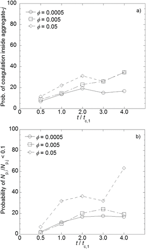
In case of volume fraction of 0.005, the probability increases steadily from 8% up to 34% over the entire time, suggesting that coagulation position gradually shifts from outside to inside aggregate-j. Correspondingly, the average D_f in Figure 5b keeps increasing all the time. Nevertheless, the final value of D_f is not as high as expected from the large increase in the probability. At volume fraction of 0.05, the probability of coagulation inside targeted aggregate-j rapidly increases from 11% to 31% at t ≤ 2t_c,1 and then slightly decreases until t = t_c,2(= 3t_c,1), and then increases again to 35%. The inside coagulation probability at the highest volume fraction is obviously higher than that in either case of lower volume fractions at early time (t ≤ 2t_c,1). However, it is not high enough to explain the sudden increase of the average D_f at t ≈ t_c,2 in Figure 5c. Here, let us recall, from Section 2.6, that the size of colliding aggregate with respect to the targeted aggregate, namely, N_p,i/N_p,j, would be another factor that can affect the aggregates structure.

Figure 7b shows the probability of coagulation between two dissimilar aggregates i and j as a function of time. In case that aggregate-i is much smaller than aggregate-j (N_p,i/N_p,j < 0.1), which is true with a high volume fraction, we could treat the aggregate-i like a primary particle in the view of the aggregate-j, such that the coagulation is categorized to P-A coagulation. The probabilities of P-A coagulation for volume fractions of 0.0005 and 0.005 increase slightly from 2%, and then become steady at 16%–18%, indicating that four out of five coagulations occur between aggregates (A-A) with open structures. Even for the inside coagulation, if a coagulating aggregate-i is similarly large and open structured, this type of coagulation is postulated to play a limited influence on filling the inside of aggregate-j. This might be a reason for the limited increase of the average D_f in Figures 5a and b.

The probability of P-A coagulation for volume fraction of 0.05 increases from 6% to 36% with time at t ≤ 2t_c,1, and then becomes steady until t = t_c,2, and then jumps up to 63% at the later stage (t > 3t_c,2). Note that the inside coagulation probability was also the maximum at that time. From this we conjecture that the coagulation mechanism change from the A-A coagulation to the P-A coagulation allows the primary (relatively small) particles to have no limitation to reach inside large aggregate-j. Therefore, we believe that this coagulation mechanism change, accompanied by the coagulation position shift, relates to the sudden increase of the average D_f from 1.85 to 2.2 at t > t_c,2 as shown in Figure 5c.

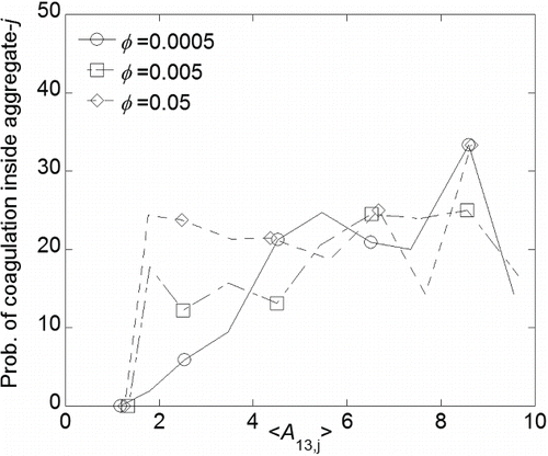
Figure 8 shows the probability of coagulation inside targeted aggregate-j against shape anisotropy value. The probability of interpenetration (Rs_ic_j/R_g,j < 1.0) for volume fraction of 0.0005 smoothly decreases from 25% to zero when the aggregates structure becomes more compact (less anisotropic) with time. Again, we confirm that the elimination of interpenetration supports the limited increase of D_f in the dilute regime. The probability appears to be well correlated with shape anisotropy in the dilute regime (solid line in Figure 8). On the contrary, the probability of Rs_ic_j/R_g,j < 1.0 for volume fractions of 0.05 is almost independent of shape anisotropy. This implies that even while targeted aggregates-j become denser and more isotropic until ⟨A_13,j⟩ ≈ 2.0 with time, a number of small aggregates with D_f,small = 1.8 (seen in Figure 6c) are allowed to penetrate inside the target and complete the P-A coagulation. This might be a sort of driving force for increasing the average D_f over 2.0. When the aggregate becomes too compact (⟨A_13,j⟩ < 2.0), the probability eventually reduces to zero. This denotes that too dense aggregates do not allow any small aggregates to coagulate inside, because only a few of pores are available for interpenetration.

FIG. 8. Relation between the probability of coagulation inside aggregate-j and the shape anisotropy of aggregate-j.

Figures 9a and b show the schematics visually demonstrating coagulation mechanisms for two limiting cases of volume fractions of 0.0005 and 0.05, respectively. Note that all of the aggregates shown in the figures are real snapshots taken during the MC simulations for visualizing morphology of aggregates at significant stages of coagulation. Initially, coagulation at both volume fractions starts from mono-dispersed particles with different separation distances between them. At t < t_c,1 representing the early stage, coagulation occurs in a consecutive way of particle–particle (P-P), particle–aggregate (P-A), and aggregate–aggregate (A-A) coagulations at both volume fractions: P-A coagulation when N_p,i/N_p,j < 0.1 and A-A coagulation if otherwise (see Section 2.6).

FIG. 9. Schematics of time-varying coagulation mechanisms (a) at a volume fraction (φ) of 0.0005, (b) at a volume fraction (φ) of 0.05; the shaded box represents the A-A coagulation, while the white box does the P-A coagulation, and the box size stands for the relative dominance of the P-A or the A-A coagulation; the aggregates are composed of two parts: a large light-gray (green) aggregate-j and the other small dark-gray (blue) aggregate-i, denoting how two particles coagulated; the circle (or a red sphere) represents the position where the coagulation occurs; A_13,j is the anisotropy of aggregate-j before coagulation between i and j.

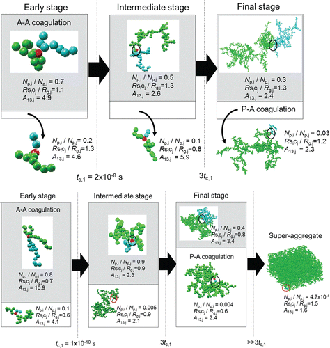
For the volume fraction of 0.0005 in Figure 9a, the ratios of N_p,i/N_p,j and Rs_ic_j/R_g,j are mostly larger than 0.1 and 1.0, respectively, over the entire time considered. Thus, the probability of interpenetration between aggregates becomes insignificant and A-A coagulation mainly occurs as depicted by the box sizes. Even though 16%–18% of coagulations occur inside aggregate-j, the coagulation occurs mainly between open-structured aggregates (D_f ˜ 1.6; ⟨A_n⟩ ˜ 4 from Figure 4a). Such an A-A coagulation limits an increase of the average D_f. Thus, the low volume fraction of 0.0005 leads to A-A coagulation with low probability of interpenetration between aggregates, limiting the transition to the dense regime and resulting in almost constant D_f of 1.7–1.8.

For the volume fraction of 0.05 in Figure 9b, on the other hand, P-A coagulation is not negligible during the entire process of coagulation (Figure 7b). Particularly at t > 3t_c,1 (˜t_c,2), as the P-A coagulation predominates, the P-A coagulation with the highest probability of inter-penetration becomes a major route for the formation of superaggregates. At the same time, even A-A coagulation could occur with the highest interpenetration probability, which makes the overall aggregate structures compact and isotropic at the final stage in Figure 9b. After the aggregates become too large and too compact at the last stage; the ratio of Rs_ic_j/R_g,j and shape anisotropy (A_13,j) of aggregate-j are 1.5 and 1.6, interpenetration process of particles into the compact aggregate is not allowed any more. As such, increasing volume fraction will increase the average D_f to some extent, not continually.

4. CONCLUSION

Artificial aggregates at different volume fractions were generated during aggregation process by using the Kinetic Monte Carlo method. Applying the structure analyses for fractal dimension, coordination number, and shape anisotropy, we found that the aggregates structure in the early stage exhibits a low degree of compactness, and then, the aggregates eventually become more compact in structure along with their growth. At the low volume fraction of 0.0005, the coagulation process followed the DLCA process under the dilute regime, resulting in a typical DLCA structure of D_f = 1.7–1.8. Coagulation at the high volume fraction of 0.05 underwent the regime change from the dilute to dense condition at a certain characteristic time of t_c,2. As a result, the aggregates at early time of t < t_c,2 preserved their dilute-limit fractal dimension of 1.8. At t > t_c,2, on the other hand, the aggregates underwent a gradual structural transformation from the dilute-limit open structure to the hybrid structure of superaggregates. This distinct regime change of coagulations was investigated in detail in terms of probabilities of interpenetration, and P-A or A-A coagulation. At the low volume fraction, the coagulation was predominated by the A-A coagulation with rare interpenetration, resulting in D_f < 1.85 as in the dilute limit. At the highest volume fraction, coagulation occurred in two subsequent steps: typical A-A coagulation in dilute regime at the early stage followed by the P-A coagulation with the highest probability of interpenetration at the later stage (at t > t_c,2). This was proposed as a main route for creation of the superaggregates at the dense condition.

Funding

This work was supported by the National Research Foundation of Korea (NRF) grant funded by Ministry of Science, ICT and Future Planning (MSIP) (No. 2010-0019543); also by the Global Frontier R&D Program on Center for Multiscale Energy System funded by the National Research Foundation under the MSIP (No. 2012M3A6A7054863), and by the MSIP and National Research Foundation (NRF) of Korea (2014M3C8A5030614).

REFERENCES

- Alimova, A., Katz, A., Orozco, J., Wei, H., Gottlieb, P., Rudolph, E., Steiner, J.C., and Xu, M. (2009). Broadband Light Scattering Measurements of the Time Evolution of the Fractal Dimension of Smectite Clay Aggregates. J. Opt. A- Pure Appl. Opt., 11:105706–105712.
- Brasil, A. M., Farias, T. L., Carvalho, M. G., and Koylu, U. O. (2001). Numerical Characterization of the Morphology of Aggregated Particles. Aerosol Sci. Technol., 32:489–508.
- Buesser, B., Heine, M. C., and Pratsinis, S. E. (2009). Coagulation of Highly Concentrated Aerosols. Aerosol Sci. Technol., 40:89–100.
- Bushell, G. C., Yan, Y. D., Woodfield, D., Raper, J., and Amal R. (2002). On Techniques for the Measurement of the Mass Fractal Dimension of Aggregates. Adv. Colloid Interface Sci., 95:1–50.
- Chakrabarty, R. K., Moosmuller, H., Arnott, W. P., Garra, M. A., Tian, G. X., Slowik, J. G., Cross, E. S., Han, J. H., Davidovits, P., Onasch, T. B., and Warsnop, D. R. (2009). Low Fractal Dimension Cluster-Dilute Soot Aggregates From a Premixed Flame. Phys. Rev. Lett., 102:235504.
- Dhaubhadel, R., Chakrabarti, A., and Sorensen, C. M., (2009). Light Scattering Study of Aggregation Kinetics in Dense, Gelling Aerosols. Aerosol Sci. Technol., 43:1053–1063.
- Dhaubhadel, R., Pierce, F., Chakrabarti, A., and Sorensen, C. M. (2006). Hybrid Superaggregate Morphology as a Result of Aggregation in a Cluster-Dense Aerosol. Phys. Rev. E, 73:011404.
- Evans, W., Prasher, R., Fish, J., Meakin, P., Phelan, P., and Keblinski, P. (2008). Effect of Aggregation and Interfacial Thermal Resistance on Thermal Conductivity of Nanocomposites and Colloidal Nanofluids. Int. J. Heat Mass Transfer, 51:1431–1438.
- Fry, D., Chakrabarti, A., Kim, W., and Sorensen, C. M. (2004a). Structural Crossover in Dense Irreversibly Aggregating Particulate Systems. Phys. Rev. E, 69:061401.
- Fry, D., Mohammad, A., Chakrabarti, A., and Sorensen, C. M. (2004b). Cluster Shape Anisotropy in Irreversibly Aggregating Particulate Systems. Langmuir, 20:7871–7879.
- Fry, D., Sintes, T., Chakrabarti, A., and Sorensen, C. M. (2002). Enhanced Kinetics and Free-Volume Universality in Dense Aggregating Systems. Phys. Rev. Lett., 89:148301.
- Gimel, J. C., Nicolai, T., and Durand, D. (1999). 3D Monte Carlo Simulations of Diffusion Limited Cluster Aggregation up to the Sol-Gel Transition: Structure and Kinetics. Sol-Gel Sci. Technol., 15:129–136.
- Gruy, F. (2011). Population Balance for Aggregation Coupled with Morphology Changes. Colloids Surf. A-Physicochem. Eng. Aspects, 374:69–76.
- Hasmy, A., Anglaret, E., Thouy, R., and Jullien, R. (1997). Fluctuating Bond Aggregation: A Numerical Simulation of Neutrally-Reacted Silica Gels. J. Phys. I, 7:521–542.
- Heine, M. C.. and Pratsinis, S. E. (2006). Brownian Coagulation in Dense Systems: Thermal Non-equilibrium Effects. Langmuir, 22:10238–10245.
- Heinson, W. R., Sorensen, C. M., and Chakrabarti, A. (2010). Does Shape Anisotropy Control the Fractal Dimension in Diffusion-Limited Cluster-Cluster Aggregation? Aerosol Sci. Technol., 44:12i–12iv.
- Heinson, W. R., Sorensen, C. M., and Chakrabarti, A. (2012). A Three Parameter Description of the Structure of Diffusion Limited Cluster Fractal Aggregates. J. Colloid Interface Sci., 375:65–69.
- Jullien, R., and Meakin, P. J. (1989). Simple Models for the Restructuring of Three-Dimensional Ballistic Aggregates. J. Colloid Interface Sci., 127:265–272.
- Kearney, S. P., and Pierce, F. (2012). Evidence of Soot Superaggregates in a Turbulent Pool Fire. Combust. Flame, 159:3191–3198.
- Kim, S., Lee, K.-S., Zachariah, M. R., and Lee, D. (2010). Three Dimensional Off-Lattice Monte Carlo Simulations on a Direct Relation Between Experimental Parameters and Fractal Dimension of Colloidal Aggregates. J. Colloid Interface Sci., 344:353–361.
- Kim, W. G., and Sorensen, C. M. (2006). Soot Aggregates, Superaggregates and Gel-Like Networks in Laminar Diffusion Flames. J. Aerosol Sci., 37:386–401.
- Kostoglou, M., and Konstandopoulos, A. G. (2001). Evolution of Aggregate Size and Fractal Dimension During Brownian Coagulation. J. Aerosol Sci., 32:1399–1420.
- Lattuada, M. (2012). Predictive Model for Diffusion-Limited Aggregation Kinetics of Nanocolloids Under High Concentration. J. Phys. Chem. B, 116:120–129.
- Lattuada, M., Wu, H., and Morbidelli, M. (2003). A Simple Model for the Structure of Fractal Aggregates. J. Colloid Interface Sci., 268:106–120.
- Liffman, K. (1992). A Direct Simulation Monte-Carlo for Cluster Coagulation. J. Comput. Phys., 100:116–127.
- Lindsay, H. M., Klein, R., Weitz, D. A., Lin, M. Y., and Meakin, P. (1989). Structure and Anisotropy of Colloid Aggregates. Phys. Rev. A, 39:3112–3119.
- Madler, L., Lall, A. A., and Friedlander, S. K. (2006). One-step Aerosol Synthesis of Nanoparticle Agglomerate Films: Simulation of Film Porosity and Thickness. Nanotechnology, 17:4783–4795.
- Mansfield, M. L.. and Douglas, J. F. (2013). Shape Characteristics of Equilibrium and Non-Equilibrium Fractal Clusters. J. Chem. Phys., 139:044901.
- Mazumdar, T., Mazumder, S., and Sen, D. (2011). Temporal Evolution of Mesoscopic Structure of Some Non-Euclidean Systems Using a Monte Carlo model. Phys. Rev. B, 83:104302.
- Molnar, D., Mukherjee, R., Choudhury, A., Mora, A., Binkele, P., Selzer, M., Nestler, B., and Schmauder, S. (2012). Multiscale Simulations on the Coarsening of Cu-rich Precipitates in a-Fe Using Kinetic Monte Carlo, Molecular Dynamics and Phase-field Simulations. Acta Mater., 60:6961–6971.
- Mukherjee, D., Sonwane, C. G., and Zachariah, M. R. (2003). Kinetic Monte Carlo Simulation of the Effect of Coalescence Energy Release on the Size and Shape Evolution of Nanoparticles Grown as an Aerosol. J. Chem. Phys., 119:3391–3404.
- Orrite, S. D., Stoll, S., and Schurtenbergerb, P. (2005). Off-lattice Monte Carlo Simulations of Irreversible and Reversible Aggregation Processes. Soft Matter., 1:364–371.
- Reim, M., Korner, W., Manara, J., Korder, S., Arduini-Schuster, M., Ebert, H.-P., and Fricke, J. (2005). Silica Aerogel Granulate Material for Thermal Insulation and Daylighting. Solar Energy, 79:131–139.
- Rottereau, M., Gimel, J. C., Nicolai, T., and Durand, D. (2004). Monte Carlo Simulation of Particle Aggregation and Gelation: I. Growth, Structure and Size Distribution of the Clusters. Eur. Phys. J. E, 15:133–140.
- Sanz, E.. and Marenduzzo, D. (2010). Dynamic Monte Carlo Versus Brownian Dynamics: A Comparison for Self-diffusion and Crystallization in Colloidal Fluids. J. Chem. Phys., 132:194102.
- Smith, M.. and Matsoukas, T. (1998). Constant-Number Monte Carlo Simulation of Population Balances. Chem. Eng. Sci., 53:1777–1786.
- Soos, M., Lattuada, M., and Sefcik, J. (2009). Interpretation of Light Scattering and Turbidity Measurements in Aggregated Systems: Effect of Intra-Cluster Multiple-Light Scattering. Phys. Chem. B, 113:14962–14970.
- Sorensen, C. M., and Chakrabarti, A. (2011). The Sol to Gel Transition in Irreversible Particulate Systems. Soft Matter., 7:2284–2296.
- Sorensen, C. M., and Roberts, G. C. (1997). The Prefactor of Fractal Aggregates. J. Colloid Interface Sci., 186:447–452.
- Tassopoulos, M., and Rosner, D. E. (1992). Microstructural Descriptors Characterizing Granular Deposits. AIChE J., 38:15–25.
- Trzeciak, T. M. (2012). Brownian Coagulation at High Particle Concentrations, Ph. D. thesis. Delft University of Technology, Delft, p. 28, http://repository.tudelft.nl/view/ir/uuid:92c8f6b3-feab-4dac-bc0a-db0c4460870f.
- Trzeciak, T. M., Podgórski, A., and Marijnissen, J. C. M. (2014). Brownian Coagulation in Dense Systems: Thermal Non-equilibrium Effects. J. Aerosol Sci., 69:1–12
- Vemury, S.. and Pratsinis, S. E. (1995). Self-Preserving Size Distributions of Agglomerates. J. Aerosol Sci., 26:175–185.
- Wu, M. K., and Friedlander, S. K. (1993). Enhanced Power Law Agglomerate Growth in the Free Molecule Regime. J. Aerosol Sci., 24:273–282.
- Wu, H., Lattuada, M., and Morbidelli, M. (2013). Dependence of Fractal Dimension of DLCA Clusters on Size of Primary Particles. Adv. Colloid Interface Sci., 195–196:41–49.
- Yang, G., and Biswas, P. (1999). Computer Simulation of the Aggregation and Sintering Restructuring of Fractal-Like Clusters Containing Limited Numbers of Primary Particles. J. Colloid Interface Sci., 211:142–150.