Field intercomparison of the gas/particle partitioning of oxygenated organics during the Southern Oxidant and Aerosol Study (SOAS) in 2013

ABSTRACT

We present results of the first intercomparison of real-time instruments for gas/particle partitioning of organic species. Four recently-developed instruments that directly measure gas/particle partitioning in near-real time were deployed in Centreville, Alabama during the Southern Oxidant Aerosol Study (SOAS) in 2013. Two instruments were filter inlet for gases and aerosols high-resolution chemical ionization mass spectrometers (FIGAERO-HRToF-CIMS) with acetate (A-CIMS) and iodide (I-CIMS) ionization sources, respectively; the third was a semi-volatile thermal desorption aerosol GC-MS (SV-TAG); and the fourth was a high-resolution thermal desorption proton-transfer reaction mass spectrometer (HR-TD-PTRMS). Signals from these instruments corresponding to several organic acids were chosen for comparison. The campaign average partitioning fractions show good correlation. A similar level of agreement with partitioning theory is observed. Thus the intercomparison exercise shows promise for these new measurements, as well as some confidence on the measurement of low versus high particle-phase fractions. However, detailed comparison show several systematic differences that lie beyond estimated measurement errors. These differences may be due to at least eight different effects: (1) underestimation of uncertainties under low signal-to-noise; (2) inlet and/or instrument adsorption/desorption of gases; (3) differences in particle size ranges sampled; (4) differences in the methods used to quantify instrument backgrounds; (5) errors in high-resolution fitting of overlapping ion groups; (6) differences in the species included in each measurement due to different instrument sensitivities; and differences in (7) negative or (8) positive thermal decomposition (or ion fragmentation) artifacts. The available data are insufficient to conclusively identify the reasons, but evidence from these instruments and available data from an ion mobility spectrometer shows the particular importance of effects 6–8 in several cases. This comparison highlights the difficulty of this measurement and its interpretation in a complex ambient environment, and the need for further improvements in measurement methodologies, including isomer separation, and detailed study of the possible factors leading to the observed differences. Further intercomparisons under controlled laboratory and field conditions are strongly recommended.

Copyright © 2017 American Association for Aerosol Research

EDITOR:

• Paul Ziemann

1. Introduction

Atmospheric aerosols have important effects on human health (Pope et al. 2009), visibility (Watson 2002), and the Earth's climate (Stocker et al. 2013). Aerosols affect climate directly by scattering or absorbing light and indirectly by altering cloud brightness, lifetime, and precipitation (Stocker et al. 2013). Recently, a long-term impact of aerosols on biogeochemical cycles has also been proposed with a radiative forcing comparable to that of the aerosol direct effect (Mahowald 2011). Submicron particles are the more active climatically and most important for human health impact, and organic aerosols (OA) represent a substantial fraction of their mass (Kanakidou et al. 2005; Zhang et al. 2007; Jimenez et al. 2009).

OA can be classified into primary OA (POA) that is directly emitted by both natural and anthropogenic sources and secondary OA (SOA) that is formed by oxidation of gas-phase compounds followed by the gas-to-particle partitioning of less volatile products (Pankow 1994; Donahue et al. 2006; Jimenez et al. 2009) or by aqueous-phase chemistry (Lim et al. 2010; Ervens 2015). Studies have demonstrated that a major fraction of OA is SOA across urban, rural and remote sites (de Gouw 2005; Hallquist et al. 2009; Jimenez et al. 2009). The formation, aging, chemical properties, and lifetime of OA are not well understood (Goldstein and Galbally 2007; de Gouw and Jimenez 2009; Hallquist et al. 2009), and these large uncertainties often lead to discrepancies between models and measurements of aerosol loading (de Gouw 2005; Volkamer et al. 2006; Dzepina et al. 2009; Tsigaridis et al. 2014).

SOA has been long assumed to be semivolatile (Odum et al. 1996). In the last few years, however, several studies have suggested that some of the model-measurement discrepancies might be due to nonequilibrium gas/particle partitioning caused by kinetic limitations due to the presence of glassy or semi-solid phases (Vaden et al. 2010, 2011; Virtanen et al. 2010). Whether and when such limitations apply is a focus of present research (Virtanen et al. 2010; Vaden et al. 2010, 2011; Shiraiwa et al. 2011; Perraud et al. 2012; Price et al. 2013; Renbaum-Wolff et al. 2013; Saleh et al. 2013; O'Brien et al. 2014; Yatavelli et al. 2014a,b; Upshur et al. 2014; Lopez-Hilfiker et al. 2016). To better understand and predict formation, growth, evolution, and losses of SOA, it is critical to understand gas/particle partitioning of organic species in the real atmosphere. Most studies to date addressing the kinetic limitations to partitioning have been indirect methods and without chemical specificity. Accurate, direct, and fast time-resolution measurements of the gas/particle partitioning of key OA species are needed to resolve these discrepancies and improve the representation of OA in atmospheric models.

Recently the direct in situ measurement of the gas/particle partitioning of organic species and/or groups of species has become possible due to new instrumental developments (Holzinger et al. 2010; Yatavelli and Thornton 2010; Yatavelli et al. 2012; Lopez-Hilfiker et al. 2013; Rollins et al. 2013; Isaacman et al. 2014). However, different measurements of gas and particle-phase at the same time by the same instrument (and therefore F_p) have not been previously compared.

Semivolatile organic acids are abundant in the atmosphere (Chebbi and Carlier 1996; Yatavelli et al. 2015) and are important oxidation products of anthropogenic and biogenic volatile organic compounds (VOC) and contribute to SOA (Veres et al. 2011; Andrews et al. 2012; Vogel et al. 2013). Because of their vapor pressure range, many larger or more oxidized organic acids are expected to partition between the gas and particle phases at typical atmospheric OA concentrations (∼0.1–100 µg m⁻³). However, despite their ubiquity and importance, the gas/particle partitioning dynamics and equilibria of organic acids are still poorly characterized.

Here, we compare results from four instruments that directly measured gas/particle partitioning of organic acids with high time resolution. Measurements were conducted at the ground supersite during the 2013 SOAS field study in the southeastern United States (Hu et al. 2015; Carlton et al. 2016). To our knowledge, this is the first intercomparison of real-time gas/particle partitioning to date, whether in a field or laboratory setting.

2. Instrumentation and methods

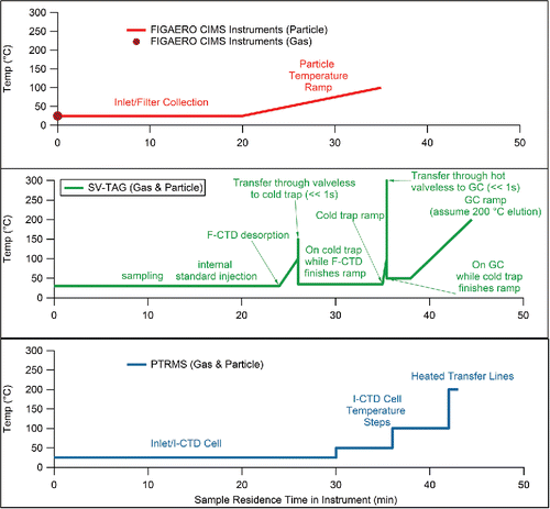
Four instruments are compared in this study: two filter inlet for gases and aerosols (FIGAERO) high-resolution–time-of-flight–chemical-ionization mass spectrometers (HRToF-CIMS) operated by different research groups and with different ionization methods, a semi-volatile thermal-desorption aerosol gas chromatograph (SV-TAG), and a high-resolution–thermal-desorption–proton-transfer-reaction mass spectrometer (HR-TD-PTRMS). All four instruments measure partitioning by separating particle-phase compounds from gas- or gas-plus-particle-phase compounds during sampling and using thermal desorption to evaporate particle-phase compounds. Either online analysis (without heating) or thermal desorption are used to analyze gas-phase compounds. Details about each instrument can be found below and a diagram of the respective heating profiles experienced by a typical compound (desorbing at 100°C) is shown in Figure 1. For the CIMS instruments, the temperature ramp acts such that the molecules do not encounter a temperature greater than their thermal desorption temperature, decreasing the likelihood of thermal decomposition. In the PTRMS (which uses heated transfer lines) and the SV-TAG (which uses a temperature ramp to facilitate flow through the GC column and temperatures up to 250°C for rapid flow through valves) higher temperatures are experienced before detection. That might increase the chances of thermal decomposition, although the residence times and materials that the species come into contact in the different instruments likely also play a role. As exposure to higher temperatures in SV-TAG is dominated by the temperature ramp of the GC, decomposition in this instrument is expected to be similar to most other, more common chromatographic analyses of the studied compounds, such as filter collection and extraction. It has been shown that some isoprene SOA oligomers do decompose in the FIGAERO-CIMS at temperatures below 100°C, therefore decomposition is not only a high temperature process (Lopez-Hilfiker et al. 2016). No drying of gas-phase water was carried out for any instrument. A summary of each instrument's separation and detection method can be found in Table S1.

Figure 1. Schematic diagram of the temperature profiles that a typical compound would experience in the gas and particle phase in each instrument. The example compound is assumed to have a volatility such that it would thermally desorb at 100°C. The width of the thermal desorption curve (Faulhaber et al. 2009; Lopez-Hilfiker et al. 2016) is ignored for the purposes of this diagram.

2.1. Figaero-HRToF-CIMS

Two of the instruments compared in this study use two versions of the same gas/particle inlet, followed by detection with acetate (A-CIMS) or iodide (I-CIMS) reagent ions. These instruments were built by Aerodyne, with custom modifications by the research groups. The key components of this instrument are described in detail elsewhere (Yatavelli et al. 2012, 2014a; Lopez-Hilfiker et al. 2013). Briefly, it is composed of three stages. The first stage is the filter inlet for gases and aerosols (FIGAERO), a dual parallel inlet (one for gas and one for aerosol) that was designed to simultaneously sample atmospheric gases and aerosols on a semi-continuous basis (Lopez-Hilfiker et al. 2013). The inlet switches between different modes to measure gas and particle phase compounds. In the “sampling” mode, ambient air is drawn through the gas phase inlet and gases are analyzed, while aerosols are simultaneously collected on a PTFE Teflon-membrane filter. During the “desorption mode,” both atmospheric sampling flows are still drawn through their inlets at the same rates (to avoid transient losses/sources in both inlets due to inlet adsorption/desorption if the flow was interrupted), but are bypassed directly into the pumps at the latest possible point before entering the instrument. Meanwhile the aerosols are thermally desorbed off the filter and sampled into the instrument. Aerosol desorption is accomplished by heating ultra-high purity (UHP) nitrogen (N₂) at a steady ramp rate of 17°C per min up to 200°C while flowing it over the filter for 10 min (times in this section apply to the A-CIMS, small differences for the I-CIMS are summarized below). The N₂ flow is then held at 200°C for 20 additional min to ensure that all organic material is removed from the filter and reduce any carry-over for the next collection/desorption cycle. Finally, room-temperature N₂ is passed over the filter for 5 min to cool the filter and its enclosure before initiating the next aerosol collection cycle. This entire cycle is repeated continuously every 55 min. Every 6th cycle is a “zero cycle,” where UHP nitrogen is sampled through the gas inlet and a filter is placed in front of the particle phase inlet, using the same timing as described above for the ambient measurements, in order to regularly quantify the instrument and inlet backgrounds for both modes of operation. Figure S1 shows an example of the signals observed over a whole cycle for the A-CIMS.

The second stage of the instrument is the chemical ionization region (also known as ion-molecule reaction region, IMR). Chemical ionization (CI) enables sensitive and selective detection of targeted compounds. This region was operated with either acetate reagent ion or iodide reagent ion and is described in the following sections.

The third stage is the high-resolution–time-of-flight mass spectrometer (H-TOF, Tofwerk AG, Thun, Switzerland), which rapidly (33 kHz averaged to 1 s) acquires the entire mass spectrum. The high resolving power (R > 4000 FWHM at m/z 300 in V ion-path mode as used here) of this stage allows for estimation of the elemental composition of many of the measured compounds (DeCarlo et al. 2006; Yatavelli et al. 2012). Only the elemental composition of the analyte can be determined using this method, while structural isomers cannot be distinguished. In addition the instrument resolution is not sufficient to resolve all possible ions that could be present, which introduces some ambiguity in the analysis, especially for small peaks in a isobaric peak ensemble (Stark et al. 2015). The A-CIMS is first described in detail, while the description of the I-CIMS summarizes the key differences with the A-CIMS.

2.1.1. Acetate CIMS

Two inlet configurations were used for this instrument. In the first configuration during “sampling” mode, ambient air was drawn at 10 standard liters per minute (slpm, 273 K and 1 atm) through a 6 m long, 0.95 cm inner diameter PTFE Teflon tube and then subsampled at the instrument entrance at 2 slpm, with a total inlet residence time of 2.5 s. Gas-phase species are analyzed continuously during the sampling phase. There is no filtering of particles in this inlet, but evaporation of particle phase compounds is thought to not contribute substantially to gas phase signal due to low residence time of particles in the IMR (Yatavelli and Thornton 2010; Lopez-Hilfiker et al. 2013). Molecules evaporating from particles deposited to the IMR surfaces should be approximately taken into account by the background subtraction process. Simultaneously, aerosols were sampled through a PM_2.5 cyclone at 10 slpm through a 0.95 cm inner diameter copper tube, also approximately 6 m in length, with an inlet residence time of 2.5 s, and collected for 20 min on a PTFE Teflon-membrane filter. Both inlets sampled from approximately 6 meters off the ground. A picture of the inlet can be found in Figure S2. A second inlet configuration was implemented on 5 July 2013 to allow for much shorter inlet lengths and reduce the potential importance of inlet adsorption and memory effects. Results from both inlets are compared below and show little difference. All data intercompared with other instruments from A-CIMS in this article uses the first configuration, due to the timing of when the different instruments were operating simultaneously.

Acetate ions [CH₃C(O)O⁻] abstract a proton from organic acids, typically without (or with limited) fragmentation, or form ion-molecule adducts. This CI method is discussed in detail elsewhere (Veres et al. 2008; Bertram et al. 2011; Yatavelli et al. 2012). In the chemical ionization region, 2 slpm of sample gas is mixed at a 90 degree angle with a 2 slpm flow containing the reagent ions. Acetate reagent ions are formed by flowing 2 slpm UHP N₂ containing acetic anhydride (from bubbling the N₂ through liquid acetic anhydride) which then pass through a Po-210 ionizer (10 mCi). A residence time of ∼100 ms in the CI region allows for the reagent ion/sample molecule reactions to proceed (∼85 mbar). 0.5 slpm is pulled into the mass spectrometer through a critical orifice, while the rest of the flow is exhausted through a pump. Due to the selective chemical ionization scheme used, most molecules detected are assumed to be acids (Veres et al. 2008).

All data were processed using the custom Tofware software package (version 2.4.3; Tofwerk AG, Thun, Switzerland; Aerodyne Research Inc., Billerica, MA, USA) (Stark et al. 2015) within Igor Pro (version 6.32; Wavemetrics, Inc., Lake Oswego, OR, USA). Example data, including a zero cycle to show the backgrounds of the instrument, can be found in Figure S1. Figure S3 shows how the FIGAERO is calibrated by integrating the total thermal desorption signal which led to repeatable, linear calibrations.

2.1.2. I-CIMS

This instrument is conceptually identical to the one described above except for the reagent ion. This instrument uses the iodide ion, I⁻, as a reagent ion to selectively ionize relatively oxidized molecules starting from CH₃I precursor (Huey et al. 1995; Aljawhary et al. 2013; Lee et al. 2014). The instrument was used with a FIGAERO collector and high-resolution mass spectrometer in the same way as the A-CIMS was described above. The two FIGAERO collectors were built separately following the same design (by UW for the I-CIMS and by Aerodyne/Colorado for the A-CIMS). The stainless steel 25 mm OD particle phase inlet for the I-CIMS was 2.7 m long and used a custom inertial impactor with a 2 μm cutpoint. The PTFE gas phase inlet (19.05 mm OD) was 1.8 m long. Flow rates were 15.5 slpm for the gas phase and 22 slpm for the particle phase inlet. With the I-CIMS, sampling time was kept at 20 min and the desorption phase at 45 min, with 20 min temperature ramp to 200°C, 20 min soaking at 200°C, and 5 min cooling down to ambient temperature. The sensitivity using this ion chemistry is dependent on water concentration in the chemical ionization region. Since the gas phase is sampled at ambient RH and the particle phase is sampled using dry nitrogen, a sensitivity correction was applied to account for the effect of water (Lee et al. 2014).

2.2. SV-TAG

A dual-cell semivolatile thermal desorption aerosol gas chromatograph (SV-TAG) with in situ derivatization provided hourly measurement of functionalized semi- and low-volatility organic compounds in the gas- and particle-phases. A detailed description of this instrument has been provided elsewhere (Isaacman et al. 2014), and is only briefly summarized here. Sample air is drawn through an inlet and into two identical custom made filter cells for collection and thermal desorption (F-CTD cells), which are collected at the same time, and then analyzed in series. The inlet comprises 2 stages: a “chimney” followed by a sub-sample line off the center stream. Air is pulled at ∼200 slpm through a 38.7 cm wide cleaned steel duct (“chimney”) from a height of ∼4 m above ground (residence time ∼10–15 s). The SV-TAG subsamples at 20 slpm (10 for each cell) from the center stream of the chimney through a cyclone with a size cutoff of 1 μm followed by ∼1 m of 0.95 cm (3/8′) ID clean stainless steel (SS) tubing. Each F-CTD cell consists of a high-surface-area passivated SS metal fiber filter (Zhao et al. 2013) in a thermally-controlled housing (30°C), which quantitatively collects gas and particle-phase compounds with a volatility as high as that of tetradecane (saturation concentration at 25°C, C* ∼ 10⁷ µg m⁻³) (Zhao et al. 2013). During sample collection, one cell samples through a 400-channel cylindrical activated-carbon denuder (30 mm OD × 40.6 mm length; MAST Carbon) to remove gas-phase species. Simultaneous collection of total (undenuded) and particle-only (denuded) samples, followed by sequential analysis of the samples and subtraction to calculate gas concentrations, allows a direct calculation of gas/particle partitioning of the measured species. Calibration occurred through several injections per day of varying concentrations of liquid standards, and an internal standard was added to every sample to control for run-to-run variability in instrument response. Background and zero corrections occurred through both regular sampling of N₂ to measure gas-phase artifacts from sample lines, and analysis of F-CTD cells with no sample collection to confirm instrument zeros. Penetration of gas-phase species through the denuder was tested approximately weekly by placing a PTFE Teflon filter in the sampling line upstream of the denuder, and found to be negligible in most cases. In the cases where it was not negligible it was corrected for through the background subtraction.

A typical duty cycle consists of 22 min of sampling on both cells, injection of standards (2 min), two-step purge-and-trap desorption (30 to 310°C, 16 min) and chromatographic analysis (14 min: 50 to 330°C at 23.6°C/min, 2 min hold) of F-CTD1, and then desorption of F-CTD2 (16 min), and chromatographic analysis while collection of the subsequent sample begins after exactly 60 min from the previous collection start. During analysis, samples are thermally desorbed into a helium purge flow saturated with derivatizing agent (MSTFA, N-Methyl-N-(trimethylsilyl)-trifluoroacetamide) in a two-step purge-and-trap method. Conversion of hydroxyl groups into silyl ethers and esters using MSTFA during the first stage of desorption allows quantitative analysis of highly polar compounds by gas chromatography/mass spectrometry (GC/MS). Analysis was performed using a custom-modified 7890A gas chromatograph (Agilent Technologies) equipped with a nonpolar column (20 m × 0.18 mm × 0.18 um, Rxi-5Sil MS; Restek, Bellefonte, PA, USA) coupled to a 5975C unit-resolution quadrupole mass spectrometer (Agilent Technologies). All chromatographic data were reduced and analyzed using custom analysis code written in Igor Pro 6.3 (WaveMetrics), which forms the basis of the publicly available software TAG ExploreR and iNtegration (Isaacman-VanWertz G, Sueper D (2014) TERN: TAG ExploreR and iNtegration. Available at: https://sites.google.com/site/terninigor).

2.3. HR-TD-PTRMS

This instrument (hereinafter “PTR-MS” for short) consists of a modified-commercial PTR-MS instrument (PTR-TOF8000, Ionicon Analytik GmbH, Innsbruck, Austria) with a high mass-resolution time-of-flight mass spectrometer (H-TOF, Tofwerk AG, Thun, Switzerland, same TOF analyzer used by A-CIMS and I-CIMS) with separate gas and aerosol inlets. The aerosol samples were collected through dual aerosol inlet (copper tubing of height ∼ 4m and ID ∼0.65 cm). The details of the aerosol sampling inlet, collection and analytical methods can be found in Holzinger et al. (2010). In the aerosol collection channel, particles in the size range 0.07–2 μm were collected by impaction on a collection-thermal-desorption (I-CTD) cell. Aerosols collected from a total volume of 150–220 liters of air were desorbed from the I-CTD cell into a UHP N₂ flow of 7 mL min⁻¹. Thermal desorption increased the temperature in 7 steps of 50°C increments to a maximum of 350°C with a ramp and dwell time of 3 min per step followed by an oxidizing step for 3 min during which UHP N₂ was replaced by synthetic air. The N₂ with the desorbed aerosol species was analyzed with the PTR-MS. All transfer lines to the PTR-MS were made of Sulfinert-coated (Restek) stainless steel and were heated continuously (200°C) to avoid re-condensation of evaporated organic material. Gas sample was drawn at 1 slpm through ∼20 cm of ∼0.65 cm ID Silcosteel tube (Restek) from the center airstream of the chimney (steel duct of length ∼4 m and ID ∼ 38 cm, airflow ∼200 slpm) which was then passed through a custom-made sampler box containing 3 denuders in series to sample gas-phase species: 1^st denuder DB-1 column, 0.53 mm × 5.0 μm for capturing semivolatile organic compounds (SVOCs), 2nd denuder DB-1 column, 0.53 mm × 5.0 μm for capturing any leftover SVOCs, and 3^rd denuder- activated carbon for capturing VOCs. SVOCs and VOCs are sampled through the denuder box for 30 min. After sampling, a reverse flow of UHP N₂ (70 sccm) was applied, and the PTRMS sampled the effluent N₂ from the denuder system containing the sampled molecules. Each denuder was heated by ramping the temperature up to 200°C in four steps of 50°C with a ramp and hold time of 4 min per step followed by an oxidizing step for 3 min. The sampler box was then cooled to room temperature, to minimize volatilization of the SVOCs during sampling and protect the collection system from environmental changes. Gas-phase backgrounds were measured every 9 h by sampling ambient air through a platinum catalyst at 500°C, while aerosol backgrounds (sampling through a PTFE Teflon membrane filter, Zefluor 2.0 μm, Pall Corp., New York, NY, USA) were measured every other measurement cycle. A total of 12–13 measurement cycles were performed per day. Each cycle was completed in 107 min and included the analysis of the first I-CTD cell aerosol samples (25 min), second I-CTD cell aerosol samples (background) (25 min), and the denuder gas samples (57 min). All data were processed using the PTRwid software following Holzinger (2015).

2.4. Nitrate-ion ion mobility time-of-flight mass spectrometer (NO₃⁻-IMS-TOF)

In order to gain more information about the presence of isomers, ion mobility-mass spectrometry (Eiceman and Karpas 2010) measurements were obtained from a drift-tube ion mobility spectrometer coupled to an H-TOF high-resolution time-of-flight mass spectrometer (IMS-TOF; Tofwerk AG, Thun, Switzerland). The instrument has been described in detail in previous publications (Kaplan et al. 2010; Zhang et al. 2014b; Krechmer et al. 2016). The IMS-TOF was deployed during SOAS with a custom-built nitrate-ion (NO₃⁻) chemical ionization source initiated with an X-ray ionizer (Hamamatsu Photonics, Hamamatsu, Japan). Data were post-processed and analyzed using the Tofware IMS data analysis package for Igor Pro. Additional results from the IMS-TOF at the SOAS site are described in (Krechmer et al. 2016). We note that due to the different ion chemistries and inlet configurations, the species detected with the IMS-TOF may not completely overlap with those detected by the other instruments.

2.5. Gas/particle partitioning calculations

All gas/particle partitioning measurements are expressed as fractions of a given species (i) in the particle phase (F_p,i), calculated as the ratio of the measured particle-phase concentration to the measured total concentration (gas plus particle) after subtraction of any instrument backgrounds, i.e.:[1]

2.6. Uncertainty estimation

Measurement uncertainties were estimated for each instrument based on its particular measurement method. Note that the estimated errors do not include uncharacterized errors that may be factors such as interfering isomers, thermal decomposition, oligomer interference, or any uncharacterized sampling artifacts. For A-CIMS and I-CIMS, the total uncertainty is calculated as the combination of the estimated accuracy and precision:[2]

Particle and gas-phase signals are calculated for the CIMS instruments as[3]

Each of the three components (signal, background, and sensitivity, for the gas and particle phase measurements) has an accuracy and a precision, resulting in up to 12 components contributing to the overall F_p uncertainty. The estimation methods for each of these 12 components can be found in Table S1 in the online supplementary information [SI]. All estimated uncertainties (shown as error bars) are 1σ. Further information on the CIMS error estimates can be found in Lopez-Hilfiker et al. (2013). Relative uncertainties for the CIMS instruments are done on a point by point basis, but on average lie between 15–25% for F_p.

Table 1. Summary of the components in the uncertainty calculation for the two FIGAERO CIMS instruments.

	Calculation for A-CIMS	Calculation for I-CIMS	A-CIMS	I-CIMS
Particle Phase Errors
Particle Signal Accuracy	From particle phase calibration. Repeats of same concentration	Same	9.1%	12%
Particle Background Accuracy		Variability of adjacent blank measurements	N/A	5%
Particle Sensitivity Accuracy		From particle phase calibration. Repeats of same concentration at different locations and different times	N/A	12%
Particle Signal Precision	Standard deviation of steady particle phase signal	Same	6.2%	10%
Particle Background Precision	Standard deviation of background signals	Same	20%	2.5%
Particle Sensitivity Precision	From repeated calibrations of a compound	Same	24%	20%
Gas Phase Errors
Gas Signal Accuracy	From gas phase calibration. Repeats of same concentration	Same	4.1%	17%
Gas Background Accuracy		Variability of adjacent blank measurements	N/A	40%
Gas Sensitivity Accuracy		St dev of mean calibration values of formic acid at SOAS, and in the lab	N/A	12%
Gas Signal Precision	Standard deviation of steady signal	Same	22%	1%
Gas Background Precision	Standard deviation of background signals	Same	5.5%	12%
Gas Sensitivity Precision	From repeated calibration of a compound	Same	20%	10%

All F_p values from the SV-TAG in the studied cases have an estimated total relative uncertainty of ±15% (1σ). Estimation for SV-TAG is discussed in detail in the Supplemental Information of Isaacman et al. (2014). All PTRMS F_p values have an estimated total relative uncertainty of ±30% (1σ). Further information on the estimation of this value can be found in Holzinger et al. (2010b).

2.7. Modeling

Gas/particle partitioning was modeled using equilibrium partitioning theory for absorptive partitioning into the organic aerosol phase (Pankow 1994; Donahue et al. 2006) with the following equations:[4] [5] Where i represents a given species, F_p is fraction in the particle phase, C_i* is the saturation mass concentration (µg m⁻³), C_OA is the organic aerosol mass concentration (µg m⁻³), M_i is the molecular weight (g mol⁻¹), ζ is the activity coefficient (assumed = 1), P_i is the pure component liquid vapor pressure (Torr), R is the universal gas constant (8.2×10⁻⁵ m³ atm K⁻¹ mol⁻¹), and T is the ambient temperature (K). Values for C* can be found in Table S2.

The partitioning of compounds to the aqueous phase was estimated using Henry's Law:[6] where H is Henry's law constant (M atm⁻¹), C_a is the concentration of the species in the aqueous phase (Mol L⁻¹), and ρ is the partial pressure of the species at equilibrium (atm). Median aerosol liquid water content of 2.9 μg m⁻³ (Nguyen et al. 2014) and literature values for Henry's Law Constants (Compernolle and Müller 2013) were used. Note that we are using a measured value for liquid water content, and modeled values from a separate study are not significantly different for the purposes of aqueous phase partitioning calculations (Guo et al. 2015). The results from these calculations are discussed below.

2.8. SOAS field study

All the instruments were deployed during the SOAS field study at the ground supersite in Centreville, Alabama, in the summer of 2013. The study is described elsewhere (Hu et al. 2015; Carlton et al. 2016). We selected a time period for intercomparisons of about nine days, 17–25 June 2013, during which all four instruments were sampling simultaneously. Figure S4 shows the average diurnal cycles of temperature (22–28°C), relative humidity (67–96% with sporadic precipitation), and organic aerosol concentration (4–9 µg m⁻³).

3. Results and discussion

The results are separated into two sections. The first section compares the results from A-CIMS, I-CIMS, and SV-TAG. The second compares the A-CIMS and the PTRMS. This structure was chosen because the PTRMS did not report any compounds in common with the SV-TAG or the I-CIMS, and so it can only be compared to the A-CIMS separately. A table of all the compounds discussed in this article and their elemental formulas is in the Tables S2 and S3.

3.1. Comparison of A-CIMS, I-CIMS, and SV-TAG

Three acids were positively identified with the SV-TAG for which an ion with the same molecular formula was also observed by the A-CIMS and I-CIMS: pinonic acid (C₁₀H₁₆O₃), pinic acid (C₉H₁₄O₄), and hydroxyl glutaric acid (C₅H₈O₅). These compounds are expected to be the dominant contributor to the observed ions, which is supported by measurements discussed below, but there remains some uncertainty as to the extent to which the presence of different isomers between instruments could confound these comparisons. The three compounds span a large range of vapor pressures as reflected in the large range of average F_p values (from all 3 instruments), from 0.04 to 0.88. The CIMS identified these via their elemental formula, and the TAG by a match of retention time and mass spectrum with standards. We note that the CIMS measurements may also include other species of the same elemental composition, and the same applies to other species inter-compared and discussed below. There are many possible isomers for this elemental formula, several of which are acids (measurable by the A-CIMS) and other oxidized compounds (potentially measurable by the I-CIMS). We first present a summary of the comparison for the averages of the whole period, followed by a detailed time-resolved comparisons for individual compounds.

3.1.1. Comparison of whole-period averages

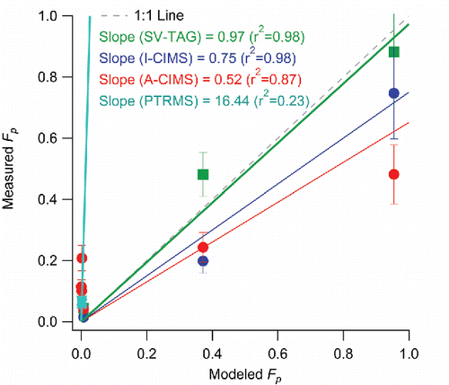
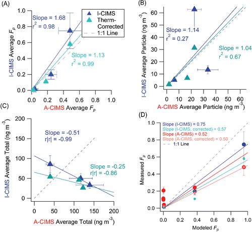
The average measured F_p for the three common species and the entire sampling period are compared in Figure 2a. All three instruments show a consistent trend of increasing F_p with decreasing vapor pressure across the entire range of possible F_p values (0–1), which is consistent with the trend predicted by partitioning theory (Figure 3). These compounds have been found to agree well with the organic absorptive partitioning model in a previous study at a different site using A-CIMS (Yatavelli et al. 2014a). When plotted against the A-CIMS, the average F_p show slopes of 1.86 (r² = 0.99) and 1.68 (r² = 0.98) for SV-TAG and I-CIMS, respectively. The I-CIMS reports consistent F_p values with the A-CIMS within the estimated uncertainties. The SV-TAG measures higher values than the A-CIMS that cannot be explained by the estimated uncertainties, but is within uncertainty of the I-CIMS for two of the three compounds. Note that the estimated uncertainties do not include uncharacterized effects as discussed above. All instruments report gas, particle, and total concentrations of the same order of magnitude, typically of tens to hundreds of ng m⁻³ for the three species. The absolute concentrations measured show varying degrees of agreement and correlation. The SV-TAG and A-CIMS show excellent agreement (slope = 1.03 and r² = 0.97) for the average particle phase concentrations (Figure 2b), while the gas-phase measurements show more scatter, primarily due to a 2.5 times lower pinic acid gas-phase concentration in SV-TAG vs. A-CIMS (Figure 2c). I-CIMS vs. A-CIMS particle phase concentrations are of the same order but show significant scatter (r² = 0.27), while the gas-phase concentrations are much lower in the I-CIMS than in the A-CIMS for the two lower volatility species. For the total concentrations an anti-correlation is observed, which is mainly due to the gas-phase pinic acid measurement. This might be due to the presence of multiple isomers with that elemental formula, which the two instruments measure with different sensitivities. Evidence for this effect will be presented in Section 3.1.5. Thus the study-average comparison shows mixed results: F_p values show high correlation, but there are substantial disagreements in some of the concentrations. In the next 3 sections, we explore the three comparisons at high time resolution (one hour), which is the reporting interval of most of the instruments.

Figure 2. Scatter plots of (a) the average measured F_p (averaging all measurements for each compound), (b) particle-phase concentration, (c) gas-phase concentration, and (d) total concentration over the entire overlap period from SV-TAG and I-CIMS vs. A-CIMS. Each point represents one of the three compounds discussed in Section 3.1. Error bars represent estimated instrumental uncertainties as described in Section 2.5. Regression lines are fixed through the origin and computed using the orthogonal distance regression method (ODR). The A-CIMS was chosen for the x-axis because it is the only instrument that can be compared with all the other instruments (the I-CIMS, SV-TAG, and also the PTRMS). Note that we use r|r| for the I-CIMS/A-CIMS comparison in (d) since r < 0.

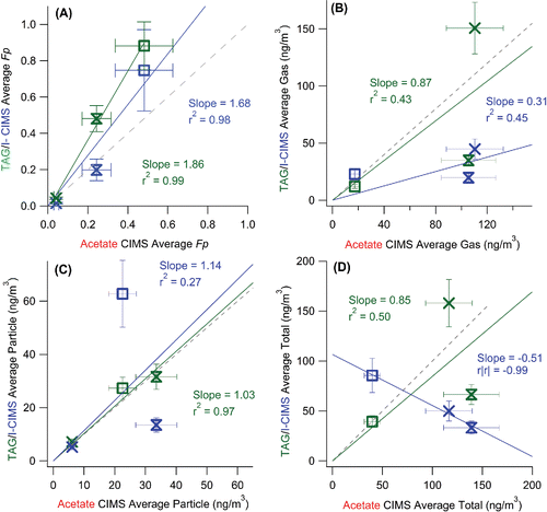
Figure 3. Comparison of average F_p values vs. those modeled using organic absorptive partitioning theory. Regression lines are fixed through the origin (since all instruments performed zero tests and are expected to report zero concentrations when the relevant species are not present) and computed using the orthogonal distance regression method (ODR). See text for more details on modeling.

3.1.2. Detailed comparisons for pinonic acid

All three instruments measured C₁₀H₁₆O₃ (“pinonic acid,” where the quotes indicate some ambiguity on the true species detected, as discussed below). The CIMS instruments identified it via its elemental formula, and the SV-TAG by a match of retention time and mass spectrum with a standard. We note that the CIMS measurements may also include other species of the same elemental composition, and the same applies to other species intercompared and discussed below. There are many possible isomers for this elemental formula, several of which are acids (measurable by the A-CIMS) and other oxidized compounds (potentially measurable by the I-CIMS in addition to pinonic acid and its acid isomers). Pinonic acid is an oxidation product of α−pinene (Szmigielski et al. 2007) and is therefore expected at this field site where α-pinene was abundant.

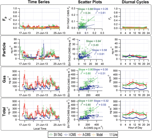
Figure 4 shows the time series, scatter plot, and diurnal cycle of F_p (top), particle phase concentration (second row), gas phase concentration (third row) and total (particle + gas) concentration (bottom). This species was mostly in the gas phase with an F_p below 7% for the diurnal averages, according to all instruments. Some correlation is observed in all comparisons, although with a substantial amount of scatter, with R² in the range 0.34-0.80. For the SV-TAG and A-CIMS 40% of the F_p points are within a factor of two of each other and for the I-CIMS and A-CIMS 26% of the points are within a factor of two of each other, illustrating the degree of scatter. The SV-TAG and A-CIMS show better agreement for both gas and particle concentrations. In contrast, the I-CIMS tends to report lower concentrations than the A-CIMS, albeit with higher correlation than SV-TAG/A-CIMS for the particle concentration. Averaging the individual data points into diurnal cycles results in smooth variations in most cases, with comparison trends similar to those already discussed. All the instruments are consistent with the organic absorptive partitioning model prediction that “pinonic acid” is almost entirely in the gas phase, though none are as low as the model, and all show different diurnal cycles. There is a substantial uncertainty in the model predictions due to large uncertainties in vapor pressures (Bilde et al. 2015) and the assumption of an activity coefficient of one, which could account for some of the model/measurement differences. Partitioning to the aqueous phase is estimated to be negligible for this species with a modeled aqueous phase F_p of 1.4 × 10⁻⁸.

Figure 4. “Pinonic Acid.” Time series (left), scatter plots (center) and diurnal cycles (right) of the measured particle-phase fraction (F_p, top row), and particle phase (2nd row), gas phase (3rd row) and total concentrations (bottom row) for the A-CIMS, I-CIMS, and SV-TAG. Error bars represent estimated instrumental uncertainties as described in Section 2.5. F_p values modeled with absorptive partitioning are also shown in the top row. Regressions lines are fixed through the origin and computed using the orthogonal distance regression method (ODR). The spike in the I-CIMS data is believed to be real, but the reason for it is unclear.

3.1.3. Potential reasons for the observed differences

There are many possible reasons for the disagreements between the instruments beyond the estimated uncertainties. All the reasons are enumerated here, and the most relevant to latter comparisons will be briefly mentioned when each of the subsequent compounds is discussed.

1. Limited signal-to-noise. Individual 1-h data points often display substantial scatter that may be partially due to limited signal-to-noise ratio of the measurements. Some measurement errors may be underestimated for cases with low signal-to-noise. However, in multiple cases systematic differences are observed that are not due to random noise. Similarly, differences beyond the uncertainties are often observed in the diurnal cycles. Thus limited signal-to-noise cannot explain all of the observed differences. Also, in most cases the signals being discussed are fairly large.

2. Inlet and/or instrument adsorption/desorption of gases. We estimate the fraction of gas-phase species penetrating into each instrument without contacting the walls (assuming laminar flow and a gas-phase diffusion coefficient of 5×10⁻⁶ m² s⁻¹,estimated with SPARC for C₅H₁₀O₅ (Hilal et al. 2003, 2007; Krechmer et al. 2015; Knopf et al. 2015) as 10% (39%), 41%, 38%, and 61% for A-CIMS (A-CIMS with shorter inlet, see below), I-CIMS, SV-TAG, and PTR-MS. These estimates neglect the effect of tubing bends as well as surfaces in the instruments themselves, so it appears that there is significant potential for gas/wall interactions to play a role in the measurements. Such effects could lead to reduced concentrations or memory effects, which could differ by instrument. For all instruments lower gas concentrations would be expected due to inlet adsorption, while for the SV-TAG and PTRMS an incomplete capture of gases by the denuders could result in the opposite effect, although these inlet effects are not well understood; e.g., there is much recent evidence for wall loss of semivolatile species to PTFE Teflon walls in chambers (Matsunaga and Ziemann 2010; Zhang et al. 2014a; La et al. 2015; Yeh and Ziemann 2015; Krechmer et al. 2016), but similar effects for PTFE Teflon inlets have not yet been studied in detail. To test for denuder breakthrough in the SV-TAG samples are collected with both a denuder and a filter inline. Any measured signal is assumed to be incomplete capture by the denuder. This is observed to be negligible for all compounds discussed here. To study such inlet effects in the A-CIMS, the instrument was reconfigured for 10 days such that the gas phase inlet was approximately 1/12 of the original length (1/2 m vs. 6 m). No significant difference was observed in F_p (Figure S5), suggesting the lack of a large effect of the PTFE Teflon inlet on gas-phase measurements. However, Krechmer et al. (2016) have reported a significant effect of adsorption for semivolatile gases for the PTFE Teflon inlet plus IMR combination used in both CIMS instruments in this study. This leaves the possibility that a short inlet still had an effect significant enough that a larger discrepancy would not be quantified by the comparison of the two inlet configurations, or that most of the effect is related to the ionization region surfaces. Continuation of studies to characterize the response of each field inlet/instrument source combination to the species of interest is highly recommended.

3. Differences in the particle size ranges of the instruments. All instruments sampled different particle size ranges. Upper size cuts were 2.5, 2, 1, and 2 μm for A-CIMS, I-CIMS, SV-TAG, and PTR-MS, respectively. The lower size cut of the PTR-MS was 70 nm, compared with ∼20 nm for the other instruments. In addition devices with the same nominal size cut can have different detailed transmission curves. Although all instruments were sampling the accumulation mode where most of the organic material was present, the different size ranges may have led to some differences for the particle measurements. Standardization of the size ranges sampled and the size cut devices is recommended for future intercomparisons.

4. Differences in the methods used to quantify instrument backgrounds. While backgrounds and tests were incorporated into the analysis conducted for all instruments to correct for inlet issues, the detailed methods were different for each instrument. The effects are complex and often depend on the specific species. Standardization of background methods, and/or intercomparison of the methods, when possible, are recommended for future intercomparisons.

5. Errors in high-resolution fitting of overlapping ion groups. The CIMS/PTRMS measurements involve extracting the intensity of an individual ion in a group of several overlapping ions. The presence of the overlapping ions increases the uncertainty of the quantification (Cubison and Jimenez 2015). In addition, there may be more ions present in a group than can be unequivocally determined from the data (Stark et al. 2015b). These effects likely differ for each instrument.

6. Differences in the species included in each measurement due to instrument sensitivities (in the absence of thermal decomposition). The CIMS/PTRMS instruments measured the sum of all isomers with the same elemental composition, thus it is possible that the measurements include isomers other than the one targeted. IMS data shown below suggests that different isomers almost certainly play a role in some comparisons. Different species will likely have different time series and F_p, which could result in some of the observed differences. Note that species with the same elemental composition can have C* that differ by several orders-of-magnitude (Krechmer et al. 2015) and that kinetic processes impacting F_p may depend on structural details like functional groups. It is also possible that the CIMS/PTRMS instruments measured the same isomers, but with different relative sensitivities to each isomer, which would result in differences in the total concentration measurement time series, F_p, etc. Ion clustering could result in this type of bias as well, but it is thought to be minor or negligible for the CIMS/PTRMS instruments as used in this study. For the SV-TAG instrument, this type of effect is less likely, since the combination of retention time and mass spectral match generally allows for the separation and identification of different chemical isomers.

7. Differences in negative thermal decomposition (or ion fragmentation) artifacts. A negative artifact is possible for all instruments, in which the species of interest partially decomposes to smaller species. Thermal decomposition of oxygenated species upon heating is a well-known but complex process (Moldoveanu 2009; Canagaratna et al. 2015) and can result in reduced signal levels when the species of interest partially decomposes to smaller fragments. The instruments have significant differences in their thermal desorption profiles (Figure 1). In particular, the SV-TAG exposes the particle-phase compounds to chromatographic analysis and valve transfers involving temperatures higher than needed for purely thermal desorption. The SV-TAG also heats the gas-phase species during analysis, while this is not the case for either CIMS. Because of the GC analysis step, the SV-TAG also subjects the compounds to two heating cycles compared to one for the CIMS. The PTRMS uses heated transfer lines and subjects all gas and particle species to 200°C temperatures. Thus all instruments may suffer from thermal decomposition, although the CIMS instruments have the ability to resolve this effect to some extent. The SV-TAG and PTRMS may be more sensitive to thermal decomposition due to the higher temperatures used, although residence time and surface materials also play a role, so it is not possible to reach firm conclusions. This effect would lead to artificially lower F_p for the CIMS instruments, as these instruments use heat for the particles but not the gases. The use of authentic standards that are exposed to the same desorption processes for calibrations for SV-TAG minimizes the impact of these negative artifacts for the calibrated species, though it remains a possibility that they have some influence. It may also play a role for the many species that are not calibrated for in the SV-TAG. This effect may cancel out for F_p for the TAG and PTRMS since the temperature profiles undergone by gases and particles are similar, but would lead to overall lower species concentrations. Differences in fragmentation of molecular ions of the species of interest could produce a similar difference. Some evidence of partial thermal decomposition during the heating cycles of calibration compounds is shown in Figure S6.

8. Differences in positive thermal decomposition artifacts. A positive artifact is also possible, in which the particle-phase signal of a species is artificially increased due to the decomposition of larger molecules (e.g., oligomers including the species of interest as a monomer, and/or other thermal decomposition products). This would lead to a larger measured F_p than would be expected given the measured species composition and volatility, as has been demonstrated for products of isoprene chemistry at this site by Lopez-Hilfiker et al. (2016)and for a large variety of biogenic products measured at this site by SV-TAG (Isaacman-VanWertz et al. 2016). Some insight into this thermal decomposition issue can be obtained from the CIMS thermograms, as discussed below. As above, differences in ion fragmentation of molecules that produce the species of interest could produce a similar difference. Finally, this effect could also play a role for the gas-phase measurements of SV-TAG and PTR-MS due to the exposure to higher temperatures, although this is less likely than for particle-phase measurements as species such as oligomers are expected to be predominantly in the particle-phase.

3.1.4. Additional evidence for the pinonic acid case

To further investigate the discrepancies mentioned above, two additional layers of data for the CIMS measurements were investigated. Figure 5 shows the high resolution peak fitting used to identify this elemental formula in the A-CIMS and I-CIMS. The peak under study (C₁₀H₁₅O₃⁻) is part of a larger group of peaks, increasing signal uncertainty. However, the peak separation is large enough that the error estimated to arise from peak fitting isonly ∼15%(Cubison and Jimenez 2015), which is significantly smaller than the observed differences between the instruments. The situation for the I-CIMS (Figure 5c) is similar. Cubison and Jimenez (2015) estimated the fitting uncertainties based on computational experiments. It is possible that fitting uncertainties in real measurements are larger, and these should be the subject of additional study (including experiments to better quantify uncertainties).

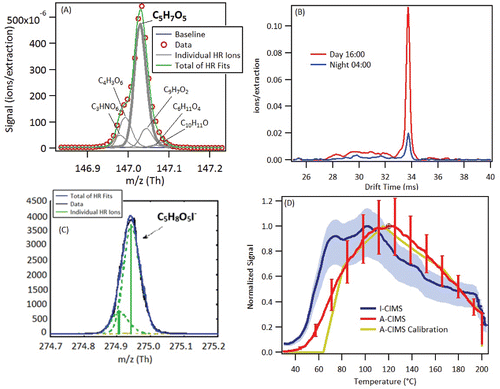
Figure 5. Additional evidence for the formula C₁₀H₁₆O₃ (pinonic acid and isomers, measured in the A-CIMS as C₁₀H₁₅O₃⁻ and in the I-CIMS as C₁₀H₁₆O₃I⁻). (a) High resolution signal fits from the A-CIMS from a one-day averaged mass spectrum. Formula under study is in bold. (b) Signal vs. temperature for the average ambient heating cycle during SOAS from the A-CIMS and the I-CIMS as the FIGAERO filter is slowly heated (see text for details). Averages were taken over the 10 days of the study to encompass a range of days and time of day. Variability (1σ) shown in error bars for A-CIMS and shading for I-CIMS. A calibration thermogram within a mixture of 50 compounds is shown. Calibrations carried out using a mixture of 50 compounds of varying volatility, but the ambient aerosol will have a different composition and also contains substantial fractions of inorganic species that were not present in the calibration mixture. The amount deposited was kept close to ambient amounts. (c) High resolution signal fits from the I-CIMS from a one-day averaged mass spectrum. Formula under study is in bold.

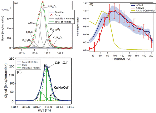
Figure 5b shows average thermal desorption profiles from both CIMS instruments for this elemental composition, which are quite similar. Also shown is an example calibration profile of pinonic acid (acquired with the A-CIMS), conducted by deposition of a known amount of pinonic acid (dissolved in a mixture of different calibration compounds to simulate ambient conditions, see figure caption for details) onto the FIGAERO filter. The calibration compound desorbs from the filter at much lower temperatures (∼60°C), than most of the ambient signal for both CIMS. It is possible that the ambient signal is not dominated by pinonic acid, but either an isomer with a lower vapor pressure (which would cause it to desorb from the filter at higher temperatures), or the breakdown of a larger molecule or oligomer detected at this elemental formula. It is also possible that the difference is due to different matrix effects between the simple calibration mixture and the complex ambient aerosol. However, laboratory testing of different matrix effects has not shown a shift as large as observed here, so this possibility appears unlikely. These complex aspects of the detection process, which will also present themselves in different ways in the other instruments, make it difficult to reach a firm conclusion for the reasons of the observed differences. A summary of the results of the comparison and possible reasons for these differences (Table 2) suggest interference from isomers and thermal decomposition for this species. The instruments do agree that pinonic acid is almost entirely in the gas phase, and these differences are minor for F_p.

Table 2. Summary of key possibilities that can lead to discrepancies in the species intercompared for each instrument. This table is adapted from the list in Section 3.1.3 (number from that list is in parentheses) and includes only possibilities for which data is available to suggest evidence for or against a given hypothesis. The table also includes our best estimate for the impact that each issue would have on F_p, artificially raising (↑) or lowering (↓) the measured value in relation to the true one, or having an unclear effect (?). Shading indicates the most likely causes of error (red) vs. lower probability or impact (yellow) and minor errors (green).

Acid	Mass Spectral Fitting or Match (#5)	Evidence for Multiple Isomers (#6)	Evidence for Thermal Decomposition(#7-8)
A-CIMS
Pinonic Acid	Minor peak, Fp ?	Yes, Fp ↑	Yes, Fp ↑
Pinic Acid	Minor peak, Fp ?	Yes, Fp ?	Yes, Fp ↑
Hydroxy Glutaric Acid	Major peak (minor error)	No	No
Decanoic Acid	Minor peak, Fp?	No evidence for or against	Yes, Fp ↑
I-CIMS
Pinonic Acid	Minor peak, Fp?	Yes, Fp ↑	Yes, Fp ↑
Pinic Acid	Minor peak, Fp ?	Yes, Fp ?	Yes, Fp ↑
Hydroxy Glutaric Acid	Major peak (minor error)	Yes, Fp↓	No
SV-TAG
Pinonic Acid	Good mass spectral match (minor error)	N/A	No evidence for or against
Pinic Acid	Good mass spectral match (minor error)	N/A	No evidence for or against
Hydroxy Glutaric Acid	Good mass spectral match (minor error)	N/A	No evidence for or against
PTRMS
Decanoic Acid	Major peak (minor error)	Yes, Fp ↑	Yes, Fp ↑

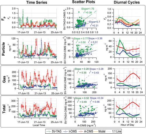
3.1.5. Detailed comparisons for pinic acid

The partitioning values for C₉H₁₄O₄ (“pinic acid”) indicate some level of agreement in the time series, shown in Figure 6, with regression slopes of 0.7 (r² = 0.31) for I-CIMS/A-CIMS and 1.75 (r² = 0.38) for SV-TAG/A-CIMS. For the SV-TAG and A-CIMS 79% of the points are within a factor of two of each other and for the I-CIMS and A-CIMS 52% of the points are within a factor of two of each other, showing some level of agreement. The average diurnal cycles of F_p show a similar temporal trend and magnitude both between the instruments and between the instruments and the absorptive partitioning model, with higher F_p at night and lower during the day. The diurnal trend of the model is more similar to the A-CIMS and I-CIMS (showing a slight offset). The prediction of partitioning to the aqueous phase suggests a median value of 1%, so it is considered negligible. The A-CIMS and SV-TAG instruments show more diurnal variation in the particle and gas concentrations, while the I-CIMS changes less throughout the day. The gas-phase diurnal cycles show an anti-correlation between the SV-TAG and A-CIMS which also manifests itself in the total measurement (with somewhat lesser variation), with the A-CIMS measuring higher gas-phase concentrations than the SV-TAG, and peaking in the afternoon while the SV-TAG peaks at night (and the I-CIMS staying fairly constant throughout the day). These complex differences might be due to some of the reasons discussed in Section 3.1.3. In particular there is evidence that the presence of multiple isomers may be playing an important role, as discussed next.

Figure 6. “Pinic Acid.” Time series (left), scatter plots (center) and diurnal cycles (right) of the measured gas/particle partitioning (F_p top row), particle phase (2nd row), gas phase (3rd row) and total concentration (bottom row) for A-CIMS, I-CIMS, and SV-TAG. Error bars represent instrumental uncertainties as described in Section 2.5. F_p values modeled with absorptive partitioning are also shown in the top row. Regressions lines are fixed through the origin and computed using the orthogonal distance regression method (ODR).

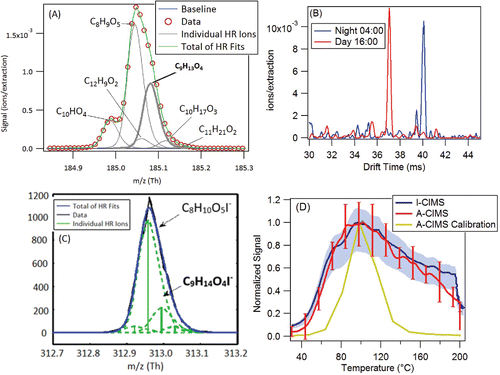
In Figure 7, additional CIMS and ion mobility nitrate IMS-TOF information is shown for this elemental formula. Figure 7a shows that this A-CIMS ion peak (C₉H₁₃O₄⁻) is also part of a larger group of ion peaks, adding an estimated ∼10% uncertainty to the quantification of its area (Cubison and Jimenez 2015), significantly smaller than the observed differences. Figure 7c shows the situation for the I-CIMS, where the ion of interest is ∼1/4 rather than ∼1/2 of the most intense peak in the group. Figure 7b shows two averaged ion mobility spectra for the elemental formula C₉H₁₄O₄⁻, during day and night. One of the isomers is present in the day and absent at night, and the other isomer is present at night and not during the day. Note that the IMS usedNO₃⁻ reagent ions and as such it may detect a different combination of isomers compared to the A-CIMS and I-CIMS. However, it does confirm that there are multiple isomers present and that they have variable relative concentrations during the day/night. In Figure 7c, the average ambient thermal desorption profiles are very similar for A-CIMS and I-CIMS, and show a range of peak desorption temperatures (that show no day/night difference in desorption temperature) with the calibration compound approximately in the middle, in contrast to pinonic acid. The larger desorption profile width in the ambient data is likely due to the presence of several isomers at this molecular formula that have different volatilities, and/or to thermal decomposition of larger molecules, or to different evaporation matrix effects for the calibration vs. ambient aerosol.

Figure 7. Additional evidence for “pinic acid.” (a) High resolution signal fits from the A-CIMS from a one-day averaged mass spectrum. Formula under study is in bold. (b) Two 1 h averaged ion mobility spectra, taken with an ion mobility nitrate chemical ionization mass spectrometer. (c) High resolution signal fits from the I-CIMS from a one-day averaged mass spectrum. Formula under study is in bold. (d) Signal vs. temperature for an averaged ambient heating cycle during SOAS from the A-CIMS and the I-CIMS as the FIGAERO filter is slowly heated (see text for details). Averages were taken over the 10 days of the study to encompass a range of days and time of day. Variation shown in error bars for A-CIMS and shading for I-CIMS. A calibration thermogram with a mixture of 50 compounds is shown. See Figure 4 for more calibration details.

3.1.6. Detailed comparisons for hydroxy glutaric acid

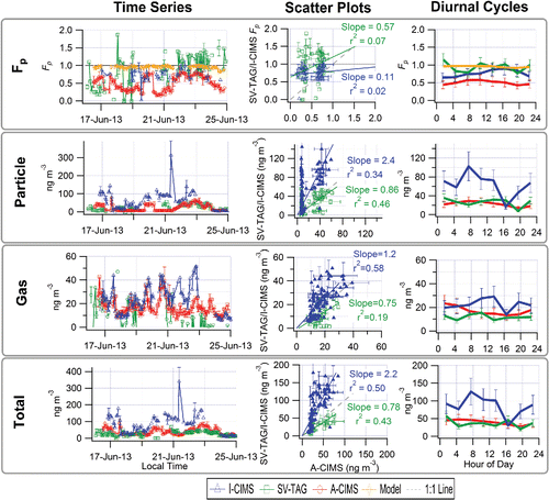
The comparison for C₅H₈O₅ (“hydroxy glutaric acid”), shown in Figure 8, shows similar issues to those of the other two examples. All instruments show two consistent results: (1[1] ) the diurnal cycles show a lack of variation over the course of the day, and (2[2] ) they all measure high particle-phase fractions. For the SV-TAG and A-CIMS 79% of the 1-h datapoints are within a factor of two of each other and for the I-CIMS and A-CIMS 62% of the points are within a factor of two of each other. The organic absorptive partitioning model predicts high partitioning values that do not vary throughout the day as well. The median prediction of partitioning to the aqueous phase is 8%. Thus partitioning is likely to be dominated by the organic phase, although there is some uncertainty in this conclusion given the uncertainty in species thermodynamic properties. The diurnal trend for the organic vs. water partitioning models is very similar (Figure S7) as trends of temperature and aerosol liquid water content are strongly correlated, so the two mechanisms cannot be differentiated based on measured diurnal cycles. It should be noted here that none of the traces from either instrument shows a correlation with inorganics measured at the site. The gas phase shows more consistent concentrations among the three instruments, while the I-CIMS reports higher particle concentrations.

Figure 8. “Hydroxy Glutaric Acid.” Time series (left), scatter plots (center) and diurnal cycles (right) of the measured gas/particle partitioning (F_p, top row), particle phase (2nd row), gas phase (3rd row), and total concentration (bottom row) for A-CIMS, I-CIMS, and SV-TAG. Error bars represent instrumental uncertainties as described in Section 2.5. F_p values modeled with absorptive partitioning are also shown in the top row. Regressions lines are fixed through the origin and computed using the orthogonal distance regression method (ODR).

The high resolution mass spectral fitting for this elemental formula (Figure 9a) shows thatC₅H₇O₅⁻ is the main peak at m/z 147 for A-CIMS, making the peak-fitting uncertainty a very small source of error (<1%) in the quantification. The situation for the I-CIMS (Figure 9c) is similar. The IMS spectra, shown in Figure 9b, show only one isomer at this elemental formula. All of the A-CIMS thermal desorption profiles, shown in Figure 9c, also closely match the calibration compound profile, suggesting that other isomers at different volatilities or the thermal decomposition of other compounds are not interfering with this signal for the A-CIMS. This still leaves the possibility that the compound itself is partially thermally decomposing and is therefore under-measured when heat is used in the measurement. The I-CIMS thermograms, however, show clear evidence of an interfering isomer at lower temperatures.

Figure 9. Additional evidence for the formula C₅H₈O₅ (hydroxy glutaric acid and isomers). (a) High resolution signal fits from the A-CIMS from a one-day averaged mass spectrum. Formula under study is in bold. (b) Two 1 h averaged ion mobility spectra, taken with an ion mobility nitrate chemical ionization mass spectrometer. (c) High resolution signal fits from the I-CIMS from a one-day averaged mass spectrum. Formula under study is in bold. (d) Signal vs. temperature for an averaged ambient heating cycle during SOAS from the A-CIMS and the I-CIMS as the FIGAERO filter is slowly heated (see text for details). Averages taken over the 10 days of the study to encompass a range of days and time of day. Variation shown in error bars for A-CIMS and blue shading for I-CIMS. A calibration thermogram with a mixture of 50 compounds is shown. See Figure 4 for more calibration details.

3.1.7. Approximate correction for isomers and thermal decomposition in both CIMS

A correction was made for both CIMS using the information provided in the thermal desorption profiles. The particle-phase signal was adjusted to match the percentage of the signal believed to be from the compound of interest (based on the calibrations). The total concentration and F_p values were then recalculated using the new particle-phase concentrations. The results of this procedure are shown in Figure 10. When this correction is implemented the agreement of the I-CIMS and A-CIMS is improved, although agreement with the organic absorptive partitioning model is degraded. Thus while these effects likely explain some of the differences between the A-CIMS and I-CIMS, they do not explain the differences between measurement and model. These differences can also be due to model uncertainties, at least in part. No such correction can be performed for the SV-TAG instrument as no thermograms are recorded from the initial particle thermal desorption. SV-TAG peak identification and gas chromatographic identification information is shown in Figure S8.

Figure 10. Results of correcting the campaign-average comparison of A-CIMS and I-CIMS using the estimated signal from isomers and thermal decomposition based on the FIGAERO thermograms. Panels show F_p (a), particle phase signal (b), and total signal (c). Also shown is the corrected average F_p vs. organic absorptive partitioning model (d).

3.2. Comparison of A-CIMS and PTRMS

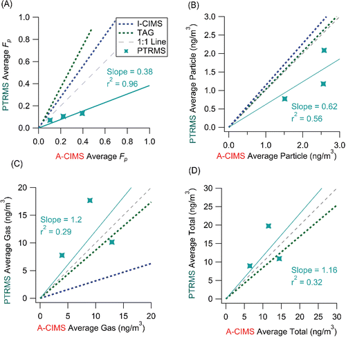
For the comparison between A-CIMS and PTRMS, 3 elemental formulas were chosen based on a match of the elemental formulas assigned to high-resolution peaks in the mass spectra of both instruments. Alkanoic acids (C_XH_2YO₂) are compounds for which there are very few possible isomers with the same elemental formula but different functional group composition, due to their low double bond equivalency (DBE) of one. The compounds vary in their level of agreement. The comparison of the averaged F_p values for each of the species is shown as a scatter plot in Figure 11a. F_p measured by the PTRMS are, on average, about half of the A-CIMS values (slope = 0.38, r² = 0.96). Concentrations are of the same order. The largest difference is observed for the particle-phase concentrations (Figure 11b), as the PTRMS consistently measured lower values, while there is more similarity in the gas-phase and total measurements (Figure 11c and d). The possible reasons for these differences are the same ones discussed in Section 3.1.3. The heated lines (200°C) used in the PTRMS inlet system expose all compounds to high temperatures and could cause some compounds to thermally decompose or be produced by thermal decomposition of larger molecules. By comparison, the A-CIMS only exposes the compounds to the temperature needed to evaporate them from the FIGAERO filter, and the bulk of the measured compounds in this study desorb in the range 70–120°C. However, since both the gas and aerosol use the heated transfer lines in the PTRMS, decomposition may affect them in the same way, and should not lead to a preferential low bias for the particle phase. In addition, the two instruments could be measuring isomers with different functional groups, and thus different vapor pressures and partitioning fractions. Given that most of the A-CIMS compounds measured are alkanoic acids, there are only a few other possible isomers for the PTRMS. One is a hydroxycarbonyl instead of a carboxylic acid group, but according to structure-activity relationships (Pankow and Asher 2008) that would not change the estimated vapor pressure of the molecule by a substantial amount. The F_p values show poor agreement with model values (Figure 3), with substantially larger measurement values (consistent with their C* values shown in Figure S9). This may be due to thermal decomposition of larger molecules into the measured molecules, or to the measurement of different isomers as previously discussed. Previous studies (Yatavelli et al. 2014b) have also observed this measurement of much higher F_p values compared to the organic absorptive partitioning model for alkanoic acids at low carbon numbers in a previous study as well as during SOAS (Figure S10). There is some evidence for this effect in the thermal desorption profiles discussed later.

Figure 11. Scatter plots of the average measured F_p for PTRMS vs. A-CIMS. Each point is an average of all measurements for each compound for (a) F_p (b) particle-phase concentration, (c) gas-phase concentration, and (d) total concentration over the entire measurement overlap period from PTRMS vs. A-CIMS. Error bars represent estimated instrumental uncertainties as described in Section 2.5. Regressions lines are fixed through the origin and computed using the orthogonal distance regression method (ODR). Regression lines for the SV-TAG and I-CIMS vs. A-CIMS are shown as dotted lines for reference.

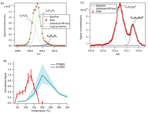
An example time series of F_p along with gas and particle phase concentrations can be found in Figure 12 for “decanoic acid.” The partitioning values agree on order of magnitude but not in diurnal trend, and both measurements are much higher than the modeled organic partitioning values. As discussed above, for the average data for all compounds, the largest difference in concentration is observed for the particle phase, which is lower in the PTRMS than in the A-CIMS. The gas-phase concentrations are more similar, although neither are well correlated. Figure 13a shows the average high-resolution fits for the A-CIMS. Decanoic acid is a small signal at this one, but it is well-separated at the rightmost end of the ion group, about 2.5 half-widths to the right, and the estimated intensity error due to fitting is small. The high-resolution fits for the PTRMS are shown in 13c, and while the main peak is not completely fit the Decanoic acid peak is well separated and well fit. The thermal desorption profiles for the A-CIMS and the PTRMS are shown in Figure 13b. For the thermograms, the A-CIMS shows lower peak desorption temperatures (∼125°C), while the PTRMS shows much higher peak desorption temperatures (∼200°C). There is no thermogram data from calibrations for either instrument, but similar compounds tested in previous work suggest that a compound of this volatility desorb early for the A-CIMS (under 100°C). This suggests that the particle phase signal from both instruments may be at least partially due to thermal decomposition of larger molecules, as discussed above.

Figure 12. Time series (left), scatter plot (center), and diurnal cycle (right) of the measured gas/particle partitioning (F_p), particle phase, gas phase, and total concentration for C₁₀H₂₀O₂ (“decanoic acid”) for the A-CIMS and PTRMS. The C* and ΔH_vap used for the absorptive partitioning model are from Nannoolal et al. (2008) and Chattopadhyay and Ziemann (2005), respectively. Error bars represent estimated instrumental uncertainties as described in Section 2.5. Regressions lines are fixed through the origin and computed using the orthogonal distance regression method (ODR).

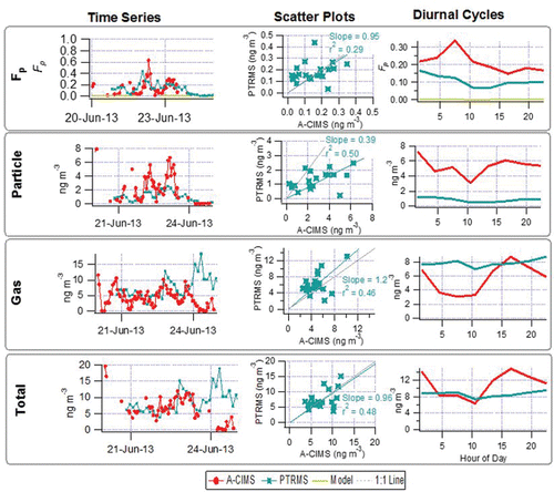
Figure 13. Additional evidence for C₁₀H₂₀O₂. (a) High-resolution peak for the A-CIMS. (b) Average particle-phase thermograms from the A-CIMS, showing field data vs. filter temperature as the FIGAERO filter is slowly heated (see text for details). PTRMS signal vs. temperature as the I-CTD cell is heated is shown. No calibration is available for this compound. (c) High-resolution peak fit for the PTRMS.

4. Conclusions

We have presented the first intercomparison of in-situ near real-time measurements of gas/particle partitioning, a very recently developed capability. We use measurements from the SOAS field campaign in the southeastern United States in the summer of 2013. Although the individual time series of partitioning fractions show a substantial amount of scatter, the three acids compared between the A-CIMS, I-CIMS, and the SV-TAG span the range of possible F_p values and show better agreement when averaged into campaign-long averages. They also follow the trend expected from the organic absorptive partitioning model, with F_p increasing with decreasing species volatility, while partitioning to the aqueous phase is shown to have little/no effect in these cases. The fourth instrument, the PTRMS, showed the same general trend but overall lower aerosol partitioning values than the A-CIMS, with both instruments measuring much higher partitioning values than predicted by the organic absorptive partitioning model for those species.

The intercomparison exercise shows agreement of the average trends and agreement of F_p values often within a factor of 2, where the model values can have substantial uncertainties due to the uncertain vapor pressures. It is unclear whether the model/measurement differences are due to instrumental uncertainty or uncertainty in the model estimation, and it is likely a combination of the two. Better agreement in the measurements is needed before stronger conclusions can be made. Thus there is promise for this new measurement capability, as well as more confidence in the measurement of low vs. high particle-phase fractions. However multiple discrepancies are observed that lie beyond the estimated instrument uncertainties. We suggest that the observed discrepancies could be due to at least eight different effects: (1[1] ) Underestimation of measurement errors under low signal-to-noise conditions; (2[2] ) inlet and/or instrument adsorption/desorption of gases; (3[3] ) differences in particle size ranges sampled; (4[4] ) differences in the methods used to quantify instrument backgrounds; (5[5] ) errors in high-resolution fitting of overlapping ion groups; (6[6] ) differences in the isomers included in each measurement due to different instrument sensitivities; and differences in (7) negative or (8) positive thermal decomposition (or ion fragmentation) artifacts. The available data is insufficient to conclusively identify the reasons for the discrepancies, but evidence from inlet tests with the A-CIMS, thermal desorption profiles of CIMS and PTRMS, laboratory decomposition studies, and IMS-TOF spectra suggests effects 6–8 as playing an important role. Some of the other effects 1–5 may also contribute in some cases. When positive thermal decomposition artifacts are approximately corrected for the agreement between the instruments improves. These comparisons do not clearly indicate that one instrument is performing “better” or “worse” than the others, and further studies are needed to clarify the remaining disagreements.

We recommend performing additional laboratory and field calibrations and experiments aiming to isolate factors 1–8 (or other possible effects not listed here) for each of the instruments. We also recommend additional laboratory and field intercomparisons. It is worth noting that several of the instruments discussed here have been improved since the SOAS 2013 data was collected. For example, the FIGAERO inlet has been modified to improve the heating and cooling apparatus and introduce more reliable background measurements. The SV-TAG has been improved to reduce the noise in the data and lower the error associated with measurement. Our results show the importance and value of using all available data from CIMS and PTRMS instruments (e.g., HR fits, thermograms). Finally, there is a pressing need for separation techniques (such as the IMS-TOF or GC-CIMS) that can be interfaced to the CIMS instruments to allow better separation of structural isomers, and a need to better understand the role of thermal decomposition in all of these instruments as it related to the measurement of gas/particle partitioning.

Acknowledgments

We are grateful to Annmarie Carlton, Karsten Baumann, and Eric Edgerton for their organization of the Centreville Supersite. We thank Julie Phillips of JILA for writing and editing support.

Funding

This research was partially supported by NSF AGS-1243354 and AGS-1360834, DOE (BER/ASR) DE-SC0011105 and DE-SC0016559, DOE SBIR DE-SC0011218, and NOAA NA13OAR4310063. DOE SBIR award DE-SC0004577 supported the development of the FIGAERO-CIMS instrument. SLT and JEK are grateful for CIRES Graduate Fellowships. JEK acknowledges an EPA STAR Graduate Fellowship (FP-91770901-0). EPA has not reviewed this manuscript and no endorsement should be inferred. GIV was supported by NSF Graduate Research Fellowship (#DGE 1106400), and the SV-TAG measurements and the UCB/Aerosol Dynamics team were funded by NSF Atmospheric Chemistry Program #1250569.

ORCID

Jordan E. Krechmer http://orcid.org/0000-0003-3642-0659

Douglas R. Worsnop http://orcid.org/0000-0002-8928-8017

Jose L. Jimenez http://orcid.org/0000-0001-6203-1847

References

- Aljawhary, D., Lee, A. K. Y., and Abbatt, J. P. D. (2013). High-Resolution Chemical Ionization Mass Spectrometry (ToF-CIMS): Application to Study SOA Composition and Processing. Atmos. Meas. Tech., 6:3211–3224, doi:10.5194/amt-6-3211-2013
- Andrews, D. U., Heazlewood, B. R., Maccarone, A. T., Conroy, T., Payne, R. J., Jordan, M. J. T., and Kable, S. H. (2012). Photo-Tautomerization of Acetaldehyde to Vinyl alcohol: A Potential Route to Tropospheric Acids. Science, 337:1203–1206, doi:10.1126/science.1220712
- Bertram, T. H., Kimmel, J. R., Crisp, T. A., Ryder, O. S., Yatavelli, R. L. N., Thornton, J. A., Cubison, M. J., Gonin, M., and Worsnop, D. R. (2011). A Field-Deployable, Chemical Ionization Time-of-Flight Mass Spectrometer. Atmos. Meas. Tech., 4:1471–1479, doi:10.5194/amt-4-1471-2011.
- Bilde, M., Barsanti, K., Booth, M., Cappa, C. D., Donahue, N. M., Emanuelsson, E. U., McFiggans, G., Krieger, U. K., Marcolli, C., Topping, D., Ziemann, P., Barley, M., Clegg, S., Dennis-Smither, B., Hallquist, M., Hallquist, Å. M., Khlystov, A., Kulmala, M., Mogensen, D., Percival, C. J., Pope, F., Reid, J. P., Ribeiro da Silva, M. A. V., Rosenoern, T., Salo, K., Soonsin, V. P., Yli-Juuti, T., Prisle, N. L., Pagels, J., Rarey, J., Zardini, A. A., and Riipinen, I. (2015). Saturation Vapor Pressures and Transition Enthalpies of Low-Volatility Organic Molecules of Atmospheric Relevance: From Dicarboxylic Acids to Complex Mixtures. Chem. Rev.,:150501082359009, doi:10.1021/cr5005502
- Bilde, M., and Pandis, S. N. (2001). Evaporation Rates and Vapor Pressures of Individual Aerosol Species Formed in the Atmospheric Oxidation of α- and β-Pinene. Environ. Sci. Technol., 35:3344–3349, doi:10.1021/es001946b.
- Canagaratna, M. R., Jimenez, J. L., Kroll, J. H., Chen, Q., Kessler, S. H., Massoli, P., Hildebrandt Ruiz, L., Fortner, E., Williams, L. R., Wilson, K. R., Surratt, J. D., Donahue, N. M., Jayne, J. T., and Worsnop, D. R. (2015). Elemental Ratio Measurements of Organic Compounds Using Aerosol Mass Spectrometry: Characterization, Improved Calibration, and Implications. Atmos. Chem. Phys., 15:253–272, doi:10.5194/acp-15-253-2015
- Carlton, A. M., de Gouw, J., Jimenez, J. L., Ambrose, J. L., Brown, S., Baker, K. R., Brock, C. A., Cohen, R. C., Edgerton, S., Farkas, C., Farmer, D., Goldstein, A. H., Gratz, L., Guenther, A., Hunt, S., Jaeglé, L., Jaffe, D. A., Mak, J., McClure, C., Nenes, A., Nguyen, T. K. V., Pierce, J. R., Selin, N., Shah, V., Shaw, S., Shepson, P. B., Song, S., Stutz, J., Surratt, J., Turpin, B. J., Warneke, C., Washenfelder, R. A., Wennberg, P. O., and Zhou, X. (2016). Atmosphere Studies (SAS): Coordinated Investigation and Discovery to Answer Critical Questions About Fundamental Atmospheric Processes. Bull. Am. Met. Soc, submitted.
- Chattopadhyay, S., and Ziemann, P. J. (2005). Vapor Pressures of Substituted and Unsubstituted Monocarboxylic and Dicarboxylic Acids Measured Using an Improved Thermal Desorption Particle Beam Mass Spectrometry Method. Aerosol Sci. Technol., 39:1085–1100, doi:10.1080/02786820500421547
- Chebbi, A., and Carlier, P. (1996). Carboxylic Acids in the Troposphere, Occurrence, Sources, and Sinks: A Review. Atmos. Environ., 30:4233–4249, doi:10.1016/1352-2310(96)00102-1
- Compernolle, S., and Müller, J.-F. (2013). Henry's Law Constants of Diacids and Hydroxypolyacids: Recommended Values. Atmos. Chem. Phys., 13:25125–25156, doi:10.5194/acpd-13-25125-2013
- Cubison, M. J., and Jimenez, J. L. (2015). Statistical Precision of the Intensities Retrieved from Constrained Fitting of Overlapping Peaks in High-Resolution Mass Spectra. Atmos. Meas. Tech., 8:2333–2345, doi:10.5194/amt-8-2333-2015
- Decarlo, P. F., Kimmel, J. R., Trimborn, A., Northway, M. J., Jayne, J. T., Aiken, A. C., Gonin, M., Fuhrer, K., Horvath, T., Docherty, K. S., Worsnop, D. R., and Jimenez, J. L. (2006). Field-Deployable, High-Resolution, Time-of-Flight Aerosol Mass Spectrometer. Anal. Chem., 78:8281–8289, doi:10.1029/2001JD001213.Analytical.
- de Gouw, J. A. (2005). Budget of Organic Carbon in a Polluted Atmosphere: Results from the New England Air Quality Study in 2002. J. Geophys. Res., 110:D16305, doi:10.1029/2004JD005623
- de Gouw, J., and Jimenez, J. L. (2009). Organic Aerosols in the Earth's Atmosphere. Environ. Sci. Technol., 43:7614–7618, doi:10.1021/Es9006004
- Donahue, N. M., Robinson, A. L., Stanier, C. O., and Pandis, S. N. (2006). Coupled Partitioning, Dilution, and Chemical Aging of Semivolatile Organics. Environ. Sci. Technol., 40:2635–643.[online] Available from: http://www.ncbi.nlm.nih.gov/pubmed/16683603(Accessed 21 January 2014).
- Dzepina, K., Volkamer, R. M., Madronich, S., Tulet, P., Ulbrich, I. M., Zhang, Q., Cappa, C. D., Ziemann, P. J., and Jimenez, J. L. (2009). Evaluation of Recently-Proposed Secondary Organic Aerosol Models for a Case Study in Mexico City. Atmos. Chem. Phys.,9:5681–5709, doi:10.5194/acp-9-5681-2009
- Eiceman, G. A., and Karpas, Z. (2010). Ion Mobility Spectrometry, Second Edition. Taylor & Francis, New York, NY.
- Ervens, B. (2015). Modeling the Processing of Aerosol and Trace Gases in Clouds and Fogs. Chem. Rev., 115(10):4157–4198.
- Faulhaber, A. E., Thomas, B. M., Jimenez, J. L., Jayne, J. T., Worsnop, D. R., and Ziemann, P. J. (2009). Characterization of a Thermodenuder-Particle Beam Mass Spectrometer System for the Study of Organic Aerosol Volatility and Composition. Atmos. Meas. Tech., 2(1):15–31.
- Goldstein, A. H., and Galbally, I. E. (2007). Known and Unexplored Organic Constituents in the Earth's Atmosphere. Environ. Sci. Technol., 41:1515–1521[online] Available from: http://pubs.acs.org/doi/abs/10.1021/es072476p (Accessed 26 December 2013).
- Guo, H., Xu, L., Bougiatioti, A., Cerully, K. M., Capps, S. L., Hite, J. R., Carlton, A. G., Lee, S.-H., Bergin, M. H., Ng, N. L., Nenes, A., and Weber, R. J. (2015). Fine-Particle Water and pH in the Southeastern United States. Atmos. Chem. Phys., 15:5211–5228, doi:10.5194/acp-15-5211-2015
- Hallquist, M., Wenger, J. C., Baltensperger, U., Rudich, Y., Simpson, D., Claeys, M., Dommen, J., Donahue, N. M., George, C., Goldstein, A. H., Hamilton, J. F., Herrmann, H., Hoffmann, T., Iinuma, Y., Jang, M., Jenkin, M. E., Jimenez, J. L., Kiendler-Scharr, A., Maenhaut, W., McFiggans, G., Mentel, T. F., Monod, A., Prévôt, A. S. H., Seinfeld, J. H., Surratt, J. D., Szmigielski, R., and Wildt, J. (2009). The Formation, Properties and Impact of Secondary Organic Aerosol: Current and Emerging Issues. Atmos. Chem. Phys., 9:5155–5236, doi:10.5194/acp-9-5155-2009.
- Hilal, S. H. H., Karickhoff, S. W. W., and Carreira, L. A. A. (2003). Prediction of the Vapor Pressure Boiling Point, Heat of Vaporization and Diffusion Coefficient of Organic Compounds. QSAR Comb. Sci.,22(6):565–574, doi:10.1002/qsar.200330812
- Hilal, S. H., Saravanaraj, A. N., Whiteside, T., and Carreira, L. A. (2007). Calculating physical properties of organic compounds for environmental modeling from molecular structure. J. Comput. Aided. Mol. Des., 21(12):693–708, doi:10.1007/s10822-007-9134-y
- Holzinger, R. (2015). PTRwid: A New Widget-Tool for Processing PTR-TOF-MS Data. Atmos. Meas. Tech. Discuss., 8:1629–1669, doi:10.5194/amtd-8-1629-2015.
- Holzinger, R., Williams, J., Herrmann, F., Lelieveld, J., Donahue, N. M., and Röckmann, T. (2010). Aerosol analysis using a Thermal-Desorption Proton-Transfer-Reaction Mass Spectrometer (TD-PTR-MS): A New Approach to Study Processing of Organic Aerosols. Atmos. Chem. Phys., 10:2257–2267, doi:10.5194/acp-10-2257-2010.
- Hu, W. W., Campuzano-Jost, P., Palm, B. B., Day, D. A., Ortega, A. M., Hayes, P. L., Krechmer, J. E., Chen, Q., Kuwata, M., Liu, Y. J., de Sá, S. S., Martin, S. T., Hu, M., Budisulistiorini, S. H., Riva, M., Surratt, J. D., St. Clair, J. M., Isaacman-Van Wertz, G., Yee, L. D., Goldstein, A. H., Carbone, S., Artaxo, P., de Gouw, J. A., Koss, A., Wisthaler, A., Mikoviny, T., Karl, T., Kaser, L., Jud, W., Hansel, A., Docherty, K. S., Robinson, N. H., Coe, H., Allan, J. D., Canagaratna, M. R., Paulot, F., Jimenez, J. L., McKinney, K., Martin, S. T., Hu, M., Budisulistiorini, S. H., Riva, M., Surratt, J. D., St. Clair, J. M., Isaacman-Van Wertz, G., Yee, L. D., Goldstein, A. H., Carbone, S., Brito, J., Artaxo, P., de Gouw, J. A., Koss, A., Wisthaler, A., Mikoviny, T., Karl, T., Kaser, L., Jud, W., Hansel, A., Docherty, K. S., Alexander, M. L., Robinson, N. H., Coe, H., Allan, J. D., Canagaratna, M. R., Paulot, F., and Jimenez, J. L. (2015). Characterization of a Real-Time Tracer for Isoprene Epoxydiols-derived Secondary Organic Aerosol (IEPOX-SOA) from aerosol mass spectrometer measurements. Atmos. Chem. Phys., 15:11223–11276, doi:10.5194/acpd-15-11223-2015.
- Huey, L. G., Hanson, D. R., and Howard, C. J. (1995). Reactions of SF6- and I- with Atmospheric Trace Gases. J. Phys. Chem., 99:5001–5008, doi:10.1021/j100014a021
- Isaacman, G., Kreisberg, N. M., Yee, L. D., Worton, D. R., Chan, A. W. H., Moss, J. A., Hering, S. V., and Goldstein, A. H. (2014). Online Derivatization for Hourly Measurements of Gas-and Particle-Phase Semi-Volatile Oxygenated Organic Compounds by Thermal Desorption Aerosol Gas Chromatography (SV-TAG). Atmos. Meas. Tech.,7:4417–4429, doi:10.5194/amt-7-4417-2014.
- Isaacman-VanWertz, G., Yee, L. D., Kreisberg, N. M., Wernis, R., Moss, J. A., Hering, S. V, de Sa, S. S., Martin, S. T., Alexander, L. M., Palm, B. B., Hu, W., Campuzano-Jost, P., Day, D. A., Jimenez, J. L., Riva, M., Surratt, J. D., Viegas, J., Manzi, A., Edgerton, E. S., Baumann, K., Souza, R., Artaxo, P., and Goldstein, A. H. (2016). Ambient Gas-Particle Partitioning of Tracers for Biogenic Oxidation. Environ. Sci. Technol., 50(18):9952–9962.
- IPCC. (2013). Climate Change 2013: The Physical Science Basis. Contribution of Working Group I to the Fifth Assessment Report of the Intergovernmental Panel on Climate Change. Stocker, T.F., D. Qin, G.-K. Plattner, M. Tignor, S.K. Allen, J. Boschung, A. Nauels, Y. Xia, V. Bex and P.M. Midgley. (eds.). Cambridge University Press, Cambridge, United Kingdom and New York, NY. 1535 pp.
- Jimenez, J. L., Canagaratna, M. R., Donahue, N. M., Prevot, a S. H., Zhang, Q., Kroll, J. H., DeCarlo, P. F., Allan, J. D., Coe, H., Ng, N. L., Aiken, A C., Docherty, K. S., Ulbrich, I. M., Grieshop, A. P., Robinson, A. L., Duplissy, J., Smith, J. D., Wilson, K. R., Lanz, V. A., Hueglin, C., Sun, Y. L., Tian, J., Laaksonen, A., Raatikainen, T., Rautiainen, J., Vaattovaara, P., Ehn, M., Kulmala, M., Tomlinson, J. M., Collins, D. R., Cubison, M. J., Dunlea, E. J., Huffman, J. A., Onasch, T. B., Alfarra, M. R., Williams, P. I., Bower, K., Kondo, Y., Schneider, J., Drewnick, F., Borrmann, S., Weimer, S., Demerjian, K., Salcedo, D., Cottrell, L., Griffin, R., Takami, A., Miyoshi, T., Hatakeyama, S., Shimono, A., Sun, J. Y., Zhang, Y. M., Dzepina, K., Kimmel, J. R., Sueper, D., Jayne, J. T., Herndon, S. C., Trimborn, A. M., Williams, L. R., Wood, E. C., Middlebrook, A. M., Kolb, C. E., Baltensperger, U., and Worsnop, D. R. (2009). Evolution of Organic Aerosols in the Atmosphere. Science, 326:1525–1529, doi:10.1126/science.1180353
- Kanakidou, M., Seinfeld, J. H., Pandis, S. N., Barnes, I., Dentener, F. J., Facchini, M. C., Van Dingenen, R., Ervens, B., Nenes, A., Nielsen, C. J., Swietlicki, E., Putaud, J. P., Balkanski, Y., Fuzzi, S., Horth, J., Moortgat, G. K., Winterhalter, R., Myhre, C. E. L., Tsigaridis, K., Vignati, E., Stephanou, E. G., and Wilson, J. (2005). Organic Aerosol and Global Climate Modelling: A Review. Atmos. Chem. Phys.,5:1053–1123, doi:10.5194/acp-5-1053-2005.
- Kaplan, K., Graf, S., Tanner, C., Gonin, M., Fuhrer, K., Knochenmuss, R., Dwivedi, P., and Hill, H. H. (2010). Resistive Glass IM-TOFMS. Anal. Chem., 82:9336–9343, doi:10.1021/ac1017259
- Knopf, D. A., Pöschl, U., and Shiraiwa, M. (2015). Radial Diffusion and Penetration of Gas Molecules and Aerosol Particles through Laminar Flow Reactors, Denuders, and Sampling Tubes. Anal. Chem., 87(7):3746–3754.
- Krechmer, J. E., Coggon, M. M., Massoli, P., Nguyen, T. B., Crounse, J. D., Hu, W., Day, D. A., Tyndall, G. S., Henze, D. K., Rivera-Rios, J. C., Nowak, J. B., Kimmel, J. R., Mauldin, R. L., Stark, H., Jayne, J. T., Sipilä, M., Junninen, H., St Clair, J. M., Zhang, X., Feiner, P. A., Zhang, L., Miller, D. O., Brune, W. H., Keutsch, F. N., Wennberg, P. O., Seinfeld, J. H., Worsnop, D. R., Jimenez, J. L., Canagaratna, M. R., Clair, J. M., St. Zhang, X., Feiner, P. A., Zhang, L., Miller, D. O., Brune, W. H., Keutsch, F. N., Wennberg, P. O., Seinfeld, J. H., Worsnop, D. R., Canagaratna, M. R., and Jimenez, J. L. (2015). Formation of Low Volatility Organic Compounds and Secondary Organic Aerosol from Isoprene Hydroxyhydroperoxide Low-NO Oxidation. Environ. Sci. Technol., 49:10330–10339, doi:10.1021/acs.est.5b02031
- Krechmer, J. E., Groessl, M., Zhang, X., Junninen, H., Massoli, P., Lambe, A. T., Kimmel, J. R., Cubison, M. J., Graf, S., Lin, Y.-H., Budisulistiorini, S. H., Zhang, H., Surratt, J. D., Knochenmuss, R., Jayne, J. T., Worsnop, D. R., Jimenez, J.-L., and Canagaratna, M. R. (2016). Ion Mobility Spectrometry–Mass Spectrometry (IMS–MS) for on-and Offline Analysis of Atmospheric Gas and Aerosol Species. Atmos. Meas. Tech., 9(7):3245–3262, doi:10.5194/amt-9-3245-2016.
- Krechmer, J. E., Pagonis, D., Ziemann, P. J., and Jimenez, J. L. (2016). Quantification of Gas-Wall Partitioning in Teflon Environmental Chambers Using Rapid Bursts of Low-Volatility Oxidized Species Generated in-Situ. Prep., 50(11):5757–5765.
- La, Y. S., Camredon, M., Ziemann, P. J., Valorso, R., Matsunaga, A., Lannuque, V., Lee-Taylor, J., Hodzic, A., Madronich, S., and Aumont, B. (2015). Impact of Chamber Wall Loss of Gaseous Organic Compounds on Secondary Organic Aerosol Formation: Explicit Modeling of SOA Formation From Alkane and Alkene Oxidation. Atmos. Chem. Phys. Discuss., 15:23893–23930, doi:10.5194/acpd-15-23893-2015.
- Lee, B. H., Lopez-Hilfiker, F. D., Mohr, C., Kurtén, T., Worsnop, D. R., and Thornton, J. A. (2014). An Iodide-Adduct High-Resolution Time-of-Flight Chemical-Ionization Mass Spectrometer: Application to Atmospheric Inorganic and Organic Compounds. Environ. Sci. Technol., 48:6309–6317, doi:10.1021/es500362a
- Lim, Y. B., Tan, Y., Perri, M. J., Seitzinger, S. P., and Turpin, B. J. (2010). Aqueous Chemistry and Its Role in Secondary Organic Aerosol (SOA) Formation. Atmos. Chem. Phys.,10:10521–10539, doi:10.5194/acp-10-10521-2010.
- Lopez-Hilfiker, C., Mohr, E.L., D'Ambro, A., Lutz, T.P., Riedel, C.J., Gaston, S., Iyer, Z., Zhang, A., Gold, J.D., Surratt, B.H., Lee, T., Kurten, W.W., Hu, J.L., Jimenez, M., and Hallquist, J. A. T. (2016). Molecular Composition and Volatility of Organic Aerosol Formed in a Polluted Isoprene-Rich Region. Environ. Sci. Technol., 50(5):2200–2209.
- Lopez-Hilfiker, F. D., Mohr, C., Ehn, M., Rubach, F., Kleist, E., Wildt, J., Mentel, T. F., Carrasquillo, A. J., Daumit, K. E., Hunter, J. F., Kroll, J. H., Worsnop, D. R., and Thornton, J. A. (2015). Phase Partitioning and Volatility of Secondary Organic Aerosol Components Formed From α-Pinene Ozonolysis and OH Oxidation: the Importance of Accretion Products and Other Low Volatility Compounds. Atmos. Chem. Phys.,15:7765–7776, doi:10.5194/acp-15-7765-2015.
- Lopez-Hilfiker, F. D., Mohr, C., Ehn, M., Rubach, F., Kleist, E., Wildt, J., Mentel, T. F., Lutz, A., Hallquist, M., Worsnop, D., and Thornton, J. A. (2013). A Novel Method for On-Line Analysis of Gas and Particle Composition: Description and Evaluation of a Filter Inlet for Gases and AEROsols (FIGAERO). Atmos. Meas. Tech.,6:9347–9395, doi:10.5194/amt-7-983-2014.
- Mahowald, N. (2011). Aerosol Indirect Effect on Biogeochemical Cycles and Climate. Science,334:794–796, doi:10.1126/science.1207374
- Matsunaga, A., and Ziemann ‡, P. J. (2010). Gas-Wall Partitioning of Organic Compounds in a Teflon Film Chamber and Potential Effects on Reaction Product and Aerosol Yield Measurements. Aerosol Sci. Technol., 44:881–892, doi:10.1080/02786826.2010.501044
- Moldoveanu, S. C. (2009). Pyrolysis of Organic Molecules: Applications to Health and Environmental Issues. Elsevier, Amsterdam, The Netherlands. [online] Available from: https://books.google.com/books?id=lg2r9BDlbM8C&pgis=1 (Accessed 28 November 2015).
- Müller, L., Reinnig, M.-C., Naumann, K. H., Saathoff, H., Mentel, T. F., Donahue, N. M., and Hoffmann, T. (2012). Formation of 3-Methyl-1,2,3-Butanetricarboxylic Acid Via Gas Phase Oxidation of Pinonic acid–a Mass Spectrometric Study of SOA Aging. Atmos. Chem. Phys.,12:1483–1496, doi:10.5194/acp-12-1483-2012.
- Nannoolal, Y., Rarey, J., and Ramjugernath, D. (2008). Estimation of Pure Component Properties. Fluid Phase Equilib., 269:117–133, doi:10.1016/j.fluid.2008.04.020.
- Nguyen, T. K. V., Petters, M. D., Suda, S. R., Guo, H., Weber, R. J., and Carlton, A. G. (2014). Trends in Particle-Phase Liquid Water During the Southern Oxidant and Aerosol Study. Atmos. Chem. Phys.,14:10911–10930, doi:10.5194/acp-14-10911-2014.
- O'Brien, R. E., Neu, A., Epstein, S. A., Macmillan, A. C., Wang, B., Kelly, S. T., Nizkorodov, S. A., Laskin, A., Moffet, R. C., and Gilles, M. K. (2014). Physical Properties of Ambient and Laboratory-Generated Secondary Organic Aerosol. Geophys. Res. Lett., 41(12): 4347–4353.
- Odum, J. R., Hoffmann, T., Bowman, F., Collins, D., Flagan Richard, C., Seinfeld John, H., Flagan, R. C., and Seinfeld, J. H. (1996). Gas Particle Partitioning and Secondary Organic Aerosol Yields. Environ. Sci. Technol., 30:2580–2585, doi:10.1021/es950943+
- Pankow, J. F. (1994). An Absorption Model of Gas/Particle Partitioning of Organic Compounds in the Atmosphere. Atmos. Environ., 28:185–188, doi:10.1016/1352-2310(94)90093-0
- Pankow, J. F., and Asher, W. E. (2008). SIMPOL.1: A Simple Group Contribution Method for Predicting Vapor Pressures and Enthalpies of Vaporization of Multifunctional Organic Compounds. Atmos. Chem. Phys., 8:2773–2796, doi:10.5194/acp-8-2773-2008.
- Perraud, V., Bruns, E. A., Ezell, M. J., Johnson, S. N., Yu, Y., Alexander, M. L., Zelenyuk, A., Imre, D., Chang, W. L., Dabdub, D., Pankow, J. F., and Finlayson-Pitts, B. J. (2012). Nonequilibrium Atmospheric Secondary Organic Aerosol Formation and Growth. Proc. Natl. Acad. Sci. U. S. A., 109:2836–2841, doi:10.1073/pnas.1119909109.
- Pope, C. A., Ezzati, M., and Dockery, D. W. (2009). Fine-Particulate Air Pollution and Life Expectancy in the United States. N. Engl. J. Med., 360:376–386, doi:10.1056/NEJMsa0805646
- Price, H. C., Murray, B. J., Mattsson, J., O'Sullivan, D., Wilson, T. W., Baustian, K. J., and Benning, L. G. (2013). Quantifying Water Diffusion in High-Viscosity and Glassy Aqueous Solutions Using a Raman Isotope Tracer Method. Atmos. Chem. Phys.,13:3817–3830, doi:10.5194/acpd-13-29375-2013.
- Renbaum-Wolff, L., Grayson, J. W., Bateman, A. P., Kuwata, M., Sellier, M., Murray, B. J., Shilling, J. E., Martin, S. T., and Bertram, A. K. (2013). Viscosity of α-Pinene Secondary Organic Material and Implications for Particle Growth and Reactivity. Proc. Natl. Acad. Sci. U. S. A., 110:8014–8019, doi:10.1073/pnas.1219548110
- Rollins, A. W., Pusede, S., Wooldridge, P., Min, K.-E., Gentner, D. R., Goldstein, A. H., Liu, S., Day, D. A., Russell, L. M., Rubitschun, C. L., Surratt, J. D., and Cohen, R. C. (2013). Gas/Particle Partitioning of Total Alkyl Nitrates Observed with TD-LIF in Bakersfield. J. Geophys. Res. Atmos., 118:6651–6662, doi:10.1002/jgrd.50522
- Saleh, R., Donahue, N. M., and Robinson, A. L. (2013). Time Scales for Gas-Particle Partitioning Equilibration of Secondary Organic Aerosol Formed from Alpha-Pinene Ozonolysis. Environ. Sci. Technol., 47(11):5588–5594.
- Salo, K., Jonsson, A. M., Andersson, P. U., and Hallquist, M. (2010). Aerosol Volatility and Enthalpy of Sublimation of Carboxylic Acids. J. Phys. Chem. A., 114:4586–4594, doi:10.1021/jp910105h
- Shiraiwa, M., Ammann, M., Koop, T., and Poschl, U. (2011). Gas Uptake and Chemical Aging of Semisolid Organic Aerosol Particles. Proc. Natl. Acad. Sci. U. S. A.,108:11003–11008, doi:10.1073/pnas.1103045108
- Stark, H., Reddy, L. N., Yatavelli, S. L. T., Kimmel, J. R., Cubison, M. J., Chhabra, P. S., Manjula, R., Canagaratna, J. T. J., Worsnop, Douglas R., and Jimenez, Jose L. (2015). Methods to Extract Molecular and Bulk Chemical Information from Series of Complex Mass Spectra with Limited Mass Resolution. Int. J. Mass Spectrom., 389:26–38.
- Szmigielski, R., Surratt, J. D., Gómez-González, Y., Veken, P., Van der Kourtchev, I., Vermeylen, R., Blockhuys, F., Jaoui, M., Kleindienst, T. E., Lewandowski, M., Offenberg, J. H., Edney, E. O., Seinfeld, J. H., Maenhaut, W., and Claeys, M. (2007). 3-Methyl-1,2,3-Butanetricarboxylic acid: An Atmospheric Tracer for Terpene Secondary Organic Aerosol. Geophys. Res. Lett., 34, L24811.
- Tsigaridis, K., Daskalakis, N., Kanakidou, M., Adams, P. J., Artaxo, P., Bahadur, R., Balkanski, Y., Bauer, S. E., Bellouin, N., Benedetti, A., Bergman, T., Berntsen, T. K., Beukes, J. P., Bian, H., Carslaw, K. S., Chin, M., Curci, G., Diehl, T., Easter, R. C., Ghan, S. J., Gong, S. L., Hodzic, A., Hoyle, C. R., Iversen, T., Jathar, S., Jimenez, J. L., Kaiser, J. W., Kirkevåg, A., Koch, D., Kokkola, H., Lee, Y. H., Lin, G., Liu, X., Luo, G., Ma, X., Mann, G. W., Mihalopoulos, N., Morcrette, J.-J., Müller, J.-F., Myhre, G., Myriokefalitakis, S., Ng, S., O'Donnell, D., Penner, J. E., Pozzoli, L., Pringle, K. J., Russell, L. M., Schulz, M., Sciare, J., Seland, Ø., Shindell, D. T., Sillman, S., Skeie, R. B., Spracklen, D., Stavrakou, T., Steenrod, S. D., Takemura, T., Tiitta, P., Tilmes, S., Tost, H., van Noije, T., van Zyl, P. G., von Salzen, K., Yu, F., Wang, Z., Zaveri, R. A., Zhang, H., Zhang, K., Zhang, Q., Zhang, X., and Ng, N. L. (2014). The AeroCom Evaluation and Intercomparison of Organic Aerosol in Global Models. Atmos. Chem. Phys., 14:6027–6161, doi:10.5194/acpd-14-6027-2014.
- Upshur, M. A., Strick, B. F., McNeill, V. F., Thomson, R. J., and Geiger, F. M. (2014). Climate-Relevant Physical Properties of Molecular Constituents for Isoprene-Derived Secondary Organic Aerosol Material. Atmos. Chem. Phys.,14:10731–10740, doi:10.5194/acp-14-10731-2014.
- Vaden, T. D., Imre, D., Beránek, J., Shrivastava, M., and Zelenyuk, A. (2011). Evaporation Kinetics and Phase of Laboratory and Ambient Secondary Organic Aerosol. Proc. Natl. Acad. Sci. U. S. A., 108:2190–2195, doi:10.1073/pnas.1013391108
- Vaden, T. D., Song, C., Zaveri, R. A., Imre, D., and Zelenyuk, A. (2010). Morphology of Mixed Primary and Secondary Organic Particles and the Adsorption of Spectator Organic Gases During Aerosol Formation. Proc. Natl. Acad. Sci. U. S. A., 107:6658–6663, doi:10.1073/pnas.0911206107
- Veres, P. R., Roberts, J. M., Cochran, A. K., Gilman, J. B., Kuster, W. C., Holloway, J. S., Graus, M., Flynn, J., Lefer, B., Warneke, C., and de Gouw, J. (2011). Evidence of Rapid Production of Organic Acids in an Urban Air Mass. Geophys. Res. Lett., 38, L17807.
- Veres, P., Roberts, J. M., Warneke, C., Welsh-Bon, D., Zahniser, M., Herndon, S., Fall, R., and de Gouw, J. (2008). Development of Negative-Ion Proton-Transfer Chemical-Ionization Mass Spectrometry (NI-PT-CIMS) for the Measurement of Gas-Phase Organic Acids in the Atmosphere. Int. J. Mass Spectrom., 274:48–55, doi:10.1016/j.ijms.2008.04.032
- Virtanen, A., Joutsensaari, J., Koop, T., Kannosto, J., Yli-Pirilä, P., Leskinen, J., Mäkelä, J. M., Holopainen, J. K., Pöschl, U., Kulmala, M., Worsnop, D. R., and Laaksonen, A. (2010). An Amorphous Solid State of Biogenic Secondary Organic Aerosol Particles. Nature, 467:824–827, doi:10.1038/nature09455
- Vogel, A. L., Äijälä, M., Brüggemann, M., Ehn, M., Junninen, H., Petäjä, T., Worsnop, D. R., Kulmala, M., Williams, J., and Hoffmann, T. (2013). Online Atmospheric Pressure Chemical Ionization Ion Trap Mass Spectrometry (APCI-IT-MSn) for Measuring Organic Acids in Concentrated Bulk Aerosol–a Laboratory and Field Study. Atmos. Meas. Tech.,6:431–443, doi:10.5194/amt-6-431-2013.
- Volkamer, R., Jimenez, J. L., San Martini, F., Dzepina, K., Zhang, Q., Salcedo, D., Molina, L. T., Worsnop, D. R., and Molina, M. J. (2006). Secondary Organic Aerosol Formation From Anthropogenic Air Pollution: Rapid and Higher than Expected. Geophys. Res. Lett., 33:L17811, doi:10.1029/2006GL026899
- Watson, J. G. (2002). Visibility: Science and Regulation. J. Air Waste Manag. Assoc., 52,628–713[online] Available from: http://www.ncbi.nlm.nih.gov/pubmed/12074426(Accessed 18 May 2015).
- Yatavelli, R. L. N., Lopez-Hilfiker, F., Wargo, J. D., Kimmel, J. R., Cubison, M. J., Bertram, T. H., Jimenez, J. L., Gonin, M., Worsnop, D. R., and Thornton, J. A. (2012). A Chemical Ionization High-Resolution Time-of-Flight Mass Spectrometer Coupled to a Micro Orifice Volatilization Impactor (MOVI-HRToF-CIMS) for Analysis of Gas and Particle-Phase Organic Species. Aerosol Sci. Technol., 46:1313–1327, doi:10.1080/02786826.2012.712236
- Yatavelli, R. L. N., Mohr, C., Stark, H., Day, D. A., Thompson, S. L., Lopez-Hilfiker, F. D., Campuzano-Jost, P., Palm, B. B., Vogel, A. L., Hoffmann, T., Heikkinen, L., Äijälä, M., Ng, N. L., Kimmel, J. R., Canagaratna, M. R., Ehn, M., Junninen, H., Cubison, M. J., Petäjä, T., Kulmala, M., Jayne, J. T., Worsnop, D. R., and Jimenez, J. L. (2015). Estimating the Contribution of Organic Acids to Northern Hemispheric Continental Organic Aerosol. Geophys. Res. Lett., 42:doi:10.1002/2015GL064650
- Yatavelli, R. L. N., Stark, H., Thompson, S. L., Kimmel, J. R., Cubison, M. J., Day, D. A., Campuzano-Jost, P., Palm, B. B., Hodzic, A., Thornton, J. A., Jayne, J. T., Worsnop, D. R., and Jimenez, J. L. (2014a). Semicontinuous Measurements of Gas–Particle Partitioning of Organic Acids in a Ponderosa Pine Forest Using A MOVI-HRToF-CIMS. Atmos. Chem. Phys., 14:1527–1546, doi:10.5194/acp-14-1527-2014.
- Yatavelli, R. L. N., Stark, H., Thompson, S. L., Kimmel, J. R., Cubison, M. J., Day, D. A., Campuzano-Jost, P., Palm, B. B., Hodzic, A., Thornton, J. A., Jayne, J. T., Worsnop, D. R., and Jimenez, J. L. (2014b). Semicontinuous Measurements of Gas–Particle Partitioning of Organic Acids in aPonderosa Pine Forest Using a MOVI-HRToF-CIMS. Atmos. Chem. Phys.,14(3):1527–1546, doi:10.5194/acp-14-1527-2014.
- Yatavelli, R. L. N., and Thornton, J. A. (2010). Particulate Organic Matter Detection Using a Micro-Orifice Volatilization Impactor Coupled to a Chemical Ionization Mass Spectrometer (MOVI-CIMS). Aerosol Sci. Technol., 44:61–74, doi:10.1080/02786820903380233
- Yeh, G. K., and Ziemann, P. J. (2015). Gas-Wall Partitioning of Oxygenated Organic Compounds: Measurements, Structure–Activity Relationships, and Correlation with Gas Chromatographic Retention Factor. Aerosol Sci. Technol., 49:727–738, doi:10.1080/02786826.2015.1068427.
- Yong, J. L., Liu, P., Gong, Z., Wang, Y., Bergoend, C., Bertram, A. K., Martin, S. T. (2015). Chemical Reactivity and Liquid/Nonliquid States of Secondary Organic Material. Enviromental Sci. Technol., 49(22):13268–13274.
- Zhang, Q., Jimenez, J. L., Canagaratna, M. R., Allan, J. D., Coe, H., Ulbrich, I., Alfarra, M. R., Takami, A., Middlebrook, A. M., Sun, Y. L., Dzepina, K., Dunlea, E., Docherty, K., DeCarlo, P. F., Salcedo, D., Onasch, T., Jayne, J. T., Miyoshi, T., Shimono, A., Hatakeyama, S., Takegawa, N., Kondo, Y., Schneider, J., Drewnick, F., Borrmann, S., Weimer, S., Demerjian, K., Williams, P., Bower, K., Bahreini, R., Cottrell, L., Griffin, R. J., Rautiainen, J., Sun, J. Y., Zhang, Y. M., and Worsnop, D. R. (2007). Ubiquity and Dominance of Oxygenated Species in Organic Aerosols in Anthropogenically-Influenced Northern Hemisphere Midlatitudes. Geophys. Res. Lett.,34:L13801, doi:10.1029/2007GL029979
- Zhang, X., Cappa, C. D., Jathar, S. H., McVay, R. C., Ensberg, J. J., Kleeman, M. J., Seinfeld, J. H., and Cappa, Christopher D. (2014a). Influence of Vapor Wall Loss in Laboratory Chambers on Yields of Secondary Organic Aerosol. Proc. Natl. Acad. Sci. U. S. A.,111:1–6, doi:10.1073/pnas.1404727111.
- Zhang, X., Knochenmuss, R., Siems, W. F., Liu, W., Graf, S., and Hill, H. H. (2014b). Evaluation of Hadamard Transform Atmospheric Pressure Ion Mobility Time-of-Flight Mass Spectrometry for Complex Mixture Analysis. Anal. Chem.,86:1661–1670, doi:10.1021/ac403435p
- Zhao, Y., Kreisberg, N. M., Worton, D. R., Teng, A. P., Hering, S. V., and Goldstein, A. H. (2013). Development of an In Situ Thermal Desorption Gas Chromatography Instrument for Quantifying Atmospheric Semi-Volatile Organic Compounds. Aerosol Sci. Technol., 47:258–266, doi:10.1080/02786826.2012.747673