Counting efficiency evaluation of optical particle counters in micrometer range by using an inkjet aerosol generator

Abstract

This study introduces the method to evaluate the counting efficiencies of optical particle counters (OPCs), , at particle diameter greater than 1 μm by using an inkjet aerosol generator (IAG). This study demonstrates the evaluations at 5 and 10 μm in volume equivalent diameter. The chemical composition of the particles is either sodium chloride or lactose monohydrate. The aerosol flowrate of the IAG is set at 0.3 L/min, and the aerosol is delivered to an OPC with sampling flowrate 6 L/min (Omron, ZN-PD50S). The mismatch of the flowrates is compensated for by adding particle-free air in a laminar flow chamber. In order to simulate the sampling of uniformly mixed aerosol from a real environment, the particles are delivered to different points over the inlet plane of the isokinetic probe attached to the OPC. Particle flux into the isokinetic probe is proportional to the gas-velocity into the probe; however, the true velocity distribution is usually unknown. It is assumed that the true velocity distribution is bounded by two flow models: the plug and parabolic flows. A set of delivery points are prepared to simulate the particle flux under each flow model. Experimental results show that the choice of flow model influences the value of at 10 μm indicating is potentially different from the true value since the true value can be evaluated only if the true velocity distribution is known. The potential bias in is considered as a source of systematic error in our uncertainty analysis.

© 2018 American Association for Aerosol Research

EDITOR:

• Kihong Park

Introduction

OPCs for monitoring the pharmaceutical environments

Optical particle counters (OPCs) periodically sample a fixed volume of air and count the number of particles contained in the sampled air. Either the number of particles or particle number concentration (i.e. the number of particles per unit volume of the air) is displayed as a function of particle size, and the displayed sizes are the lower boundary of each size channel. The dynamic range of OPCs with respect to particle size starts from about 0.1 μm and extends up to several tens of micrometers for some OPCs. The most common particle size range is from 0.3 to 10 μm.

OPCs have been used to monitor the cleanliness of pharmaceutical and hospital environments. It has been shown that the monitoring of airborne particles helps predict microbial contamination in hospitals (Mirhoseini et al. 2015) and cell-processing facilities (Cobo et al. 2006; Raval, Koch, and Donnenberg 2012). The particle diameter range to be monitored in medical/pharmaceutical applications ranges from 0.5 μm up to several tens of micrometers because the particle sizes of microbial contaminants belong to the size range. Pharmaceutical guidelines (e.g. pharmacopeia) recommend the evaluation of sizing and counting accuracy of OPCs; therefore, it is important to accurately calibrate the counting efficiencies of OPCs in above size range. However, it is especially difficult to perform calibration in a few micrometer range and above since it is challenging to generate test aerosol at a constant particle number concentration in the size range.

The OPCs for monitoring cleanrooms need to comply with the international standard ISO 21501-4 (ISO/TC24/SC4 2007). ISO 21501-4 requires that the displayed sizes of OPCs are calibrated with size standard polystyrene latex (PSL) spheres, and the counting efficiency of OPC, , is evaluated using the PSL spheres with a known size. During the evaluation of the OPC under test (hereafter the DUT-OPC¹) samples from a distributing box a well-mixed aerosol of PSL spheres at a concentration typically at a few particles per cm³, in parallel with a reference instrument. This method is called the parallel comparison method in this study. In this method, the of the DUT-OPC is determined as the ratio of the number concentration reported by the DUT-OPC to that reported by the reference. The reference used in a calibration based on ISO 21501-4 is either a condensation particle counter (CPC) or an OPC. In previous studies, a CPC reference has been used in the size range up to about 1 μm (Stolzenburg, Kreisberg, and Hering 1998; Binnig, Meyers and Kasper 2007; Heim et al. 2008), while an OPC reference was used in the size range of sub-micrometers and above 1 μm (Wen and Kasper 1986).

Micrometer-sized test particles for evaluating the OPCs

It is challenging to generate test aerosol at a constant particle number concentration when PSL spheres with sizes greater than 1 μm are used as test particles. Currently, only a few organizations officially provide a calibration service which evaluates at sizes greater than 1 μm using PSL spheres as test particles (Auderset et al. 2012). As an alternative the particle material other than PSL have been used when is evaluated at particle diameter greater than about 1 μm. Sizes of these test particles are commonly defined as the volume equivalent diameter, , or aerodynamic diameter, . However, the particle diameter measured by an OPC is generally different from or of these test particles since the light-scattering intensity is calibrated as a function of the diameter of PSL spheres.

Monodisperse droplet generators are often used to generate test particles for evaluating the sizing and counting performances of OPCs. A number of studies in the past used a vibrating orifice aerosol generator (VOAG; Berglund and Liu 1973) to generate monodisperse test particles for evaluating the light-scattering properties of the test particles and at sizes greater than 1 μm (Liu, Berglund, and Agarwal 1974; Mäkynen et al. 1982; Chen, Cheng, and Yeh 1984; Wen and Kasper 1986; Bemer, Fabries, and Renoux 1990). An improved version of VOAG is now available (Duan et al. 2016). The inkjet aerosol generator (IJAG or IAG) uses an on-demand inkjet device to generate droplets at a constant rate. IJAG controls the droplet generation rate by counting the droplets passing through a counter flow aerodynamic separator (Bottiger et al. 1998; Kesavan et al. 2014). IAG controls the droplet generation rate by the frequency of the voltage pulses sent to an inkjet head (Iida et al. 2014; Shin et al. 2015). The particle size of the IAG-generated particle is defined as , which is same as the definition used in the VOAG.

The IAG-based calibration method

The IAG-based method can greatly improve the precision of the measured counting efficiencies because the number of particles transported from the IAG to a DUT-OPC is precisely known. Exiting flowrate of the IAG can be varied within 0.3 to 1.0 L/min without affecting the particle generation rate when the particle generation rate is less than 100 s⁻¹ (Iida et al. 2014). On the one hand, the lowest particle generation rate of the IAG is 10 s⁻¹. On the other hand, the majority of the OPCs for cleanroom monitoring has sampling flowrates between 0.3 and 30 L/min; therefore, the particle number concentration at the DUT-OPC inlet ranges from 0.02 to 2 cm⁻³ depending on the sampling flowrate of an OPC when the IAG is used to evaluate . The flowrate of the IAG can be set equal to or lower than the sampling flowrate of a DUT-OPC to let the OPC sample all the test particles exiting from the IAG. This capability offers an advantage over the parallel comparison method described in ISO 21501-4. Under the parallel comparison method, a DUT-OPC and reference instrument both sample particles from a distribution box and count the particles. This is a Poisson sampling process; therefore, the uncertainty of the particle counts has a random component given by , where is the number of particle counts. On the other hand, sampling the entire particle population generated by an IAG is not a Poisson process; therefore, the uncertainty of the particle counts does not have this particular random component.

In addition, the inertial deposition of test particles up to the inlet of a DUT-OPC is negligibly small under the IAG-based method. The parallel comparison method requires that test particles be well-mixed in a distribution box and transported to the DUT-OPC and a reference instrument. Generating a stable and homogeneous aerosol at particle sizes above 1 μm is challenging, and care must be taken to ensure equal losses in the transfer tubes from the distribution box to the reference instrument and the DUT-OPC.

The IAG-based method currently has one critical disadvantage. The particles generated by the IAG are localized near the centerline of the exit tube of the IAG housing. This localization may cause biases in the measured counting efficiency when compared to the evaluation using a well-mixed aerosol. The purpose of this study it to overcome the disadvantage. A DUT-OPC with an isokinetic probe is calibrated by the IAG-based method, and the evaluation is demonstrated at = 5 μm and 10 μm.

Methods

Calibrated OPC and laminar flow chamber

Table 1 summarizes the specification of the DUT-OPC (Model ZN-PD50-S, OMRON, Japan) in this study. Figure 1 illustrates the laminar flow chamber used in this study, and Figure 2 shows the inner dimension of the inlet attachment of the DUT-OPC. The attachment is often called the isokinetic probe; therefore, this name is used throughout this article. Particle-free air is passed through two layers of laminarization screens. The screens are perforated stainless steel sheets (MISUMI, PMU1-300-250-0.8) with pore size and void fraction of 1 mm and 22.6%, respectively. The flowrate of the particle-free air supplied to the chamber, is set to about 30 L/min; the average and standard deviation of the measured values are 30.4 and 0.24 L/min, respectively. The inner diameters of the chamber, , must be at least greater than twice of the inner diameter of the isokinetic probe, , to deliver test particles near the edge of the isokinetic probe. The value of and are 49 and 114 mm, respectively, in this study. The Reynolds number was calculated using as the characteristic length. The value is about 360 implying the flow regime inside the chamber is laminar.

Figure 1. Illustration of the chamber for delivering the IAG-generated particles to the isokinetic probe of a DUT-OPC. The lengths of the different parts are not proportional to its actual size.

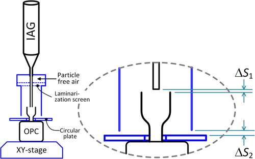
Figure 2. Inner dimensions of the isokinetic probe, which is an accessory of the DUT-OPC (Model ZN-PD50-S, OMRON).

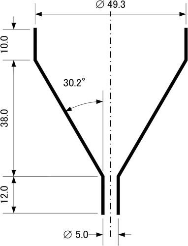
Table 1. Specifications of the OPC used in this study.

Manufacturer and model		Unit	OMRON, ZN-PD50-S
Sampling flowrate	Catalog	L/min	6
	Measured	L/min	6.03^a
Minimum detectable sizes		μm	5 and 10
Particle size channels	>5 μm	μm	5, 20, 50
	>10 μm	μm	10, 30, 50
Inner diameter of isokinetic probe		mm	49

^a Measured by using a large flow cell of a Gilibrator 2 (Gilian, USA). Measured flowrates are sensitive to the pressure drop across the attached flow measurement device.

The length from the bottom screen to the end of the chamber is 14.4 cm. This length is compared to the hydrodynamic entry length of a developing flow (White 1991), which is 240 cm. This indicates that the velocity profile in the tubular chamber is close to the plug flow. A circular plate is placed at the base of the isokinetic probe to create axi-symmetric velocity profile inside the chamber. The length of the gap between the end of the pipe and the plate, is set to 5 mm in this study to prevent the natural convection in the room air entering the chamber.

The inner diameter of the IAG exit tube used in this study is 4.6 mm, and the flowrate of the IAG, is set to 0.3 L/min. The length from the tip of the IAG exit tube to the inlet plane of the isokinetic probe, is set less than 2 mm. When the aerodynamic diameter of a particle is 15 μm the calculated stopping distance of the particle at the exit of the IAG tube is 0.024 mm, which ensures that inertial motion of the test particles has a negligible effect on particle trajectories; therefore, all test particles are entrained by the flow sampled into the isokinetic probe.

Simulating the sampling of uniformly mixed aerosol

Aerosol exits from the IAG through a tube, whose inner diameter is 4.6 mm, and the particles are most likely aligned near the centerline of the tube. If the centerline of the tube and the isokinetic probe are aligned, and if their positions remain fixed, then the particles will be concentrated at the centerline of the isokinetic probe. As is mentioned at the end of the Introduction section, such sampling setup is likely to cause the biases in the measured counting efficiencies unless aerosol flow mixes by turbulence after it is sampled into the probe. In this study, test particles are delivered to different positions over the inlet plane of the isokinetic probe to simulate the sampling of uniformly mixed aerosol in a real environment.

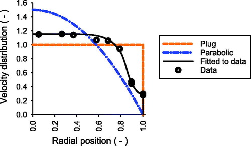
This study assumes that the distribution of particle flux (s⁻¹m⁻²) over the inlet plane is proportional to the flux of gas molecules (s⁻¹m⁻²). Assuming the specific volume of gas is constant over the inlet plane the gas flux is proportional to the velocity distribution of the air over the inlet. The average inlet velocity of the DUT-OPC of this study is about 0.05 m/s, and our hot-wire anemometer (Model 6034, Kanomax) cannot accurately measure such low value. Therefore, another OPC (RION KC-31 OPC) with average inlet velocity of 0.45 m/s is used instead.² Figure 3 shows an example of a measured velocity distribution over an isokinetic probe of the OPC. The graph also shows the velocity distribution of the plug and parabolic flows, where the plug and parabolic are theoretical distribution of inviscid flow and viscous flow, respectively. The measured distribution is in between plug and parabolic. The measurement is taken while the OPC is placed outside the laminar flow chamber. The measured distribution may be different if the measurements is taken while the OPC is placed inside the laminar flow chamber since the distribution is influenced by the flow inside the chamber. Nevertheless, this study assumes that the plug and parabolic flow bounds the true velocity distribution over an inlet plane of the isokinetic probe of a DUT-OPC. As it will be shown later in our uncertainty evaluation these two extreme flow profiles ensure that the uncertainty of is sufficiently large.

Figure 3. Measured velocity distribution over inlet plate of the isokinetic probe of an OPC (RION KC-31). The flowrate through the probe is 28.3 L/min. Plug flow and parabolic flow are the theoretical velocity distributions under inviscid and viscous flow, and they are assumed to be theoretical boundaries of the real velocity distribution.

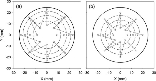
The IAG-generated particles are delivered to a set of points over the inlet plane to simulate the sampling of uniformly mixed aerosol in the chamber. Figure 4 illustrates two sets of points on the inlet plane of the isokinetic probe where test particles are delivered. Dashed lines are cross sections of streamlines in axi-symmetric coordinate system. Flow model is (a) plug flow and (b) parabolic flow, and the streamlines divide the total flowrate into four segments of equal flowrates. Test particles are delivered to radial positions which halves the flowrate in each equal-flow segment. Each equal-flow segment has eight injection points, and the same number of test particles are delivered at each point. In the delivery pattern under the parabolic flow assumption the streamlines are widely spaced near the wall since viscous effects at the wall reduce the velocity near the wall. Instead of moving the IAG, the OPC is placed on a metal plate which is attached to an XY-stage (Model OSMS26-100(XY), Sigma-Koki, Japan), and the plate is moved horizontally to deliver particles to a specific point. In this study, the speed of the XY-stage is set to 4 mm/s. The particle generation rate of the IAG is set to 30 s⁻¹, and 15 s is spent at each injection point. The total time is 9.0 min, and about 11% of the total time is spent for linear transportation of the stages. The particle generation process of the IAG is not paused during the linear transportation.

Figure 4. Injection points over the inlet plane of the isokinetic probe assuming the velocity distribution is (a) plug flow and (b) parabolic flow. Dashed lines are streamlines which divide the sampling flowrates into four equal segments. Open circles are points where test particles are delivered. Thin lines are routes taken to move through a set of delivery points.

Sizes of the IAG-generated particles

Sodium chloride (SC, Wako Pure Chemical, Japan) and lactose monohydrate (LM, Wako Pure Chemical) are the two particle materials used to evaluate the counting efficiencies in this study, and are 5.0 and 10 μm for both materials. SC is selected since its density value is expected to be accurate. LM is a common drug carrier in dry powder inhalers, and this study uses LM since IAG-generated particles of LM are relatively spherical as it will be shown later in our results.

The value of is calculated by (Iida et al. 2014; Minakami et al. 2017) (1a) (1b) where is the average mass of a particle (kg), and is the density of the particle material (kg/m³). The density values of SC and LM are assumed to be 2.170 and 1.547 g/cm³, respectively (CRC 2013). The particle mass is calculated from the mass fraction of the solute in the inkjet solution, , (kg-solute/kg-solution), and is the average mass of a droplet which is evaluated by measuring the mass of inkjet solution consumed from the reservoir bottle of the inkjet solution (Iida et al. 2014). The consumed mass divided by the number of droplets generated during the measurement gives the value of . The nozzle diameter of the inkjet head (Model MD-K-130, Microdrop Technologies GmbH, Germany) is 30 μm. The uncertainty of the is evaluated every time a new inkjet head is installed on the IAG. The sources of variation considered are the solute type and their mass fraction: two types of solutes (SC and LM), and two different values of . The values of are 0 and 13,000 mg/kg where latter concentration gives ≈ 9 μm and ≈ 10 μm when the particle materials are SC and LM, respectively. These solutions are different from those used during the evaluation of the . The symbol is the measured diameter of nonvolatile residue (m) when only the solvent (i.e. pure water) is used to generate droplets. A scanning electrical mobility spectrometer (Wang and Flagan 1990) was used to measure the size distributions of the nonvolatile residues.

An aerodynamic particle sizer spectrometer (APS, Model 3321, TSI, USA) was used to measure of the test particles.³ The value of of the test particles is determined as the diameter of PSL spheres whose light-scattering intensity would be the same as that of a given test particle, and is obtained from the relationship of the measured light-scattering intensity to the diameter for PSL spheres, which is determined separately in this study. Since the DUT-OPC in this study does not output the raw light-scattering signal, another OPC (RION KC-01D⁴) is used to obtain the value of of the test particles.⁵

Evaluation of the counting efficiencies

The counting efficiency of a DUT-OPC, , is defined as the ratio of the particle count rate of the OPC, , to the particle generation rate of the IAG, , which is set at 30 s⁻¹ in this study, that is, (2a) (2b) where is the particle counts reported by the OPC, , divided by the sampling time set to the OPC, . The value of is measured by the OPC.

The important difference from the parallel comparison method is that the values of evaluated by the IAG-based method are not expressed in terms of the particle number concentration. The counting efficiencies evaluated by the parallel comparison methods account for the error of sampled volume; this error occurs if there is a difference between the true flowrate and the flowrate that a DUT-OPC uses to calculate the sampled volume. If one needs to compare the values of evaluated by an IAG-based method to those evaluated by a parallel comparison method the true flowrate of the OPC needs to be measured independently by using a calibrated flowmeter. The counting efficiencies expressed in terms of concentration, , is given by (3) where is the true flowrate, and is the value that a DUT-OPC uses to calculate a sampled volume. This study only reports the counting efficiency in terms of particle count rate.

The measurement of is repeated six times for each particle delivery pattern shown in Figure 4. First, the average value is calculated for each delivery pattern ( and ). The final value of the counting efficiency, , is then calculated as the average of the two delivery patterns. (4a) (4b) (4c)

The value of is potentially different from the true value since the true value can be evaluated only if the true velocity distribution is known. The potential bias in is considered as a source of systematic error in our uncertainty analysis.

Uncertainty evaluation

In order to evaluate the uncertainty of the final value the error propagation is performed on the definition of the counting efficiency. (5)

The uncertainty factors of are the particle generation rate of the IAG and the average particle count rate, , where . The relative standard uncertainty (RSU) of the particle generation rate, , is about 0.26% (Iida et al. 2014; Minakami et al. 2017). The value of is assumed to have two uncertainty factors. The first factor is the repeatability of the particle count rate, . The second factor is the systematic effect in caused by the fact that the true velocity distribution over the inlet plane of the isokinetic probe is unknown, . (6)

The uncertainty from the measurement repeatability is evaluated by performing the analysis of variance (ANOVA). Input data to ANOVA consist of a set of in 6  2 matrix which consists of six repeated measurements of under two particle delivery patterns. The ANOVA is performed for every measurement condition: two particle sizes (= 5 or 10 μm), two particle types (SC or LM), and two minimum detectable sizes (= 5 or 10 μm).

One of the ANOVA outputs is the population variance due to repeatability, . The value of in Equation (6)(6) is estimated by (7) where is the total number of measurements which is 6  2 = 12 in this study.

The uncertainty due to the systematic error in the average particle count rate, , is estimated as follows. The probability density function of is uniformly distributed between the average count rates of the two particle-delivery patterns. (8a) (8b) where are the average values among six repeated measurements for the two particle-delivery patterns.

Results

Particle sizes

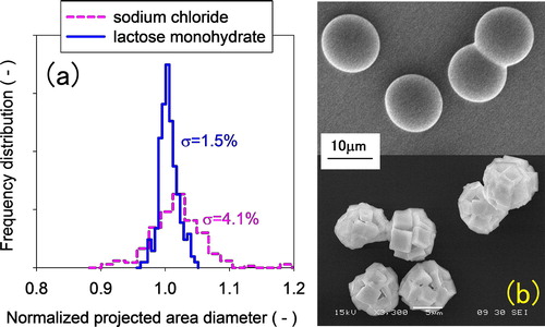
Figure 5a shows the size distribution of projected area diameter of SC and LM particles, and Figure 5b shows the images of LM and SC particles taken by using the scanning electron microscope (Minakami et al. 2017). LM particles are more spherical and monodisperse than SC particles are. The SC particles generated by the IAG are the agglomerates of smaller units of cubic crystals. The observed morphology of SC is expected when the diffusion of the solute in an evaporating droplet is significantly slower than the evaporation rate of the solvent (Baldelli et al. 2016).

Figure 5. (a) Particle size distributions of IAG-generated sodium chloride (SC) and LM particles. A scanning electron microscope (SEM) is used to measure their projected area diameters. The size axis is normalized by the average size. The average sizes of the distributions are 8.8 and 9.5 μm for SC and LM, respectively. (b) SEM images of LM (top) and SC (bottom) particles. Originally published in Earozoru Kenkyu (Minakami et al. 2017). Reproduced here with permission of the publisher.

The average droplet mass, , of the inkjet head in this study was 60.8 × 10⁻¹²kg, and its relative expanded uncertainty was 14% with the coverage factor (k) of 2. The diameter of the nonvolatile residue, , was 0.226 μm in mobility diameter, and its relative expanded uncertainty (k = 2) was 19%. These values are used to calculate in Equation (1)(1a) from a given value of . Table 2 summarizes the particle sizes of the IAG-generated particles in this study. For the same values of , LM and SC have similar ; however, of SC is significantly larger than of LM.

Table 2. Particle diameters of the IAG-generated particles.

, μm	Particle material	, mg/kg	, μm	, μm
5.0	Lactose monohydrate	1,655	6.0	4.7
	Sodium chloride	2,344	6.2	7.5
10	Lactose monohydrate	13,260	11.6	9.2
	Sodium chloride	18,480	12.2	14.4

Counting efficiencies

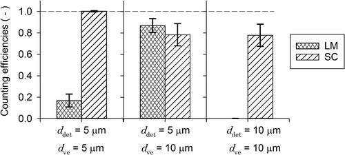
Figure 6 shows the value of which is the final value given by Equation (4c)(4c) . Minimum detectable size of the DUT-OPC, , is set to either 5 or 10 μm. When the values of and are equal, which are the left and right dataset of Figure 6, greater fractions of SC particles are detected. This trend is explained by the greater optical diameter of SC particles at 5 and 10 μm range as already shown in Table 2. At = 5 μm nearly 100% of SC particles are detected.

Figure 6. Counting efficiencies of the calibrated OPC (Model ZN-PD50-S, OMRON) for two different particle sizes and particle materials where LM and SC stand for lactose monohydrate and sodium chloride, respectively. The symbol is the minimum detectable size set to the OPC, and the symbol is the volume equivalent diameter of the IAG-generated particles. The error bars represent the expanded uncertainty (k = 2).

Figure 7 shows the values of and (Equations (4a)(4a) and (4b)(4b) ), which are the average counting efficiencies for two different particle delivery patterns. The figure also includes the average counting efficiencies when test particles are delivered along the z-axis of the isokinetic probe. Almost all SC particles with = 5 μm (or = 6.2 μm) are detected regardless of the delivery pattern. The results prove that the transport efficiencies through the isokinetic probe are nearly 100% when the aerodynamic diameters are less than 6.2 μm. decreases when is increased from 5 to 10 μm (middle dataset of Figure 6). The values of at = 10 μm are 78% and 87% for SC and LM, respectively, when the value of is set to 5 μm. A previous study evaluated of an OPC (Royco 220) over 2.5 to 15 μm particle diameter range (Liu, Berglund, and Agarwal 1974). The sampling flowrate of Royco 220 was at 2.83 L/min. of Royco 220 remains nearly constant for particles smaller than 6 μm while decreasing steadily with increasing particle diameter. Observed trends between these two studies are similar.

Figure 7. Counting efficiencies when the velocity distributions of the aerosol flow over the inlet plane of the isokinetic probe are assumed to be plug flow and parabolic flow. The figure also includes the value of when test particles are delivered along the center axis of the isokinetic probe. The error bars are two times the standard deviation of the mean value.

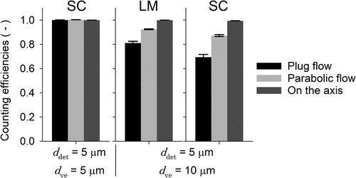
Our results indicate that the counting efficiencies depend on the delivery pattern. The radii of the delivery points are the largest among the three delivery patterns when the flow model is the plug flow. Counting efficiency is essentially 100% when all particles are delivered along the z-axis of the isokinetic probe. Similar results were obtained in our previous study, in which the IAG-generated particles are delivered along the center axis of the isokinetic probe of an OPC (RION KC-31) whose sampling flowrate is 28.3 L/min (Minakami et al. 2017). of 5 μm size channel range was 0.9998 on average, and its expanded uncertainty (k = 2) was 0.0052. The uncertainty is expected to increase if the sampling of uniformly mixed aerosol was simulated as it was done in this study.

Table 3 shows the summary of the uncertainty analysis of the reported counting efficiency, . At = 10 μm the largest source of the uncertainty is the systematic error, . That is, the delivery pattern affects the counting efficiency at = 10 μm. The table also gives the RSU of the Poisson sampling process, . The values are calculated by where is the average particle counts among twelve repeated measurements ( = 12). The underlined value shows that the uncertainty due to the repeatability, which occurs when the counting efficiency based on particle count rate is essentially 100%, is significantly smaller than those of the Poisson sampling process. As mentioned in the Introduction section, this is one important difference of the IAG-based method from the parallel comparison method. Sampling the entire population of the particles generated by the IAG is not a Poisson process; therefore, the uncertainty of the results does not have this particular random component.

Table 3. Summary of uncertainty analysis of the reported counting efficiency, .

Parameter	Symbol	Units	Values
Volume equivalent diameter		μm	5	5	10	10	10	10
Particle material	N/A		LM	SC	LM	SC	LM	SC
Minimum detectable size of the OPC		μm	5	5	5	5	10	10
Particle generation rate		s^−1	29.997	29.997	29.997	29.997	29.997	29.997
Sampling time		s	540	540	540	540	540	540
Total number of measurements		–	12	12	12	12	12	12
Average number of particle counts		–	2,740	16,229	14,073	12,688	25	12,607
Reported counting efficiency		–	0.169	1.002	0.869	0.783	0.0015	0.778
Uncertainty source	Symbol	Units	Values
Particle generation rate of the IAG		–	0.0026	0.0026	0.0026	0.0026	0.0026	0.0026
Repeatability of measurement		–	0.17	0.00029	0.0038	0.0074	0.087	0.0068
	[]		[0.0055]	[0.0023]	[0.0024]	[0.0026]	[0.058]	[0.0026]
Systematic effect on caused by the unknown velocity distribution of the aerosol		–	0.041	0.00082	0.037	0.066	0.16	0.066
Combined RSU of		–	0.18	0.0027	0.037	0.066	0.19	0.067

Discussion

The observed trend in implies that the inertial deposition of the particles is more significant when the particles are introduced at larger radius. Transport losses through the conical section of the isokinetic probe were estimated by using empirical equations which predict the inertial deposition in a flow constriction (Brockmann 2011). The Stokes number of the particles with = 15 μm was calculated from the average velocity at the inlet plane of the isokinetic probe and the diameter at the exit of the isokinetic probe. The value of Stokes number was 0.0071, and the calculated deposited fraction was 0.3%. The calculated result suggests that the inertial deposition on the conical wall of the isokinetic probe is negligibly small. On the other hand, the Stokes number at the exit of the isokinetic probe, which was calculated based on the average velocity and the inner diameter, was 0.68 which is large enough to induce significant inertial deposition when the streamline at a larger radial position makes a 30 degree turn at the end of the conical section of the probe (Figure 2). Lowering the angle from 30° to as low as 10° may reduce the transport losses (Liu, Berglund, and Agarwal 1974).

A paragraph is spent here to discuss whether it is possible to establish an equivalence between evaluated by the method given in ISO 21501-4 and the IAG-based method. The definition of particle size in ISO 21501-4 is the diameter of PSL spheres; therefore, the sizes of IAG-generated particles need to be expressed as to be consistent with ISO 21501-4. The value of can be adjusted to the size of PSL spheres by changing the of the inkjet solution; however, the of IAG-generated particles always has some error because the of IAG-generated particles are not as reproducible as the sizes of PSL spheres. In addition, the particle sizes based on other definitions (e.g. ) are also generally not equal between the PSL spheres and the IAG-generated particles. Regardless of these discrepancies in their particle sizes it is claimed that evaluated by the IAG-based method is reasonably equivalent to those obtained by using PSL spheres as long as values are evaluated over the same size range and the sizes of IAG-generated particles are expressed as . In the process of calculating the particle counts in difference-format may be summed across the size channels where the particle counts are expected to appear considering the value of and the size resolution of the OPC. Since is an adjustable parameter one good idea is to set the of IAG-generated particles at sufficiently larger sizes than the lower size-boundary of a given size channel considering the size resolution of the OPC and the size distribution of the IAG-generated particles.

The particle delivery process needs further improvement. The first development is to decouple the sampling time of the OPC and particle delivery process. The current process travels through a set of points, and the process is repeated until the iteration number reaches the desired number of measurements. In this process, the sampling time set to a DUT-OPC needs to be same as the time required to travel through a set of delivery points. There are various ways to synchronize the sampling setting of the OPC with the particle delivery process of the IAG; however, synchronizing these two devices requires some preparation prior to the evaluation of . The IAG-based method would be more practical if an arbitrary value could be set to the sampling time of a DUT-OPC while the particle delivery process is simulating the sampling of uniformly mixed aerosols. The second development is the particle delivery process to evaluate of light-scattering aerosol spectrometer (hereafter LSAS). The current particle delivery process cannot accurately evaluate of LSAS, whose ISO standard is ISO 21501-1 (ISO/TC24/SC4 2009). An example of aerosol spectrometers is WELAS (Palas GmbH). LSAS are designed to have high size resolution and are not designed to count all incoming particles. Their measuring volume is a small fraction of the sample flow. The delivery points shown in Figure 4 are too few to simulate the sampling of uniformly mixed aerosol through the measuring volume of LSAS. Further research and development are needed to evaluate of LASA by using the IAG.

Conclusion

It is challenging to aerosolize PSL spheres whose diameter is greater than 1 μm. Their particle number concentration tends to drift during nebulization of liquid suspension or fluctuate during the dry-dispersion. It is difficult to keep the amount of drift or fluctuation within a desirable range. A number of previous studies used particle material other than PSL to generate test particles whose diameter was greater than 1 μm. Regardless of the particle material the parallel comparison method has been used to evaluate the counting efficiencies of OPCs. This study uses the IAG as a method of evaluating the counting efficiencies. In this method, a DUT-OPC samples the entire population of the test particles generated by the IAG; therefore, the uncertainty of the particle counts does not have a random component caused by the Poisson sampling process. However, the IAG-generated particles tend to concentrate along the centerline of a tube when the particles exit the IAG housing; therefore, the particles are not well-mixed in the sampled aerosol. This study introduces a method to deliver test particles to different points over the inlet plane of the isokinetic probe to simulate the sampling of uniformly mixed aerosol from a real environment.

This study demonstrates the IAG-based method and evaluates the values of at = 5 and 10 μm. The test particles are composed of LM or SC. When the values of and are equal the counting efficiency depends on the particle material, and the greater fraction SC particles are detected since their value of is greater than LM particles. The counting efficiencies at 10 μm depend on the flow model used to simulate the distribution of particle flux into the isokinetic probe. The results indicate that the counting efficiency at this size is potentially different from the true value since the true value can be evaluated only if the true velocity distribution is known. The potential bias in the counting efficiency is considered as a source of systematic error in our uncertainty analysis.

Acknowledgments

Figure 5 was derived from figures originally published in Earozoru Kenkyu, the official journal of the Japan Association of Aerosol Science and Technology (Minakami et al. 2017). The authors would like to thank the journal for permission to reproduce these figures.

Disclosure statement

No potential conflict of interest was reported by the authors.

Notes

1 The acronym DUT is added to indicate that the OPC is the device under test.

2 The sampling flowrate of RION KC-31 is 28.3 L/min, and the inner diameter of its isokinetic probe is 36.5 mm. The inlet plane of the isokinetic probe is hypothetically divided into two hemispheres. Velocity is measured at different points along the straight segment of the hemisphere.

3 PSL spheres are used to calibrate the aerodynamic size channels of the APS. The d_ae in this study is defined at where the number-based cumulative frequency distribution is at 50%.

4 The wavelength of the incident light is 780 nm. The detector angle is 70° from the forward direction.

5 Representative light-scattering intensity is defined at where the frequency distribution of the measured light scattering intensity is at 50%.

References

- Auderset, K., G. Baur, M. Ess, A. Kimàk, F. Lüönd, and K. Vasilatou. 2012. Calibration of optical particle counters. 2017. Accessed December 23, 2017. https://www.metas.ch/metas/en/home/fabe/partikel-und-aerosole.html
- Baldelli, A., R. M. Power, R. E. H. Miles, J. P. Reid, and R. Vehring. 2016. Effect of crystallization kinetics on the properties of spray dried microparticles. Aerosol Sci. Technol. 50 (7):693–704. doi:10.1080/02786826.2016.1177163.
- Bemer, D., J. F. Fabries, and A. Renoux. 1990. Calculation of the theoretical response of an optical particle counter and its practical usefulness. J. Aerosol Sci. 21 (5):689–700. doi:10.1016/0021-8502(90)90123-F.
- Berglund, R. N., and B. Y. H. Liu. 1973. Generation of monodisperse aerosol standards. Environmental Sci. Technol. 7 (2):147–53. doi:10.1021/es60074a001.
- Binnig, J., J. Meyer, and G. Kasper. 2007. Calibration of an optical particle counter to provide PM2.5 mass for well-defined particle materials. J. Aerosol Sci. 38 (3):325–32. doi:10.1016/j.jaerosci.2006.12.001.
- Bottiger, J. R., P. J. Deluca, E. W. Stuebing, and D. R. Vanreenen. 1998. An ink jet aerosol generator. J. Aerosol Sci. 29:S965–S6.
- Brockmann, J. E. 2011. Aerosol transport in sampling lines and inlets, In Aerosol measurement: Principles, techniques, and applications, ed. P. Kulkani, P. Baron, and K. Willeke, 69–105. Hoboken, NJ: John Wiley & Sons.
- Chen, B. T., Y. S. Cheng, and H. C. Yeh. 1984. Experimental responses of two optical particle counters. J. Aerosol Sci. 15 (4):457–64. doi:10.1016/0021-8502(84)90041-7.
- Cobo, F., G. N. Stacey, J. L. Cortés, and Á. Concha. 2006. Environmental monitoring in stem cell banks. Appl. Microbiol. Biotechnol. 70 (6):651. doi:10.1007/s00253-006-0326-5.
- CRC. 2013. Section 3: Physical constants of organic compounds. In CRC handbook of chemistry and physics (dvd version 2013), ed. W. Haynes. 93rd edn. Boca Raton, FL: CRC Press/Taylor and Francis.
- Duan, H., F. J. Romay, C. Li, A. Naqwi, W. Deng, and B. Y. H. Liu. 2016. Generation of monodisperse aerosols by combining aerodynamic flow-focusing and mechanical perturbation. Aerosol Sci. Technol. 50 (1):17–25. doi:10.1080/02786826.2015.1123213.
- Heim, M., B. J. Mullins, H. Umhauer, and G. Kasper. 2008. Performance evaluation of three optical particle counters with an efficient “multimodal” calibration method. J. Aerosol Sci. 39 (12):1019–31. doi:10.1016/j.jaerosci.2008.07.006.
- Iida, K., H. Sakurai, K. Saito, and K. Ehara. 2014. Inkjet aerosol generator as monodisperse particle number standard. Aerosol Sci. Technol. 48 (8):789–802. doi:10.1080/02786826.2014.930948.
- ISO/TC24/SC4. 2007. ISO 21501-4: Determination of particle size distribution – Single particle light interaction methods – Part 4: Light scattering airborne particle counter for clean spaces.
- ISO/TC24/SC4. 2009. ISO 21501-1: Determination of particle size distribution – Single particle light interaction methods – Part 1: Light scattering aerosol spectrometer. Geneva, Switzerland: International Organization for Standardization.
- Kesavan, J. S., J. R. Bottiger, D. R. Schepers, and A. R. McFarland. 2014. Comparison of particle number counts measured with an ink jet aerosol generator and an aerodynamic particle sizer. Aerosol Sci. Technol. 48 (2):219–27. doi:10.1080/02786826.2013.868594.
- Liu, B. Y. H., R. N. Berglund, and J. K. Agarwal. 1974. Experimental studies of optical particle counters. Atmos. Environ. (1967) 8 (7):717–32.
- Mäkynen, J., T. Hakulinen, M. Kivistö, and M. Lehtimäki. 1982. Optical particle counters: Response, resolution and counting efficiency. J. Aerosol Sci. 13 (6):529–35. doi:10.1016/0021-8502(82)90018-0.
- Minakami, T., T. Hosokawa, K. Kondo, K. Iida, K. Ehara, and H. Sakurai. 2017. Evaluation of counting efficiencies for optical particle counters by using inkjet aerosol generator. Earozoru Kenkyu 32 (1):29–36. doi:10.11203/jar.32.29.
- Mirhoseini, S. H., M. Nikaeen, H. Khanahmd, M. Hatamzadeh, and A. Hassanzadeh. 2015. Monitoring of airborne bacteria and aerosols in different wards of hospitals – Particle counting usefulness in investigation of airborne bacteria. Ann. Agric. Environ. Med. 22 (4):670–3. doi:10.5604/12321966.1185772.
- Raval, J. S., E. Koch, and A. D. Donnenberg. 2012. Real-time monitoring of non-viable airborne particles correlates with airborne colonies and represents an acceptable surrogate for daily assessment of cell-processing cleanroom performance. Cytotherapy 14 (9):1144–50. doi:10.3109/14653249.2012.698728.
- Shin, W. J., Y.-S. Jeong, K. Choi, and W. G. Shin. 2015. The effect of inkjet operating parameters on the size control of aerosol particles. Aerosol Sci. Technol. 49 (12):1256–62. doi:10.1080/02786826.2015.1115465.
- Stolzenburg, M., N. Kreisberg, and S. Hering. 1998. Atmospheric size distributions measured by differential mobility optical particle size spectrometry. Aerosol Sci. Technol. 29 (5):402–18. doi:10.1080/02786829808965579.
- Wang, S. C., and R. C. Flagan. 1990. Scanning electrical mobility spectrometer. Aerosol Sci. Technol. 13 (2):230–40. doi:10.1080/02786829008959441.
- Wen, H. Y., and G. Kasper. 1986. Counting efficiencies of six commercial particle counters. J. Aerosol Sci. 17 (6):947–61. doi:10.1016/0021-8502(86)90021-2.
- White, F. M. 1991. Viscous fluid flow. New York: McGraw-Hill.