Scanning DMA data analysis II. Integrated DMA-CPC instrument response and data inversion

Abstract

Analysis of scanning electrical mobility spectrometer (SEMS) or SMPS data requires coupling the scanning differential mobility analyzer (DMA) transfer function with the response functions for the instrument plumbing and the detector. In the limit of plug flow (uniform velocity) within the DMA, the scanning DMA transfer function has the same form as that for constant voltage. Most SEMS/SMPS data analysis uses this model, though previous studies have shown that boundary layers distort the transfer function during scanning DMA measurements. Part I determined the instantaneous transfer function during scanning of the TSI Model 3081 A long column DMA by modeling the flows, fields, and particle trajectories within the actual DMA geometry. This study (Part II) combines that transfer function with empirical data on the efficiencies and delay time distributions of the plumbing and detector of the SEMS/SMPS to determine the instantaneous rate at which particles are counted, and integrates the count rate over the finite counting time interval to obtain the integrated SEMS/SMPS response function. Simulations using this geometrical model are compared with those obtained using traditional, idealized DMA models for scan rates ranging from slow (240 s) to very fast (10 s), and with measurements of monodisperse calibration aerosols. Data inversion studies show that both increasing and decreasing voltage scans can be used to determine the particle size distribution, even with fast scans.

Copyright © 2018 American Association for Aerosol Research

EDITOR:

• Jingkun Jiang

1. Introduction

Measurement of particle size distributions using the differential mobility analyzer (DMA) requires knowledge of the particle behavior within the charge conditioner, DMA, particle detector, and all plumbing in between. When measurements are made in a series of constant voltage steps, as in the differential mobility particle sizer (DMPS), these components can be treated separately because the measurement is made with each component operating at steady-state. The acquired data in this stepwise operation are particle counts, , measured in a finite counting time, , at each of the voltage settings, V_i. For an incoming aerosol sample flow rate, , and a steady particle size distribution, , the counts acquired using a condensation particle counter (CPC) detector are (1) where the so called transfer function of the DMA, , is the probability that a particle of diameter, D_p, that carries elementary charges, and, hence, has mobility , will be transmitted through the classification region of the DMA operated at voltage V_i. If the incoming aerosol sample flow, , and outgoing classified sample flow, , are balanced, i.e., , the peak in the transmission efficiency occurs at the mobility of a particle that is transmitted from the centroid of the incoming aerosol flow, to the centroid of the classified aerosol outlet flow. Knutson and Whitby (1975) showed this centroid mobility for nondiffusive particles to be ; and denote the sheath and exhaust flow rates through the DMA, respectively, and L is the length of the classification region. The transfer function also depends on the flow rate ratios, , and . Stolzenburg (1988) derived an elegant expression for the transfer function that includes the effects of Brownian diffusion on the steady-state transmission efficiency through the classification region of the constant-voltage DMA. This transfer function forms the basis for DMPS data inversion to find from the set of measured counts, .

The counts recorded also depend on the efficiency of particle transmission through the entrance and exit regions of the DMA, and , respectively, that of the flow passages upstream and downstream of the DMA (including the charge conditioner), , the counting efficiency of the CPC, , and the probability that a particle will acquire elementary charges, . The transmission efficiencies may depend on charge state because the aerosol must pass through a transition between the high voltage used in the classification and ground somewhere in the system; for the most common DMAs, that transition occurs within the exit flow passages of the DMA, though some DMAs have that transition at the entrance. Charge may also affect the detection efficiency of the CPC due to its influence on particle activation.

A key challenge in measuring particle size distributions by stepping the voltage is the substantial time that one must wait after stepping the voltage to allow steady-state to be achieved, thereby slowing the acquisition of the particle size distribution. Scanning the DMA voltage eliminates those delays, enabling rapid particle size distribution measurements (Wang and Flagan 1990). In the limit of plug flow (uniform velocity) between the classification electrodes, this scanning electrical mobility spectrometer (SEMS; also known as the scanning mobility particle sizer, SMPS) yields the same nondiffusive transfer function as the DMPS. However, the transfer function must be evaluated at the mean field strength (voltage) experienced by a particle during its transit through the classification region of the DMA. The authors have encountered situations in which the transfer function was evaluated at the voltage corresponding to the time at which a particle exits the DMA rather than at the mean voltage. Because this closely parallels the DMPS analysis, we label this erroneous estimation the static transfer function; results for this evaluation will be shown to illustrate the substantial bias that it introduces. We also note that, due to laminar flow in the DMA, the plug-flow limit can be approximated only at very high Reynolds numbers.

In the first field deployment of the SEMS, Russell, Flagan, and Seinfeld (1995) observed an asymmetric response between scans in which the voltage was increased in an exponential ramp (up-scan) and those in which the voltage was exponentially decreased (down-scan); this distortion was attributed to the relatively slow response of the CPC that was used to detect the transmitted particles. Mixing within the CPC itself leads to a distribution of residence times that cause particle counts to be spread over many later time bins than that in which they would have been detected with an ideal, fast-response detector. Previous studies used a continuously stirred-tank-reactor (CSTR) plus plug flow reactor (PFR) model to describe the distribution of delay times within the CPC (Russell, Flagan, and Seinfeld 1995; Collins, Flagan, and Seinfeld 2002). This model predicts that the residence time distribution function that describes the probability that a particle that enters the CSTR at time t = 0 will remain within the CSTR at time t is (2) where and are the mean delay time in the CSTR and PFR, respectively. Thus, a step change in concentration from N₀ to N₁ after an initial plumbing delay of time leads to a linear decay of with time, t, The slope of the decay is .

The mathematical model of the SEMS system response developed in that study was quite complex; Collins, Flagan, and Seinfeld (2002) later developed a simpler deconvolution algorithm to attribute the particle counts to the proper counting-time bins. Treatment of the effects of slow detector response on the size distributions inferred from SEMS data improved the ability of the instrument to make quantitative measurements.

Most SEMS/SMPS data analysis follows the original Wang and Flagan (1990) approach, though some researchers do account for the CPC time response using the method of Collins, Flagan, and Seinfeld (2002). As will be shown below, the use of the transfer function for constant voltage classification in combination with the correction for the finite time response of the CPC is reasonable for sufficiently slow scans in which the voltage remains essentially constant during a particle’s transit through the DMA. Unfortunately, correction for the slow detector response fails to capture all of the differences between the SEMS or SMPS and the DMPS. Using Brownian dynamics simulations, Collins et al. (2004) demonstrated that the presence of boundary layers within the classification region alters the trajectories and time required for a particle to traverse the length of the classifier. An analytical solution for the nondiffusive transfer function has been derived to describe scanning of a cylindrical DMA(Dubey and Dhaniyala 2008; Mamakos, Ntziachristos, and Samaras 2008) in the limit of the idealized, laminar, parallel-flow cylindrical DMA (PFDMA-L); the influence of particle diffusion in this model was later simulated using Brownian dynamics (Dubey and Dhaniyala 2011).

In Part I of this two-part series of papers, Mai and Flagan (in press) use finite element simulations to capture the details of the flows and electric field within an actual, cylindrical DMA (the TSI Model 3081 long column DMA). These fields were combined with Brownian dynamics simulations of diffusive particle transport through the scanning DMA. They found it necessary to extend the classification region model to include portions of the inlet and exit regions of the DMA in the numerical evaluation of the transfer function, because laminar flow within the narrow aerosol inlet annulus of the TSI DMA alters the velocity distribution at the entrance to the classification region, and, thereby, some particle trajectories. The flow fields within the DMA are sufficiently complex that particles of a given mobility that enter the classification region at different times can exit a voltage-scanning DMA at the same time. In addition, the exit region introduces a range of delays between the time that a particle exits the space between the electrodes and their exit from the DMA itself. Hence, the transfer function for the SEMS can no longer be considered to be the probability of transmission; indeed, under some circumstances, the instantaneous transfer function of a DMA that is operated in scanning mode can exceed unity.

The scanning DMA transfer function is the starting point for describing the SEMS, or for the analyzing data produced by these instruments. Here, we develop the integrated system response function and the corresponding data inversion methodology for scanning DMA measurements in the context of measurements made using the TSI Model 3081 A long-column DMA with a TSI Model 3010 CPC used as the detector. The specific operating parameters considered are those employed in measurement of secondary organic aerosol yields in chamber studies at Caltech, which, because aerosol yield is a measure of mass conversion, focuses on large particles. An observed tail of the up-scan (increasing voltage) transfer function toward large particles introduces uncertainities in yield estimates that have prompted our reanalysis of the instrument response function. Nonetheless, the methodology described below is applicable to other mobility classifiers and detectors, and to measurements in other size ranges, but consideration of all possible operating parameters is beyond the scope of this study. To determine the response function of the integrated measurement system, the instantaneous DMA transfer function must be known; in Part I, Mai and Flagan (in press) have determined it for the particular operating conditions that we examine here. Upstream plumbing and components such as the charge conditioner also affect the ultimate detection efficiency due to losses and the charge distribution attained. All of these factors need to be integrated into the instrument response kernel to enable data inversion for particle size distribution determination.

2. Methods

2.1. Instantaneous and integrated SEMS/SMPS transfer functions

A particle’s size and charge determine its electrical mobility, , and Brownian diffusivity, , where k, T, and e are the Boltzmann constant, temperature, and elementary unit of charge, respectively. Thus, the mobility and charge provide the information required to describe its behavior in the DMA. Assuming that the particle size distribution is steady, the instantaneous transfer function of the scanning DMA can be defined as (3) where , and denotes the time-in-scan, i.e., the difference between the time at which the particle exits the DMA and the time at which the measurement cycle started, t₀. Because the voltage changes continuously with time, is related to the mobility of the particles that are optimally transmitted through the voltage program V(t). Particle losses, as well as any delays in the transit of particles from the entrance to the exit of the classifier, have also been incorporated into the instantaneous SEMS/SMPS transfer function because they are affected by the voltage scan. These intra-DMA delays, which add to the signal smearing due to the CPC and other downstream components, have not been considered in previous studies.

Mai and Flagan (in press) in Part I used Brownian dynamics simulations to find the instantaneous transfer functions for two DMA models: (i) the idealized laminar PFDMA in which the flow is described by the analytical solution for fully developed laminar flow between coaxial cylinders, leading to transfer function, ; and (ii) real flow fields derived from finite element simulations of the actual geometry of the specific DMA being studied (G-DMA), the TSI Model 3081 long-column DMA, . Losses and time delays in the entrance and exit regions of the DMA are incorporated into , as are losses to the walls of the classification region. To fully capture the effects of the real geometry, the classification region was extended beyond the space between the electrodes to include portions of the entrance and exit regions of the DMA that influence classification.

The introduction of the SEMS (Wang and Flagan 1990) considered an even simpler idealized, parallel-flow model, i.e., one with uniform velocity (plug flow) for which the nondiffusive transfer function for plug-flow within the SEMS, reduces to that derived by Knutson and Whitby (1975) for the DMPS; particle diffusion can be included by replacing the nondiffusive transfer function with the diffusive one (Stolzenburg 1988), provided it is applied at the mean voltage that a particle experiences during its transit through the classification region; thus, Brownian dynamics simulations are unnecessary for plug flow (Mai and Flagan in press). Rather than evaluate the mean voltage, it may tempting to simplify this model by relating the mobility to the voltage at the instant of time when a particle is detected, but this introduces an additional large bias as will be shown below.

2.2. Integrated system transfer function for the SEMS

Combining the instantaneous transfer function for the scanning DMA with the response functions for the downstream components provides the information needed to describe the integrated system. In the SEMS/SMPS, counts are acquired in successive time bins of duration , but without the intervening delay between counting intervals that is required to attain steady-state in DMPS measurements. To understand the integrated system performance, the voltage program that comprises a scan must first be defined.

The time bins are defined from the start of the voltage measurement cycle, which begins at global time for the scan. The time-in-scan, t, is defined such that . Initially, the voltage is held constant at the minimum voltage of the measurement cycle, (which may be either positive or negative, depending on the polarity of the particles being classified), for time to ensure that no particles from the previous scan remain in the classification region to be included in the counts for scan ν. The voltage is then ramped exponentially to the maximum (positive or negative) voltage, , in time , held constant at to ensure that all particles that entered the classification region during the up-ramp are counted, and then ramped exponentially back to in time .

The applied voltage cycle is, thus, (4)

The exponential ramp time constant, , is given by . The total measurement cycle time, or scan time, is (5) and . Owing to the asymmetry in the signals measured in the down-scan as compared to the up-scan, many users do not use results obtained from the down-scan and, therefore, make as short as possible. For convenience in data acquisition and control, the different process times, , etc., are usually specified as integer multiples of the detector counting time, .

The rate at which particles of log-mobility u are counted into a SEMS time bin results from a convolution of the rate at which particles that exit the classifier at all earlier times with the downstream delay time distribution function, assuming a quasi-steady-state size distribution, (6) where denotes the convolution operator which is defined (Bracewell 1986) such that (7) with the lower bound on the integral through all past time. In practice, the integral has finite values only after some early time that we may define as t = 0. The period during which the voltage is held constant at a low (high) voltage before the start of a voltage ramp is selected such that the start of the holding period can be taken as t = 0 for an up-scan (down-scan). This convolution forms the instantaneous transfer function for the SEMS, i.e., (8)

The total number of particles recorded in time bin i, i.e., in the time interval , is obtained by integrating the particles transmitted at any instant of time over the counting-time interval, , i.e., (9)

For a steady size distribution, only the instantaneous system transfer function depends upon time. Hence, a cumulative, integrated system transfer function can be defined as (10)

If is sufficiently long for all particles that entered the DMA during previous scans to be cleared from the measurement system before the start of the voltage up-ramp, the lower bound on the integral can be taken to be t = 0. Substituting Equation (9)(9) into Equation (10)(10) yields (11)

Note that, because of the varying delays that different particles may experience, the counting bins are not synchronized with particular voltages in the measurement cycle, i.e., the voltage at the instant at which a particle is counted is not simply related to its size.

Grouping all factors other than the size distribution into the kernel function, i.e., (12) the particle count becomes (13)

We seek to determine the particle size distribution, from the counts recorded in the various time bins throughout the voltage scan, i.e., from the signals . To do this, we need to discretize the particle size distribution, , where N denotes the total number concentration of particles of all sizes. Numerous representations of the particle size distribution have been employed in previous studies, including: (i) modal models in which is described by a collection of log-normal modes, (ii) so-called nodal representations in which the size distribution is approximated by delta-functions at a set of J discrete sizes, (iii) sectional models (histograms), in which the size distribution is assumed to be constant within each size interval between discretization points, and (iv) linear-splines. As noted by Wolfenbarger and Seinfeld (1990), other basis functions such as cubic splines might be more realistic, but would introduce the need for nonlinear constraints to ensure non-negative size distributions, whereas linear splines require only linear constraints to obtain realistic results. For the nodal and sectional models, the size distribution can be taken outside the integral. On the other hand, modal, linear spline, or higher order models require integration over the functional form of the discretized size distribution. Hence, aerosol measurements are generally inverted using nodal or sectional representations of the size distributions.

As the linear spline model allows good fidelity with the actual size distribution without imposing an arbitrary shape to the particle size distribution, we employ the linear-spline representation on discretization points . The particle size distribution thus becomes (14)

To improve accuracy, we discretize the integral in Equation (13)(13) over a finer grid than that used for the size distribution. The increment in particle size may be abbreviated as . Using the linear-spline representation of the size distribution, and carrying out the integration over u using the trapezoidal rule over the integration diameter space, Equation (13)(13) thus becomes (15) where (16) is the weighting factor arising from the trapezoidal integral. The instrument response as a function of size distribution thus becomes (See Supplementary Information for derivation) (17)

To determine the values of the size distribution at the discretization points, , we must solve the system of equations (18) where the kernel function is defined as (19)

Thus, we seek to solve for the values of the size distribution parameters ; is the array of the count data, . We employ a non-negative least squares algorithm (Merritt and Zhang 2005), and compare results obtained using the DMA transfer functions obtained with three DMA models: (i) the geometric model (G-DMA) that is based upon the actual instrument design (TSI Model 3081 A long-column DMA, with instantaneous transfer function ), (ii) the laminar, parallel-flow DMA model (transfer function: ), and (iii) the uniform velocity (plug flow) model using the Stolzenburg (1988) transfer function evaluated at the mean voltage experienced by a particle during its passage through the classification region (transfer function: ). One additional model is presented since a natural misinterpretation of SEMS/SMPS performance is to consider the classification voltage to be that at the instant when the particle leaves the classifier; we have labeled this model the static-DMA transfer function, and evaluated it by applying the diffusional transfer function (Stolzenburg 1988). Plumbing delays downstream of the DMA could further aggravate the biases associated with this misinterpretation of the scanning DMA method.

2.3. Experimental validation of integral instrument response function

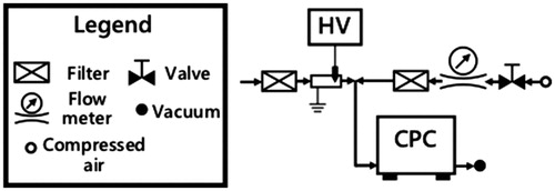
The time response of a component in the SEMS measurement system can be directly measured by subjecting it to a transient source, either a step change in concentration produced by switching the flow between a particle-free one and one containing particles (Quant 1992; Hering et al. 2005), or by producing a pulse of particles by, for example, generating a weak spark that will ablate some electrode material and nucleate fine particles in the flow (Wang et al. 2002). The latter approach minimizes perturbations to the flow, so we have employed it to measure the time response of the components downstream of the DMA outlet in our SEMS instrument, including the plumbing that connects the DMA outlet to the inlet of a TSI 3010 CPC. A computer-triggered spark-source was installed at the entrance of that plumbing (see Figure 1). The detector was operated at the same flow rate, and saturator and condenser temperatures used in SEMS measurements of particle size distributions. LabView software was used to control the spark and record particle counts into 0.1 s time bins. The size-dependent detection efficiency of this system was calibrated against a recently calibrated TSI 3010 CPC.

Figure 1. Experimental setup schematic to measure the CPC residence time distribution.

Figure 2 illustrates the experimental system that was used to validate the integral instrument response function. Polystyrene latex (PSL) calibration particles were nebulized, neutralized using a TSI 3077 Kr-85 charge conditioner, and then classified using a TSI 3081 A DMA (DMA₁) that was operated at constant voltage to produce a monodisperse calibration aerosol. The particle number concentration downstream of DMA₁ was monitored with a TSI 3760 CPC (CPC₁), operated at a sample flow rate of 1.51 LPM (liters per minute). DMA₁ was operated with equal aerosol and classified sample flow rates (i.e., balanced flows) of 1 LPM, and sheath and exhaust flow rates of 5 LPM. The voltage of DMA₁ was set to maximize the particle concentration. The classified PSL particles were subjected to bipolar diffusion charging using a home-made soft-X-ray charge conditioner, and then analyzed using a SEMS/SMPS system consisting of a TSI 3081 A DMA (DMA₂) with a TSI 3010 CPC detector (CPC₂; sample flow rate 0.975 LPM); the operating parameters for these measurements are summarized in Table 1. The counting time for CPC₂ was = 0.5 s, while the reference CPC (CPC₁) recorded the particle concentration at 1 s intervals. Prior to these measurements, the counting efficiencies of the two CPCs were compared and tuned to ensure consistent concentration measurements.

Figure 2. Experimental setup schematic to measure the DMA-CPC composite instrument response.

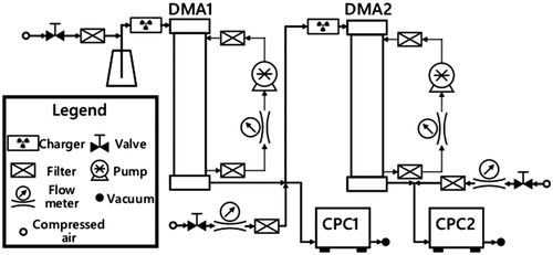
Table 1. Operating parameters for the scanning DMA.

Parameter	Notation	Value
Length	L	44.38
Inner radius (CM)	R1	0.937
Outer radius (CM)	R2	1.961
Polydisperse flow rate (LPM)	Qa	0.515
Monodisperse flow rate (LPM)	Qc	0.515
Sheath flow rate (LPM)	Qsh	2.510
Excess flow rate (LPM)	Qex	2.510
Low electrode voltage (V)	Vlow	15
High electrode voltage (V)	Vhigh	9,850
Up scan time (s)	tramp,u	10, 20, 45, 90
Down scan time (s)	tramp,d	10, 20, 45, 90
Holding time at Vlow	tlow	20
Holding time at Vhigh	thigh	20

3. Results

3.1. CPC response time distribution

Figure 3 shows the measured response time distributions from 600 spark-pulse events, with cumulative counts exceeding 10⁵. The CPC sample flow was 0.975 LPM, leading to an estimated mean residence time of particles in the downstream plumbing and CPC of 2.36 s. The time-response data were fitted to two different models that are described below. In each case, the fits were weighted according to Poisson statistics based on the counts recorded in each time bin, i, such that the variance in the counts, , where c_i is the number of counts in time bin i. Following Russell, Flagan, and Seinfeld (1995), the first model treats the CPC response as a PFR in series with a continuous stirred-tank reactor (CSTR), leading to the residence time distribution given by Equation (2)(2) . Global optimization of the weighted least-squares fit between experimental data and yielded s, and s as shown by the dashed line in Figure 3, however, the PFR + CSTR model fails to capture the tail at long times.

Figure 3. Residence time distribution of TSI 3010 CPC, with sampling flow rate of 0.975 LPM.

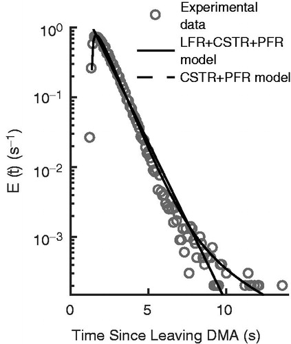
The plumbing connections between the DMA and CPC, and parts of the flow within the CPC employed in this study, can be described using a laminar-flow (LF) model, which has a residence time distribution of

Passages within the CPC may add additional LF-like delay distributions. Adding a LF in series with the CSTR and PFR allows the model to capture the long-time tail of the response; the combined delay time distribution then becomes , or (20)

where is the exponential integral. The time scales obtained by weighted fitting to the experimental data are s, s and s. This three-parameter delay time distribution captures the long-time tail in up-scan measurements, making it possible to properly attribute contributions of the tail of the response distribution to appropriate mobilities (or sizes) and, thereby, correct a potential overestimation of the aerosol mass that is very important to chamber measurements of aerosol yield.

3.2. Integrated SEMS response function

Substituting the CPC time response function, numerical results from direct measurement or empirical fit to Equation (20)(20) , into Equation (8)(8) yield the integrated SEMS system response function, . To examine how well the idealized laminar and plug-flow models, and the one based on the geometry of a real DMA, G-DMA, describe measurements, we seek to compare predicted particle counts for measurements of monodisperse PSL particles to experimental observations, using Equation (11)(11) . The transmission efficiency of the flow system, , remains unknown, however. The losses for which accounts are not directly associated with the scan, so they should not depend upon the scan rate. To enable comparison between models, we estimate this parameter by using it as the single parameter in fitting the time variation of ratio of the particle number concentration predicted for the G-DMA model to the particle number concentration that enters the DMA during a counting-time interval, i.e., we find the value of for which , where is the number concentration of the monodisperse particles upstream of the SEMS system. The G-DMA model was selected for this fitting because, as will be shown below, it most closely approximates the observed time variation while other models exhibit notable time shifts. The resulting concentration ratios are shown for both up-scans and down-scans and for a range of scan rates as discussed below.

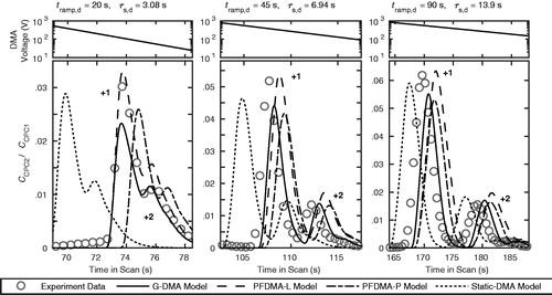
Figure 4 compares measured and observed ratios for 147 nm PSL particles of duration . These correspond to exponential scan time constants ranging from 1.54 s to 13.9 s. The concentrations display two major peaks due to the presence of multiply-charged particles in the aerosol processed through the charge conditioner. The larger peak is associated with singly-charged particles; the lower peak precedes it due to the higher mobility of the doubly charged () particles. As the scan rate increases, peaks associated with particles of charge states merge because resolution decreases due to the distribution of delays within components of the measurement system, particularly the CPC. The peak particle concentration ratio also decreases in the fast scan because the transmitted particles are redistributed among an increasing number of time bins. For example, the maximum concentration ratio for singly-charged, 147 nm particles is 0.06 for = 90 s, but decreases to 0.03 for = 10 s. In short, fast scans come at a cost of reduced resolution and particle concentration ratio.

Figure 4. Up-scan experimental and modeling results for SEMS instrument response to monodisperse 147 nm particles with ramp duration = 10, 20, 45, and 90 s (corresponding to scan time = 1.54, 3.08, 6.94, and 13.9 s).

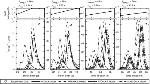
Using the charge distribution reported by Leppä et al. (2017) for , each of the models predicts multiple peaks as observed experimentally, though the times at which they appear differ. For the slowest scan (90 s) the G-DMA model closely approximates the appearance time and magnitude of the experimentally observed count ratio for the singly charged peak; the peak value is overestimated, suggesting that the charge distribution produced by the new soft x-ray charger used in these experiments may differ from that which we have assumed. The predictions of the G-DMA model capture the variation in the recorded signals for scans as short as 10 s, though the peaks are poorly resolved for such fast scans.

The values of the particle-concentration ratios are low (< 0.1) due, in large part, to the charging probability that results from bipolar diffusion charging, though particle losses also contribute. The fitted values of , summarized in Table 2, include losses both in the plumbing upstream of the DMA classification region, and in the new charge conditioner. The values obtained were about 0.7 for each particle size examined (147 nm, 296 nm, and 498 nm). Any deviations from the assumed size-dependent charging probability will also be included in the values of determined during the data fitting. The peak ratios predicted for singly-charged particles using the parallel-flow models are slightly higher than observed due to losses in the extended entrance region of the G-DMA model used in the fitting of that do not occur in the PFDMA models. In addition, the predicted widths of the parallel-flow model peaks are narrower than for the G-DMA model, further enhancing the peak height. The apparent dependence of on scan time likely results from decreased resolution during fast scans; hence, values obtained in the slowest scans ( = 90 s) are most reliable, particularly since these losses occur upstream of the classification and, therefore, are not affected by the scanning operation. The fitted flow-system penetration efficiency does not show a significant dependence on particle size, which is not surprising since the PSL particle sizes are sufficiently large that diffusion does not significantly affect their transmission. The relatively low penetration efficiency is likely due to the prototype soft X-ray charge conditioner used in these tests.

Table 2. Penetration efficiencies through the flow system for the geometric model (G-DMA) for various particle sizes.

Dp (nm)	Up-scan ηF	Down-scan ηF
147	0.706 0.008	0.647 0.016
296	0.7220.005	0.694 0.012
498	0.669 0.004	0.662 0.011

The plug-flow version of the parallel-flow DMA model (PFDMA-P) predicts a peak that arrives about 1 s () later than observed for the slowest scan, while that for the laminar flow model (PFDMA-L) precedes the observed peak by about 1 s. The peak timing of the different DMA models shows similar relative deviations for the faster scans, through the peaks become broader and lower, and develop a tail to long times due to the tail in the delay-time distribution. The strong bias introduced by evaluating the plug-flow transfer function at the voltage corresponding to the particle exit (static-DMA model; see Mai and Flagan (in press), for a detailed discussion) rather than using the transit-mean value (PFDMA-P) is only slightly worse than the fully-developed laminar flow model for the slowest scan, but increases dramatically for the fastest (10 s) scan.

Figure 5 shows similar results for down-scan ramps with ; down scans were not possible with the high voltage power supply used in these experiments. Down-scan results for 296 nm and 498 nm particles are shown in the Supplementary Information. Because the voltage deceases with time, high mobility particles exit the DMA later than low mobility ones. Moreover, Mai and Flagan (in press) found that the G-DMA transfer function for the down-scan exhibited a tail toward large times accentuating the tail caused by the delay time distribution in the CPC. The G-DMA model predicts arrival of the singly charged peak about 1 s later than observed experimentally in the 90 s scan. Both the laminar and plug-flow, parallel-flow models predict an additional 1 s delay. As the scan time is reduced, the plug-flow model peaks are further retarded. The static-DMA model assumes that the particles exit the DMA at a higher voltage (earlier) than observed experimentally. As with the up-scans, the geometric (G-DMA) model better approximates the experimental down-scan data at all scan rates than do either of the idealized, parallel-flow models, but even the G-DMA model slightly overestimates the time-in-scan at which particles are detected.

Figure 5. Down-scan experimental and modeling results for SEMS instrument response to monodisperse 147 nm particles with ramp duration = 10, 20, 45, and 90 s (corresponding to scan time = 1.54, 3.08, 6.94, and 13.9 s).

Figure 6 compares the instantaneous, integrated SEMS transfer functions and the cumulative system transfer functions , used in the data inversion, to the instantaneous scanning DMA transfer functions for several sizes of singly-charged particles, ranging from the large, non-diffusive particles examined above to those classified at low voltage for which diffusion significantly degrades instrument resolution. These transfer functions are shown only for the geometric model based upon the real instrument (G-DMA) and, due to the costly simulations required to produce these transfer functions, only for the scan and counting times used in our chamber measurements, i.e., for = 45 s and 240 s scans.

Figure 6. The instantaneous scanning DMA transfer functions , the instantaneous SEMS transfer functions , and the cumulative SEMS transfer functions for up-scan operation with ramping durations (a) 45 s, (b) 240 s, which correspond to scanning time scales 6.94 s, 37.00 s, respectively. Samples of the transfer functions are shown for singly-charged particles with electric mobility equivalent sizes ranging from 22.5 nm to 433 nm.

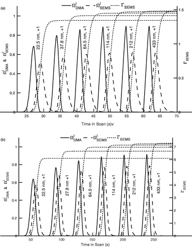
A fast ramp ( = 45 s) accentuates the CPC-induced broadening of the transfer function relative to that of a slow one ( = 240 s), as shown by the instantaneous SEMS transfer function . Moreover, the total number of particles detected during the ramp increases proportionally with the scan time , as indicated by the plateau of the cumulative SEMS transfer function , which by definition represents the overall transmission in the system for particles of given size in an individual scan.

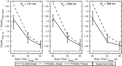
Previous studies have shown substantial differences between the total number of particles detected during up-scans verses down-scans of the same DMA (Collins et al., 2004; Mamakos, Ntziachristos, and Samaras 2008). Figure 7 compares the model predictions of the ratio of the total number of particle counts in an up-scan to that in a down-scan for the three different scanning DMA transfer function models, and as observed experimentally. Three different ramp times, i.e., = 20, 45, 90 s are shown. Only the G-DMA transfer function model shows good agreement with the experimental data. The PFDMA-P transfer function model shows no bias for either up-scan or down-scan operation, so the response ratio based on this transfer function is identical for up- and down-scan operation. While the PFDMA-L transfer function model over-estimates the total concentration in the up-scan over the down-scan by 5% from the experimental data for = 45 and 90 s, the over-estimation exceeds 10% for a 20 s ramp.

Figure 7. Comparison of the experimentally measured and the simulated total number concentration ratios between up- and down-scan operation. Error bars represents the standard deviations for the corresponding experimental measurement results.

3.3. Data inversion

To recover the particle size distribution from the counts recorded in time bins requires solving the inversion problem expressed in Equation (18)(18) for the values of the size distribution at the discretization points . The results presented above reveal the superiority of the transfer function based on the actual DMA geometry (G-DMA) over those obtained using idealized, parallel-flow models of the DMA. Thus, we focus on inversion using the G-DMA model. Most previous SEMS data inversion has built upon the conclusions of Wang and Flagan (1990) that the transfer function for the SEMS is the same as that for the static DMA in the limit of plug flow, provided that the transfer function is evaluated at the mean electric field strength (or voltage) experienced by the particle during its transit through the DMA. The finite time response of the CPC detector is sometimes, but not always, taken into account. Therefore, we also perform the data inversion using the PFDMA-P transfer function. To illustrate the danger of evaluating the transfer function at the voltage applied when particles leave the DMA rather than the transit-mean voltage, we also perform the inversion using the static transfer function.

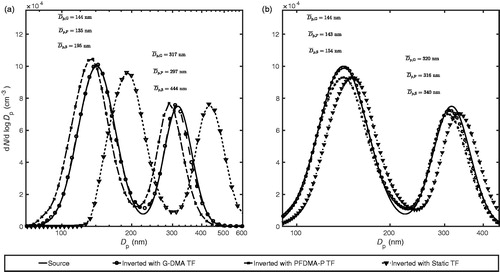
Figure 8 shows the results for an in silico test of these three transfer functions for two bimodal particle size distribution for = (a) 45 s and (b) 240 s scans. The signals have been generated using the G-DMA transfer function. As expected, inversion of the signals using that same G-DMA transfer function yields a size distribution that agrees well with that of the source aerosol. In contrast, the PFDMA-P transfer function underestimates particle size by 7% to 10% in the 45 s ramp, a result of having overestimated the delay time by ∼1 s. The static DMA transfer function produces a much larger bias, overestimating the particle size by 35% to 40% in the 45 s ramp. These biases are reduced in a slow scan (240 s ramp), with PFDMA-P underestimating particle size by about 1%, and static DMA model overestimating particle size by about 6%. We did not compare the PFDMA-L model or other ramp times due to the high computational costs of performing sufficient simulations to fully map the transfer function over the full range of particle sizes.

Figure 8. Comparison of the inverted size distribution with G-DMA model, PFDMA-F model, static DMA transfer function and the source particle size distribution in the (a) 45 s ramp and the (b) 240 s ramp. , and denote the mean particle sizes from G-DMA model, PFDMA-F model, static DMA transfer function-based inversion and for different modes of the size distribution, respectively.

4. Conclusions

This study has examined the integrated SEMS/SMPS instrument using transfer functions for different models of the scanned DMA. Idealized, parallel flow models of the cylindrical DMA assuming either plug flow as considered in the original model of Wang and Flagan (1990) were compared with results obtained using the transfer function for a real DMA, which was obtained from finite element calculations of flow and electric fields within the instrument, and Brownian dynamics simulations of particle migration and transport (Mai and Flagan in press). These scanning DMA models were combined with empirically derived models of the time response of the CPC detector and plumbing between the DMA and CPC. In order to capture the long-time tail of the combined plumbing and detector response, the plug flow plus continuously stirred tank reactor model used in previous studies was augmented with a laminar flow delay time distribution model. The SEMS response function obtained with the geometrical model of the real DMA agrees well with that determined during measurements of monodisperse PSL calibration aerosols that were made with a SEMS/SMPS system consisting of a TSI Model 3081A long-column DMA coupled to a TSI model 3010 CPC as a detector during exponentially increasing voltage up-scans ranging from 10 to 240 s, and during down-scans ranging from 20 to 240 s. Full data inversion was demonstrated with 45 s and 240 s up-scans.

The results presented here reveal biases in the common approach of inverting SEMS data using the constant voltage (DMPS) transfer function in both up-scan and down-scan operation, even when the finite time response of the detector is taken into account; these biases arise because the simplistic model does not accurately describe particle transmission through the scanning DMA. However, very slow scans allow accurate recovery of the size distribution to be obtained by inversion of measured counts using the idealized, parallel-flow DMA transfer function, and can be expected to approach that of properly made DMPS measurements. However, if the transfer function for the actual experimental system is known, the SEMS/SMPS should be able to accurately measure particle size distribution during both up-scans and down-scans.

In the present study, we obtained the real SEMS/SMPS instrument response function using computationally intensive Brownian dynamics simulations for one DMA design, one set of flow rates, one CPC, and a range of scan rates. Rigorous data inversion for other instruments or operating conditions will require that the appropriate scanning-mode transfer function be determined (a costly endeavor) by the method presented here, or the use of scans that are sufficiently slow that the scanning instrument results approach those of DMPS measurements. Alternatively, the SEMS/SMPS instrument response function might be determined empirically by measurement of monodisperse calibration aerosols in a tandem DMA. Ideally, such empirical characterization would involve traceable particle size standards and the use of a well-calibrated reference particle detector that is identical to that used in the SEMS, and with a steady aerosol that can be scanned many times to attain good counting statistics. Because the instrument response function changes when operational parameters change, it needs to be determined for the conditions to be used during measurements. Parameters that need to be reproduced include flow rates, exponential scan time constant, , lengths, sizes, and geometry of all tubing and plumbing connection between the DMA outlet and CPC inlet, counting time, as well as the specific charge conditioner and CPC to be used in the measurements. Because of the sensitivity of the instrument response to details of the instrument, all operating parameters and the instrument response functions need to be well documented.

While the parallel flow models do not fully capture the performance of the scanned DMA, they have been extremely useful in the analysis of DMPS data, particularly using the semi-analytical transfer function that accounts for diffusion (Stolzenburg 1988). It may be possible to develop hybrid models that combine the idealized parallel-flow models with description of the nonidealities that led to their present inclusion in the “extended classification region” of Mai and Flagan (in press). This might incorporate empirically-derived correction factors to account for perturbations to particle transit time, a transmission efficiency for the extended classification region, and a delay time distribution associated with the classification region. With care, the SEMS or SMPS can yield size distributions as faithfully as the DMPS, even in fast scans. However, for data from such approximate descriptions of complex instruments, all of the corrections and approximations to the instrument response function need to be fully and openly documented with each dataset. Raw count data are essential if one is to assess measurement uncertainty.

Many size distributions have been measured with the commercial TSI SMPS and other SEMS systems in the two and a half decades since the method was introduced. Many users have wisely employed relatively slow scans that minimize the perturbations described here, but others have necessarily employed sufficiently fast scans that biases exist in the data. To the extent that the raw data have been preserved, and the operating conditions have been well documented, it may be possible to correct existing data for these biases. To do that will require developing a library of SEMS/SMPS instrument response functions for the range of operating conditions employed. Unfortunately, some data will not be recoverable due to incomplete documentation and preservation of key parameters.

Acknowledgments

The authors thank Dr. K. Beau Farmer of TSI Inc. for providing detailed design drawings of the TSI Model 3081A DMA that made it possible to simulate flows, fields, and particle trajectories in the real instrument. We thank Yuanlong Huang, Wilton Mui, Amanda Grantz, Johannes Leppä, and Paula Popescu for useful discussions.

Disclosure statement

No potential conflict of interest was reported by the authors.

Additional information

Funding

This material is based upon work supported by the National Science Foundation under Grant No. AGS-1602086.

References

- Bracewell, R. N. A. 1986. The Fourier transform and its applications. Vol. 31999. New York: McGraw-Hill.
- Collins, D. R., D. R. Cocker, R. C. Flagan, and J. H. Seinfeld. 2004. The scanning DMA transfer function. Aerosol Sci. Technol. 38 (8):833–50.
- Collins, D. R., R. C. Flagan, and J. H. Seinfeld. 2002. Improved inversion of scanning DMA data. Aerosol Sci. Technol. 36 (1):1–9.
- Dubey, P., and S. Dhaniyala. 2008. Analysis of scanning DMA transfer functions. Aerosol Sci. Technol. 42 (7):544–55.
- Dubey, P., and S. Dhaniyala. 2011. A new approach to calculate diffusional transfer functions of scanning DMAs. Aerosol Sci. Technol. 45 (8):1031–40.
- Hering, S. V., Stolzenburg, M. R., Quant, F. R., Oberreit, D. R., and P. B. Keady. 2005. A Laminar-Flow, Water-Based Condensation Particle Counter (WCPC). Aerosol Sci Technol. 39(7):659–72.
- Knutson, E. O., and K. T. Whitby. 1975. Aerosol classification by electric mobility: Apparatus, theory, and applications. J. Aerosol Sci. 6 (6):443–51.
- Leppä, J., W. Mui, A. M. Grantz, and R. C. Flagan. 2017. Charge distribution uncertainty in differential mobility analysis of aerosols. Aerosol Sci. Technol. 14:1–22.
- Mai, H., and R. C. Flagan. in press. Scanning DMA data analysis I. Classification transfer function. Aerosol Sci. Technol. doi:10.1080/02786826.2018.1528005
- Mamakos, A., L. Ntziachristos, and Z. Samaras. 2008. Differential mobility analyser transfer functions in scanning mode. J. Aerosol Sci. 39 (3):227–43.
- Merritt, M., and Y. Zhang. 2005. Interior-point gradient method for large-scale totally nonnegative least squares problems. J. Optim. Theory Applicat. 126 (1):191–202.
- Quant, F. R., Caldow, R., Sem, G. J., and T. J. Addison. 1992. Performance of Condensation Particle Counters with Three Continuous-Flow Designs. J Aerosol Sci. 23:405–8.
- Russell, L. M., R. C. Flagan, and J. H. Seinfeld. 1995. Asymmetric instrument response resulting from mixing effects in accelerated DMA-CPC measurements. Aerosol Sci. Technol. 23 (4):491–509.
- Stolzenburg, M. R. 1988. An ultrafine aerosol size distribution measuring system. PhD diss., University of Minnesota.
- Wang, S. C., and R. C. Flagan. 1990. Scanning electrical mobility spectrometer. Aerosol Sci. Technol. 13(2):230–240.
- Wang, J., McNeill, V. F., Collins, D. R., and R. C. Flagan. 2002. Fast Mixing Condensation Nucleus Counter: Application to Rapid Scanning Differential Mobility Analyzer Measurements. Aerosol Sci Technol. 36(6):678–89.
- Wolfenbarger, K., and J. H. Seinfeld. 1990. Inversion of aerosol size distribution data. J. Aerosol Sci. 21(2):227–247.