Fine particle mass monitoring with low-cost sensors: Corrections and long-term performance evaluation

Abstract

Low-cost sensors for the measurement of fine particulate matter mass (PM_2.5) enable dense networks to increase the spatial resolution of air quality monitoring. However, these sensors are affected by environmental factors such as temperature and humidity and their effects on ambient aerosol, which must be accounted for to improve the in-field accuracy of these sensors. We conducted long-term tests of two low-cost PM_2.5 sensors: Met-One NPM and PurpleAir PA-II units. We found a high level of self-consistency within each sensor type after testing 25 NPM and 9 PurpleAir units. We developed two types of corrections for the low-cost sensor measurements to better match regulatory-grade data. The first correction accounts for aerosol hygroscopic growth using particle composition and corrects for particle mass below the optical sensor size cut-point by collocation with reference Beta Attenuation Monitors (BAM). A second, fully-empirical correction uses linear or quadratic functions of environmental variables based on the same collocation dataset. The two models yielded comparable improvements over raw measurements. Sensor performance was assessed for two use cases: improving community awareness of air quality with short-term semi-quantitative comparisons of sites and providing long-term reasonably quantitative information for health impact studies. For the short-term case, both sensors provided reasonably accurate concentration information (mean absolute error of ∼4 µg/m³) in near-real time. For the long-term case, tested using year-long collocations at one urban background and one near-source site, error in the annual average was reduced below 1 µg/m³. Hence, these sensors can supplement sparse networks of regulatory-grade instruments, perform high-density neighborhood-scale monitoring, and be used to better understand spatial patterns and temporal air quality trends across urban areas.

Copyright © 2019 American Association for Aerosol Research

1. Introduction

The negative health impacts of exposure to particulate matter (PM) smaller than 2.5 micrometers (PM_2.5) are well documented (e.g., Brook et al. 2010; Pope et al. 2002; Schwartz, Dockery, and Neas 1996). Even relatively small changes in PM_2.5 can have significant impacts on human health and mortality (Lepeule et al. 2012). Reductions in PM_2.5, even in low concentration environments, can have substantial benefits (Apte et al. 2015). Accurate monitoring of PM_2.5 is thus important for a variety of applications, including long-term health studies, assessing the impacts of technology and/or regulatory changes on emissions, and supporting decision-making for future regulatory efforts or to alter individual behavior in real-time. Monitoring is especially of interest in urban areas where the high density of exposed populations is coupled with higher variability in PM due to the large number and variety of sources (Eeftens et al. 2012; Jerrett et al. 2005; Karner, Eisinger, and Niemeier 2010). Thus, a sparse monitoring network can lead to an incomplete understanding of PM_2.5 spatial variability and its subsequent health impacts. Recent advances in low-cost air quality sensing technologies have made it feasible for dense networks of monitors to be deployed in urban areas, providing a neighborhood-scale understanding of air pollution (Snyder et al. 2013). Several pilot programs for monitoring air quality at such high spatial resolution using these technologies are underway (English et al. 2017; Jiao et al. 2016; Williams et al. 2018; Zimmerman et al. 2018).

Most low-cost PM sensors make use of optical measurement techniques (Kelly et al. 2017; Rai et al. 2017; Wang et al. 2015). It is well-known that these optical methods do not generally agree with measurements obtained from instruments operating on different principles (Burkart et al. 2010; Chow et al. 2008; Solomon and Sioutas 2008; Watson et al. 1998; Wilson et al. 2002). For example, work with low-cost optical PM_2.5 sensors (Plantower model PMS3003) showed good correlation (r of 0.8) with a scattered light spectrometer versus low correlation (r of 0.5) with a beta attenuation monitoring (BAM) instrument (Zheng et al. 2018). There are several reasons for these disagreements. First, for regulatory-grade instruments, PM must be reported under specific temperature (20–23 °C) and humidity (30–40%) conditions (US EPA 2016b), while most low-cost sensors report data at ambient conditions, leading to discrepancies with regulatory-grade instruments (including the BAM instruments used in this work, which are recognized as federal equivalent methods for PM_2.5 mass measurement). As ambient humidity increases, hygroscopic growth of particles occurs, which increases their light scattering coefficient (Cabada et al. 2004), and therefore the mass reported by optical sensors. Field testing of low-cost optical PM_2.5 sensors has shown the significant effect of ambient humidity on their measurements (Jayaratne et al. 2018; Zikova, Hopke, and Ferro 2017; Zikova et al. 2017). Accounting for such hygroscopic growth is needed to reduce these humidity effects when comparing the optical sensor to reference monitors. Further, low-cost optical sensors are usually limited to measuring particles larger than 0.3 micrometers (Koehler and Peters 2015; Zhou and Zheng 2016), and so will underreport PM_2.5. This underreporting of small particles by optical PM sensors is corrected for during factory calibration by adjusting the instrument output to match that of a reference PM_2.5 mass measurement of the same calibration “smoke” (Liu et al. 2017). Differences between particle size distribution and composition used for the factory calibration and the ambient aerosol during deployment can therefore cause further errors.

There are currently no established criteria for assessing the performance of low-cost PM sensors (Williams et al. 2019). However, schemes have been proposed with tiered rankings based on relative data quality which recognize that different performance goals may be appropriate for different use cases (e.g., Rai et al. 2017; Williams et al. 2014). For example, while comparison to regulatory standards might require strict criteria (e.g., accuracy ±10%), supplemental monitoring goals including spatial gradient mapping and microenvironment monitoring may have intermediate requirements (±25%) while tracking of sources and distinction of “more polluted” versus “less polluted” areas for public information purposes may have lower requirements (±50%) (Williams et al. 2014, 2019). Another scheme distinguishes between qualitative, semi-quantitative, and reasonably quantitative data (with bias and root mean square deviation below 100%, 50%, and 20%, respectively) suitable for various use cases (Allen 2018). Knowledge of the capabilities and limitations of low-cost sensors with respect to different use cases is especially relevant considering that products such as the PurpleAir sensor are already used by citizen scientists worldwide (www.purpleair.com).

We consider two use cases in this work. First, sensors may be used, e.g., by community monitoring groups, to provide information on local air quality in real-time to support individual decisions, for example about where to go for a walk in a city to avoid highly polluted areas. In this case, the goal is to provide robust indicators, e.g., that PM_2.5 is currently higher in one part of a city than in another, and so less accurate data (even about ±50%) are considered sufficient. Second, sensors may be used to determine long-term trends, e.g., for quantifying the exposure of a population or the impacts of a new pollution-mitigation policy. In this case, more precise long-term performance (relative accuracy of about ±20%) is important. Considering that national average PM_2.5 concentrations in the United States are on the order of 10 µg/m³ (US EPA 2017), we consider measurements with typical error below about 2 µg/m³ to be “reasonably quantitative” data, while higher errors (up to about 5 µg/m³) represent “semi-quantitative” measures (see Section 2.6 for details on the assessment metrics employed).

In this paper, we provide evaluations of the long-term performance of two types of relatively low-cost (under $2000 for the NPM and $250 for the PurpleAir) PM_2.5 sensors in field conditions in the city of Pittsburgh, Pennsylvania and its surroundings. The ambient hourly PM_2.5 concentrations for this study are low (typically below 20 µg/m³) compared to previous field evaluations of these sensors (e.g., Jayaratne et al. 2018; Kelly et al. 2017). We also propose and evaluate both physics-based and fully-empirical methods to correct for the influence of humidity and temperature on sensor readings, thereby making them more comparable to BAM instrument data. We have focused our attention on field studies due to the importance of assessing sensors in a similar environment to that in which they are to be used (Piedrahita et al. 2014; White et al. 2012). In Pittsburgh, like in other urban areas, PM_2.5 is composed of regionally transported (aged) aerosol and fresh vehicular emissions (Tan et al. 2014). Additionally, a metallurgical coke producing facility is a major local point source. Hence, we develop a calibration equation through collocation with a reference monitor at an urban background site that represents aged background PM and a source-oriented site near the major point source. We further evaluate these models across multiple seasons (January 2017 to May 2018) at both locations, as well as at a roadside location where vehicular contribution to PM_2.5 below the sensor size cut-point should be highest, and a more rural location.

2. Methods

2.1. RAMP sensor package and attached PM_2.5 sensors

The Real-time Affordable Multi-Pollutant (RAMP) monitor is a low-cost sensing system collaboratively developed by SenSevere and the Center for Atmospheric Particle Studies at Carnegie Mellon University (Zimmerman et al. 2018). It incorporates five gas sensors, electronics, batteries, and wireless communication hardware. In addition to its internal sensors, the RAMP can be connected to external instruments for measuring PM_2.5. One such instrument is the Met-One Neighborhood Particulate Monitor (NPM) sensor, which uses a forward light scattering laser. The unit is also equipped with an inlet heater and PM_2.5 cyclone. Previous research has assessed the performance of two of these instruments over a two-month period in southern California, and found moderate correlations (r between 0.7 and 0.8) with regulatory-grade instruments (AQ-SPEC 2015). The NPM is available for about $2000 or about one tenth the price of regulatory-grade instruments measuring PM_2.5. A total of 50 NPM units have been deployed alongside RAMPs.

The PurpleAir PM_2.5 monitor (PPA) was also deployed along with the RAMPs. This sensor incorporates a pair of Plantower PMS 5003 laser sensors, which provide measures of PM_2.5 as well as of PM_1.0 and PM₁₀. Previous testing of three of these units over a two-month period in southern California showed good correlation (r above 0.9) with regulatory-grade instruments (AQ-SPEC 2017). This sensor is available for about $250, or about one hundredth of the price of a regulatory-grade instrument. Initial laboratory testing of a batch of 30 PurpleAir units found 7 to be defective; these defects were identified due to low correlations (r < 0.7) between the data provided by each units’ pair of Plantower sensors. These defective sensors are not considered in this paper. A total of 20 PurpleAir units have been deployed with RAMPs in the Pittsburgh area.

2.2. Data collection

Sensor performance was assessed using data collected at four field sites - one corresponding to an “urban background”, one impacted by industrial emissions, one by vehicle emissions, and one more rural site - coincident with monitoring stations operated by the Allegheny County Health Department (ACHD) or Pennsylvania Department of Environmental Protection (DEP), at which BAM instruments provided hourly concentration measurements for comparison (Hacker 2017; McDonnell 2017). Although these instruments are not used for regulatory reporting, they are recognized federal equivalent methods and provide hourly data for Air Quality Index calculations. This section describes the two sites used for correction method development and long-term testing. Two additional regulatory sites which were used to test the correction methods are described in Section 3.3.

The “Lincoln” site (AQS#42-003-7004, 40.308°N by 79.869°W) is a “source-dominated” site within 1 km of a facility producing coke for steel manufacturing that is the largest primary PM_2.5 point source in Allegheny County. This part of Allegheny County exceeded the annual and 24-h Environmental Protection Agency (EPA) PM_2.5 standards over 2015–2017 (ACHD 2017). This site is illustrative of a “fence line” monitoring application, where monitors are placed in proximity to a known emission source. Average PM_2.5 concentration at this site (based on the BAM) was 14.5 µg/m³ in 2017, with a 1-h maximum of 162 µg/m³. Here, one NPM sensor was operated for a total of 294 days from 24 April 2017 until the end of data collection for this study on 1 June 2018. Additionally, between 26 October 2017 and 12 February 2018 (109 days), a total of 12 NPM and 2 PurpleAir sensors were collocated at the site (although not all instruments were active for the entire period).

The “Lawrenceville” deployment site (AQS#42-003-0008, 40.465°N by 79.961°W) is an urban background site located in an urban residential and commercial neighborhood, and part of the EPA’s NCore monitoring network (Hacker 2017). Average PM_2.5 concentration at this site (based on the BAM) was 9.7 µg/m³ in 2017, with a maximum 1-h concentration of 67 µg/m³. At this site, one NPM sensor was operated for a total of 380 days between 13 January 2017 and 6 May 2018. In addition, a total of 25 NPM and 9 PurpleAir sensors were collocated at the site between 30 March 2018 and 4 June 2018 (66 days, although again, not all instruments were present for the entire period). Five NPM sensors were collocated at both Lincoln and Lawrenceville at different times; none of the PurpleAir sensors were collocated at both sites. A deployment timeline is provided in the online Supplemental Information (Figure S2).

Instruments at all sites were connected to RAMP monitors to allow for cellular data transmission. For NPM sensors, data associated with instrument error codes, as well as likely erroneously high readings (exceeding 10,000 µg/m³) were removed from the dataset. For PurpleAir sensors, readings from both internal Plantower sensors were averaged to determine the PurpleAir reading. Measurements from both types of sensors were down-averaged from their collection rate (roughly one measurement every 12 s) to an hourly rate to allow for comparison with the reference instruments.

2.3. Physics-based (hygroscopic growth and size distribution) correction methods

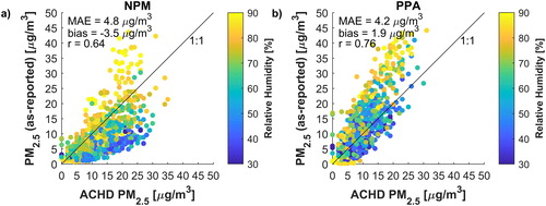
Figure 1 compares the as-reported data from the NPM and PurpleAir sensors to the BAM instrument at the Lawrenceville site. There were sizeable discrepancies (up to 20 µg/m³ in some cases) in the values, with humidity clearly having an effect. A method was sought to correct the readings of the low-cost sensors to better match those of the federal equivalent BAM instruments. As a starting point, the hygroscopic growth factor is the ratio of PM at a given humidity and temperature to that at 22 °C and 35% relative humidity (RH) (the conditions at which regulatory data are reported), and was calculated as follows: (1) $$\mathrm{fRH}\left(T,\mathit{RH}\right)=1+{\mathrm{\kappa }}_{\mathrm{bulk}}\frac{a_w\left(T,\mathit{RH}\right)}{1-a_w\left(T,\mathit{RH}\right)}$$(1)

Figure 1. Comparison of 1-h-average NPM (a) and PurpleAir (b) as-reported sensor readings to the BAM instrument during collocation at the Lawrenceville site. Each point indicates the median across all sensors of the given type present at the site. Shades (colors) indicate RH at the time of the measurements. A breakdown of these results by RH is provided in the online SI (Table S2).

The hygroscopicity of bulk aerosol (${\mathrm{\kappa }}_{\mathrm{bulk}}$) was evaluated considering seasonal changes in particle composition observed in Pittsburgh; these were accounted for by dividing the year into summer (May to September inclusive), winter (November to March inclusive), and other periods (with the “other” period using an average of the summer and winter compositions). Within each period, it was assumed that the aerosol composition and size distribution were constant over time and throughout the urban area. Seasonal aerosol compositions in the Pittsburgh area were obtained from Gu et al. (2018), and literature κ-values for the major non-refractory aerosol components sulfate, nitrate, ammonium, and organic matter were used (Cerully et al. 2015; Petters and Kreidenweis 2007); a sensitivity analysis for this compositional information is provided in the results (Section 3.2) and in the online SI (Section S2). Water activity was calculated as: (2) $$a_w\left(T,\mathit{RH}\right)=\mathit{RH}\exp {\left(\frac{4{\sigma }_w{M}_w}{{\rho }_{w}RT{D}_{\mathrm{p}}}\right)}^{-1}$$(2) where ${\sigma }_w,$ $M_w,$ and ${\rho }_w$ represent the surface tension, molecular weight and density of water, respectively; $T$ is the absolute temperature, $R$ is the ideal gas constant, $\mathit{RH}$ is ambient relative humidity; and $D_{\mathrm{p}}$ is the particle diameter (see online SI, Table S1 for details).

Correction of low-cost sensor readings using the hygroscopic growth factor alone was found to be insufficient (see online SI, Figure S10), likely due to differences between the factory calibration aerosols and ambient aerosol in Pittsburgh. Therefore, the hygroscopic growth correction was combined with an additional linear correction: (3) $$\left[\mathrm{corrected}\mathrm{ }{\mathrm{PM}}_{2.5}\right]={\theta }_1\left(\frac{\left[{\mathrm{PM}}_{2.5}\text{ as reported}\right]}{\mathrm{fRH}\left(T,\mathrm{ }\mathit{RH}\right)}\right)+{\theta }_0$$(3)

The coefficients ${\theta }_0$ and ${\theta }_1$ were estimated using a combination of data collected at both the urban background Lawrenceville and source-dominated Lincoln sites from half of the sensors deployed to each site (the “training” set). Correction model performance was evaluated on the other half of sensors at these sites (the “testing” set), as well as at independent sites (see Section 3.3). Coefficients were set using typical linear regression techniques, minimizing the error between the corrected sensor measurements and the collocated BAM instrument at each site. These coefficients were estimated separately for the different time periods (summer, winter, other) for each of the low-cost sensor types (NPM, PurpleAir). This was necessary to account for the different responses of each type of sensor. For example, seasonal changes in particle size distributions led to changes in the ${\theta }_0$ term as more or less of the PM fell below the 300 nm detection size cut-point for optical sensors.

2.4. Empirical correction methods

The hygroscopic growth factor correction method described above was based on information about the specific aerosol chemical composition of the sensor deployment area, which may not be available at all locations. However, since factors such as temperature and RH are more readily available, other more generalizable, empirical correction equations were developed using these data. Dewpoint ($\mathit{DP})$ was considered as a factor related to condensation that might serve in place of the hygroscopic growth factor; temperature ($T)$ and $\mathit{RH}$ were also considered. Various combinations of the as-reported sensor readings and the above environmental parameters were fit using linear and quadratic regression models to correct the data. The forms of the empirical corrections were selected by trading off performance (across a range of concentrations experienced at both collocation sites) against functional complexity (details are provided in the online SI, Section S3). For NPM sensors, a quadratic function of the sensor reading, temperature, and humidity was selected: (4) $${\left[\mathrm{corrected}\mathrm{ }{\mathrm{PM}}_{2.5}\right]}_{\mathrm{NPM}}={\alpha }_0+{\alpha }_1{\left[{\mathrm{PM}}_{2.5}\right]}_{\mathrm{NPM}}+{\alpha }_{2}T+{\alpha }_{3}RH+{\alpha }_4{\left[{\mathrm{PM}}_{2.5}\right]}_{\mathrm{NPM}}^2+{\alpha }_5{\left[{\mathrm{PM}}_{2.5}\right]}_{\mathrm{NPM}}T+{\alpha }_6{\left[{\mathrm{PM}}_{2.5}\right]}_{\mathrm{NPM}}RH+{\alpha }_7{T}^2+{\mathrm{\alpha }}_{8}T\mathit{RH}+{\alpha }_{9}R{H}^2$$(4)

The form selected for PurpleAir sensors was a two-piece linear function of the sensor reading, T, humidity, and DP, with a threshold at 20 µg/m³: (5) $${\left[\mathrm{corrected}\mathrm{ }{\mathrm{PM}}_{2.5}\right]}_{\mathrm{PPA}}=\left\{\begin{array}{cc}{\beta }_0+{\beta }_1{\left[{\mathrm{PM}}_{2.5}\right]}_{\mathrm{PPA}}+{\beta }_{2}T+{\beta }_{3}RH\mathrm{ }+{\beta }_4\mathrm{D}\mathrm{P}(T,\mathrm{ }\mathit{RH})& \text{if }{\left[{\mathrm{PM}}_{2.5}\right]}_{\mathrm{PPA}}>20\raisebox{1ex}{$\text{µg}$}\!\left/ \!\raisebox{-1ex}{${\mathrm{m}}^3$}\right.\mathrm{ }\\ {\gamma }_0+\mathrm{ }{\gamma }_1{\left[{\mathrm{PM}}_{2.5}\right]}_{\mathrm{PPA}}+{\gamma }_{2}T+{\gamma }_{3}RH\mathrm{ }+\mathrm{ }{\gamma }_4\mathrm{D}\mathrm{P}(T,\mathrm{ }\mathit{RH})& \text{if }{\left[{\mathrm{PM}}_{2.5}\right]}_{\mathrm{PPA}}\le 20\raisebox{1ex}{$\text{μg}$}\!\left/ \!\raisebox{-1ex}{${\mathrm{m}}^3$}\right.\mathrm{ }\end{array}\right.$$(5)

Coefficients calibrated for these equations (using standard regression techniques) along with their uncertainties are provided in the online SI (Table S4).

2.5. In-field drift-adjustment

A seemingly random, non-monotonic fluctuation (e.g., a “random walk”) taking place over a period of weeks or months was observed in field-deployed NPM sensors when Equation (4)(4) $${\left[\mathrm{corrected}\mathrm{ }{\mathrm{PM}}_{2.5}\right]}_{\mathrm{NPM}}={\alpha }_0+{\alpha }_1{\left[{\mathrm{PM}}_{2.5}\right]}_{\mathrm{NPM}}+{\alpha }_{2}T+{\alpha }_{3}RH+{\alpha }_4{\left[{\mathrm{PM}}_{2.5}\right]}_{\mathrm{NPM}}^2+{\alpha }_5{\left[{\mathrm{PM}}_{2.5}\right]}_{\mathrm{NPM}}T+{\alpha }_6{\left[{\mathrm{PM}}_{2.5}\right]}_{\mathrm{NPM}}RH+{\alpha }_7{T}^2+{\mathrm{\alpha }}_{8}T\mathit{RH}+{\alpha }_{9}R{H}^2$$(4) is applied (see online SI, Figure S6). The reason for this was likely due to seasonal changes in aerosol properties and/or sensor behaviors which were not captured by this equation. This was observed to affect monthly average PM_2.5 readings by up to 4 µg/m³ at the Lawrenceville and Lincoln sites. Insufficient data were available to assess whether the same phenomenon occurs for PurpleAir sensors. We propose three methods to adjust for this drift in sensor response over the course of their field deployment. Note that here we use “drift” to refer to any changes in the baseline or “zero” reading of the sensor.

The first adjustment method, known as the “Deployment Records” (DR) method, involved using a log of sensor deployment history to account for biases against a reference instrument. This method involved adjusting the measurements of all sensors to match that of one “benchmark” sensor during periods when sensors were collocated. The benchmark sensor was then collocated with a regulatory-grade instrument while other sensors were deployed in the field. The relative bias of a deployed sensor versus the regulatory-grade instrument was then estimated using the benchmark as an intermediary (i.e., the biases of all sensors versus the benchmark were assessed during their collocations, and the bias of the benchmark versus the regulatory-grade instrument was assessed during its collocation; the bias of any deployed sensor versus the regulatory-grade instrument was then estimated as the sum of the above biases). The second method, known as the “Fifth Percentiles” (5P) method, involved computing the monthly 5P of readings at a given deployment site, and then comparing to the 5P recorded at the nearest regulatory monitoring station. Readings from the deployed sensor were then adjusted so that these percentiles matched. This was done with the assumption that the 5P represented a “background” level to which all sites in the region were subject. The third method was a variation of the 5 P method, known as the “Average of Low readings” (AL) method, which used the average of all readings in a month below 5 µg/m³ as the target value to be matched. All three methods relied on the availability of relatively frequent (e.g., hourly) data from regulatory-grade instruments, and the first method relied on historical collocation data with these instruments. Diagrams depicting each of these proposed methods are provided in the online SI (Figure S7). The latter two methods of rectifying drift by matching distribution parameters over time are similar to those proposed by Tsujita et al. (2005) and used by Moltchanov et al. (2015).

2.6. Assessment metrics

To evaluate the performance of a sensor as compared to a reference (typically a regulatory-grade instrument), the bias, mean absolute error, and correlation coefficient (r) statistics were used (details are provided in the online SI, Section S5). Performance of the instruments was also assessed from a classification perspective, using the EPA’s National Ambient Air Quality Standards 24-h standard of 35 µg/m³ (www.epa.gov/criteria-air-pollutants/naaqs-table) as a representative threshold, by assessing how often the sensor agreed with a reference instrument as to whether this concentration was surpassed. This determination was made on an hourly basis for this assessment, while the regulation cited above applies to daily averages. This comparison was therefore conservative, and we would expect better performance for daily averages based on the results of Section 3.6. Classification precision indicates the fraction of values of concentration $c$ above threshold $\tau$ detected by the sensor which were also detected by the reference: (6) $$\text{classification precision}=\mathrm{ }\frac{{\sum }_{i=1}^n\mathbb{I}\left(c_i>\tau \right)\mathbb{I}\left({\widehat{c}}_i>\tau \right)}{{\sum }_{i=1}^n\mathbb{I}\left(c_i>\tau \right)}·100\mathrm{\%}$$(6) where $c_i$ is the reading of the sensor and ${\widehat{c}}_i$ the reading of the reference instrument at time $i$ of $n,$ and $\mathbb{I}$ is the indicator function, taking on value 1 when its argument is true and 0 otherwise. Classification recall is the fraction of instances detected by the reference instrument which were also detected by the sensor: (7) $$\text{classification recall}=\mathrm{ }\frac{{\sum }_{i=1}^n\mathbb{I}\left(c_i>\tau \right)\mathbb{I}\left({\widehat{c}}_i>\tau \right)}{{\sum }_{i=1}^n\mathbb{I}\left({\widehat{c}}_i>\tau \right)}·100\mathrm{\%}$$(7)

Therefore, classification precision describes how often an event detected by the sensor actually occurred (assuming the reference instrument reading was the “true” concentration) while recall describes the fraction of actual events which were detected by the sensor. Values of these metrics close to 100% indicate better performance.

3. Results

In this section, first, the mutual consistency of the as-reported data from the low-cost PM sensors is quantified, to address how comparisons might be made without applying corrections. Second, the quantitative performance of the proposed correction methods is assessed for the short-term use case envisioned for these sensors. Finally, the long-term performance of these sensors is analyzed, including contributions of the proposed drift-adjustment methods.

3.1. Consistency between sensors

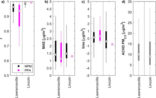
To determine the consistency between sensors, pairwise comparisons of 1-h-averaged data were made among NPM and PurpleAir sensors (i.e., NPM with NPM and PurpleAir with PurpleAir) collocated at either the Lawrenceville or Lincoln site during the same period. At Lawrenceville, during the RAMP collocations, temperature varied between −20 and +31 °C and RH varied from 22% to 97%; at Lincoln, temperature varied from −3 to +43 °C and humidity varied between 17% and 97% (as measured by the RAMPs’ onboard sensors). Figure 2 presents the results of these inter-comparisons; only results for sensors collocated for at least 3 days (72 1-h averages) are presented. Overall, mutual correlations were strong (typically $\mathrm{r}>0.9$) and were higher at the Lincoln site likely due to the wider range of concentrations. Absolute differences in as-reported readings were typically about 2 µg/m³ or less, which includes systematic biases between sensors generally on the order of ±1 µg/m³. This is similar to prior results for Alphasense OPC-N2 optical PM_2.5 sensors, which are more than twice the price of PurpleAir units (Crilley et al. 2018).

Figure 2. Inter-comparison of as-reported 1-h-average data between sensors during collocation periods at both sites. In the boxplots, circles with dots denote the median, thick bars denote the interquartile range, and thin bars denote the 95% confidence range. Black boxplots indicate metric ranges for pairs of NPM sensors, and gray (purple) boxplots indicate ranges for pairs of PurpleAir sensors. This represents 114 NPM pairs at Lawrenceville, 66 NPM pairs at Lincoln, 16 PurpleAir pairs at Lawrenceville and 1 PurpleAir pair at Lincoln. For reference, the ranges of concentrations measured by BAM instruments at the sites during the same time are depicted in (d).

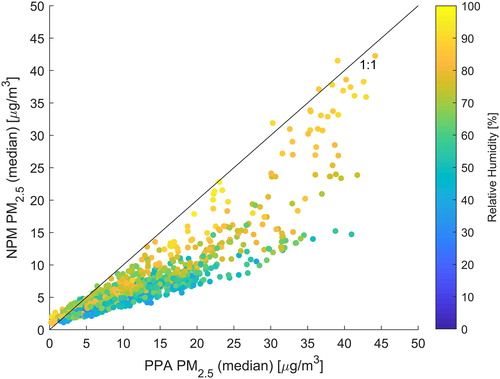
Figure 3 compares hourly averages of as-reported data from NPM sensors at Lawrenceville to those collected by PurpleAir sensors at Lawrenceville as a function of humidity (the median readings of all sensors active at the site at the same time are shown). At low humidity, PurpleAir readings were about twice that of the NPM, while at high humidity the ratio of readings approached one; comparisons made between raw readings of the two sensor types would therefore be heavily humidity-dependent. There are several likely causes for these differences. First, the NPM possesses an inlet heater with a 4-s residence time which activates when RH exceeds 40%. However, this residence time may not be sufficient to totally remove humidity effects on the NPM. Second, these instruments are calibrated differently. The NPM is calibrated with 0.6 µm polystyrene latex spheres (Met One 2018), while PurpleAir Plantowers are calibrated with ambient aerosol across several cities in China (Wang 2019). They therefore respond differently when exposed to a common aerosol which differs from their calibration aerosols.

Figure 3. Comparison between medians of as-reported 1-h-average data of 25 NPM and 9 PurpleAir sensors during collocation at the Lawrenceville site. Shades (colors) indicate RH at the time of the measurements.

3.2. Correction of low-cost sensors towards a federal equivalent method

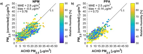
Figure 4 plots median hourly-average readings from NPM and PurpleAir sensors collocated at the Lawrenceville site corrected using Equation (3)(3) $$\left[\mathrm{corrected}\mathrm{ }{\mathrm{PM}}_{2.5}\right]={\theta }_1\left(\frac{\left[{\mathrm{PM}}_{2.5}\text{ as reported}\right]}{\mathrm{fRH}\left(T,\mathrm{ }\mathit{RH}\right)}\right)+{\theta }_0$$(3) against the ACHD regulatory-grade (BAM) instrument readings. This correction decreased MAE by about 40% for both NPM and PurpleAir sensors with respect to their as-reported values and reduced bias significantly, but there was still noticeable measurement noise (r ∼0.75) about the identity line.

Figure 4. Comparison of 1-h-average NPM (a) and PurpleAir (b) sensor readings to the BAM instrument during collocation at the Lawrenceville site after correction using Equation (3)(3) $$\left[\mathrm{corrected}\mathrm{ }{\mathrm{PM}}_{2.5}\right]={\theta }_1\left(\frac{\left[{\mathrm{PM}}_{2.5}\text{ as reported}\right]}{\mathrm{fRH}\left(T,\mathrm{ }\mathit{RH}\right)}\right)+{\theta }_0$$(3) , with appropriate coefficients for NPM and PurpleAir. Each point indicates the median across all sensors of the given type present at the site (including both “training” and “testing” sensors). Shades (colors) indicate RH at the time of the measurements. A breakdown of these results by RH is provided in the online SI (Table S3).

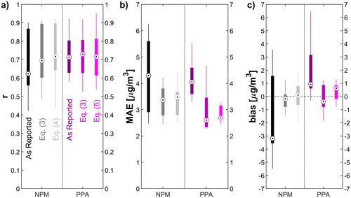
Figure 5 assesses the performance of the designated “testing” set of low-cost sensors deployed to the Lawrenceville and Lincoln sites during the March to June (at Lawrenceville) and October to February (at Lincoln) collocation periods. The figure compares as-reported data to data corrected using the hygroscopic-growth-based approach of Equation (3)(3) $$\left[\mathrm{corrected}\mathrm{ }{\mathrm{PM}}_{2.5}\right]={\theta }_1\left(\frac{\left[{\mathrm{PM}}_{2.5}\text{ as reported}\right]}{\mathrm{fRH}\left(T,\mathrm{ }\mathit{RH}\right)}\right)+{\theta }_0$$(3) (with appropriate coefficients for NPM or PurpleAir sensors) and data corrected using the fully-empirical approaches of Equation (4)(4) $${\left[\mathrm{corrected}\mathrm{ }{\mathrm{PM}}_{2.5}\right]}_{\mathrm{NPM}}={\alpha }_0+{\alpha }_1{\left[{\mathrm{PM}}_{2.5}\right]}_{\mathrm{NPM}}+{\alpha }_{2}T+{\alpha }_{3}RH+{\alpha }_4{\left[{\mathrm{PM}}_{2.5}\right]}_{\mathrm{NPM}}^2+{\alpha }_5{\left[{\mathrm{PM}}_{2.5}\right]}_{\mathrm{NPM}}T+{\alpha }_6{\left[{\mathrm{PM}}_{2.5}\right]}_{\mathrm{NPM}}RH+{\alpha }_7{T}^2+{\mathrm{\alpha }}_{8}T\mathit{RH}+{\alpha }_{9}R{H}^2$$(4) for NPM or Equation (5)(5) $${\left[\mathrm{corrected}\mathrm{ }{\mathrm{PM}}_{2.5}\right]}_{\mathrm{PPA}}=\left\{\begin{array}{cc}{\beta }_0+{\beta }_1{\left[{\mathrm{PM}}_{2.5}\right]}_{\mathrm{PPA}}+{\beta }_{2}T+{\beta }_{3}RH\mathrm{ }+{\beta }_4\mathrm{D}\mathrm{P}(T,\mathrm{ }\mathit{RH})& \text{if }{\left[{\mathrm{PM}}_{2.5}\right]}_{\mathrm{PPA}}>20\raisebox{1ex}{$\text{µg}$}\!\left/ \!\raisebox{-1ex}{${\mathrm{m}}^3$}\right.\mathrm{ }\\ {\gamma }_0+\mathrm{ }{\gamma }_1{\left[{\mathrm{PM}}_{2.5}\right]}_{\mathrm{PPA}}+{\gamma }_{2}T+{\gamma }_{3}RH\mathrm{ }+\mathrm{ }{\gamma }_4\mathrm{D}\mathrm{P}(T,\mathrm{ }\mathit{RH})& \text{if }{\left[{\mathrm{PM}}_{2.5}\right]}_{\mathrm{PPA}}\le 20\raisebox{1ex}{$\text{μg}$}\!\left/ \!\raisebox{-1ex}{${\mathrm{m}}^3$}\right.\mathrm{ }\end{array}\right.$$(5) for PurpleAir. In all cases hourly-averaged data were used. In terms of correlation (Figure 5a), no improvement was made for PurpleAir sensors, while only a modest improvement resulted from correction of the NPM sensors. In terms of MAE (Figure 5b) and bias (Figure 5c), however, both correction approaches resulted in noticeable improvements. For NPM sensors, both the physics-based Equation (3)(3) $$\left[\mathrm{corrected}\mathrm{ }{\mathrm{PM}}_{2.5}\right]={\theta }_1\left(\frac{\left[{\mathrm{PM}}_{2.5}\text{ as reported}\right]}{\mathrm{fRH}\left(T,\mathrm{ }\mathit{RH}\right)}\right)+{\theta }_0$$(3) and fully-empirical Equation (4)(4) $${\left[\mathrm{corrected}\mathrm{ }{\mathrm{PM}}_{2.5}\right]}_{\mathrm{NPM}}={\alpha }_0+{\alpha }_1{\left[{\mathrm{PM}}_{2.5}\right]}_{\mathrm{NPM}}+{\alpha }_{2}T+{\alpha }_{3}RH+{\alpha }_4{\left[{\mathrm{PM}}_{2.5}\right]}_{\mathrm{NPM}}^2+{\alpha }_5{\left[{\mathrm{PM}}_{2.5}\right]}_{\mathrm{NPM}}T+{\alpha }_6{\left[{\mathrm{PM}}_{2.5}\right]}_{\mathrm{NPM}}RH+{\alpha }_7{T}^2+{\mathrm{\alpha }}_{8}T\mathit{RH}+{\alpha }_{9}R{H}^2$$(4) gave comparable performance. For PurpleAir sensors, the fully-empirical approach of Equation (5)(5) $${\left[\mathrm{corrected}\mathrm{ }{\mathrm{PM}}_{2.5}\right]}_{\mathrm{PPA}}=\left\{\begin{array}{cc}{\beta }_0+{\beta }_1{\left[{\mathrm{PM}}_{2.5}\right]}_{\mathrm{PPA}}+{\beta }_{2}T+{\beta }_{3}RH\mathrm{ }+{\beta }_4\mathrm{D}\mathrm{P}(T,\mathrm{ }\mathit{RH})& \text{if }{\left[{\mathrm{PM}}_{2.5}\right]}_{\mathrm{PPA}}>20\raisebox{1ex}{$\text{µg}$}\!\left/ \!\raisebox{-1ex}{${\mathrm{m}}^3$}\right.\mathrm{ }\\ {\gamma }_0+\mathrm{ }{\gamma }_1{\left[{\mathrm{PM}}_{2.5}\right]}_{\mathrm{PPA}}+{\gamma }_{2}T+{\gamma }_{3}RH\mathrm{ }+\mathrm{ }{\gamma }_4\mathrm{D}\mathrm{P}(T,\mathrm{ }\mathit{RH})& \text{if }{\left[{\mathrm{PM}}_{2.5}\right]}_{\mathrm{PPA}}\le 20\raisebox{1ex}{$\text{μg}$}\!\left/ \!\raisebox{-1ex}{${\mathrm{m}}^3$}\right.\mathrm{ }\end{array}\right.$$(5) provided a smaller spread of MAE and bias results as compared to Equation (3)(3) $$\left[\mathrm{corrected}\mathrm{ }{\mathrm{PM}}_{2.5}\right]={\theta }_1\left(\frac{\left[{\mathrm{PM}}_{2.5}\text{ as reported}\right]}{\mathrm{fRH}\left(T,\mathrm{ }\mathit{RH}\right)}\right)+{\theta }_0$$(3) , while the median MAE of both approaches were almost the same, and the median bias of Equation (5)(5) $${\left[\mathrm{corrected}\mathrm{ }{\mathrm{PM}}_{2.5}\right]}_{\mathrm{PPA}}=\left\{\begin{array}{cc}{\beta }_0+{\beta }_1{\left[{\mathrm{PM}}_{2.5}\right]}_{\mathrm{PPA}}+{\beta }_{2}T+{\beta }_{3}RH\mathrm{ }+{\beta }_4\mathrm{D}\mathrm{P}(T,\mathrm{ }\mathit{RH})& \text{if }{\left[{\mathrm{PM}}_{2.5}\right]}_{\mathrm{PPA}}>20\raisebox{1ex}{$\text{µg}$}\!\left/ \!\raisebox{-1ex}{${\mathrm{m}}^3$}\right.\mathrm{ }\\ {\gamma }_0+\mathrm{ }{\gamma }_1{\left[{\mathrm{PM}}_{2.5}\right]}_{\mathrm{PPA}}+{\gamma }_{2}T+{\gamma }_{3}RH\mathrm{ }+\mathrm{ }{\gamma }_4\mathrm{D}\mathrm{P}(T,\mathrm{ }\mathit{RH})& \text{if }{\left[{\mathrm{PM}}_{2.5}\right]}_{\mathrm{PPA}}\le 20\raisebox{1ex}{$\text{μg}$}\!\left/ \!\raisebox{-1ex}{${\mathrm{m}}^3$}\right.\mathrm{ }\end{array}\right.$$(5) was slightly worse. Overall both correction approaches improved upon the as-reported data and there was no significant difference between their performances.

Figure 5. Performance metrics of 1-h-average as-reported and corrected sensor data compared to BAM instruments during collocation at both the Lawrenceville and Lincoln sites. Results shown relate to a total of 17 NPM and 5 PurpleAir sensors of the “testing” set. Corrections are performed using either the approach of Equation (3)(3) $$\left[\mathrm{corrected}\mathrm{ }{\mathrm{PM}}_{2.5}\right]={\theta }_1\left(\frac{\left[{\mathrm{PM}}_{2.5}\text{ as reported}\right]}{\mathrm{fRH}\left(T,\mathrm{ }\mathit{RH}\right)}\right)+{\theta }_0$$(3) , with appropriate coefficients for NPM or PurpleAir, or the approaches of Equation (4)(4) $${\left[\mathrm{corrected}\mathrm{ }{\mathrm{PM}}_{2.5}\right]}_{\mathrm{NPM}}={\alpha }_0+{\alpha }_1{\left[{\mathrm{PM}}_{2.5}\right]}_{\mathrm{NPM}}+{\alpha }_{2}T+{\alpha }_{3}RH+{\alpha }_4{\left[{\mathrm{PM}}_{2.5}\right]}_{\mathrm{NPM}}^2+{\alpha }_5{\left[{\mathrm{PM}}_{2.5}\right]}_{\mathrm{NPM}}T+{\alpha }_6{\left[{\mathrm{PM}}_{2.5}\right]}_{\mathrm{NPM}}RH+{\alpha }_7{T}^2+{\mathrm{\alpha }}_{8}T\mathit{RH}+{\alpha }_{9}R{H}^2$$(4) for NPM and Equation (5)(5) $${\left[\mathrm{corrected}\mathrm{ }{\mathrm{PM}}_{2.5}\right]}_{\mathrm{PPA}}=\left\{\begin{array}{cc}{\beta }_0+{\beta }_1{\left[{\mathrm{PM}}_{2.5}\right]}_{\mathrm{PPA}}+{\beta }_{2}T+{\beta }_{3}RH\mathrm{ }+{\beta }_4\mathrm{D}\mathrm{P}(T,\mathrm{ }\mathit{RH})& \text{if }{\left[{\mathrm{PM}}_{2.5}\right]}_{\mathrm{PPA}}>20\raisebox{1ex}{$\text{µg}$}\!\left/ \!\raisebox{-1ex}{${\mathrm{m}}^3$}\right.\mathrm{ }\\ {\gamma }_0+\mathrm{ }{\gamma }_1{\left[{\mathrm{PM}}_{2.5}\right]}_{\mathrm{PPA}}+{\gamma }_{2}T+{\gamma }_{3}RH\mathrm{ }+\mathrm{ }{\gamma }_4\mathrm{D}\mathrm{P}(T,\mathrm{ }\mathit{RH})& \text{if }{\left[{\mathrm{PM}}_{2.5}\right]}_{\mathrm{PPA}}\le 20\raisebox{1ex}{$\text{μg}$}\!\left/ \!\raisebox{-1ex}{${\mathrm{m}}^3$}\right.\mathrm{ }\end{array}\right.$$(5) for PurpleAir.

Table 1 presents the calibrated coefficients for the approach of Equation (3)(3) $$\left[\mathrm{corrected}\mathrm{ }{\mathrm{PM}}_{2.5}\right]={\theta }_1\left(\frac{\left[{\mathrm{PM}}_{2.5}\text{ as reported}\right]}{\mathrm{fRH}\left(T,\mathrm{ }\mathit{RH}\right)}\right)+{\theta }_0$$(3) for both NPM and PurpleAir sensors during the summer, winter, and for other periods (calibrated coefficients for Equations (4)(4) $${\left[\mathrm{corrected}\mathrm{ }{\mathrm{PM}}_{2.5}\right]}_{\mathrm{NPM}}={\alpha }_0+{\alpha }_1{\left[{\mathrm{PM}}_{2.5}\right]}_{\mathrm{NPM}}+{\alpha }_{2}T+{\alpha }_{3}RH+{\alpha }_4{\left[{\mathrm{PM}}_{2.5}\right]}_{\mathrm{NPM}}^2+{\alpha }_5{\left[{\mathrm{PM}}_{2.5}\right]}_{\mathrm{NPM}}T+{\alpha }_6{\left[{\mathrm{PM}}_{2.5}\right]}_{\mathrm{NPM}}RH+{\alpha }_7{T}^2+{\mathrm{\alpha }}_{8}T\mathit{RH}+{\alpha }_{9}R{H}^2$$(4) and (5)(5) $${\left[\mathrm{corrected}\mathrm{ }{\mathrm{PM}}_{2.5}\right]}_{\mathrm{PPA}}=\left\{\begin{array}{cc}{\beta }_0+{\beta }_1{\left[{\mathrm{PM}}_{2.5}\right]}_{\mathrm{PPA}}+{\beta }_{2}T+{\beta }_{3}RH\mathrm{ }+{\beta }_4\mathrm{D}\mathrm{P}(T,\mathrm{ }\mathit{RH})& \text{if }{\left[{\mathrm{PM}}_{2.5}\right]}_{\mathrm{PPA}}>20\raisebox{1ex}{$\text{µg}$}\!\left/ \!\raisebox{-1ex}{${\mathrm{m}}^3$}\right.\mathrm{ }\\ {\gamma }_0+\mathrm{ }{\gamma }_1{\left[{\mathrm{PM}}_{2.5}\right]}_{\mathrm{PPA}}+{\gamma }_{2}T+{\gamma }_{3}RH\mathrm{ }+\mathrm{ }{\gamma }_4\mathrm{D}\mathrm{P}(T,\mathrm{ }\mathit{RH})& \text{if }{\left[{\mathrm{PM}}_{2.5}\right]}_{\mathrm{PPA}}\le 20\raisebox{1ex}{$\text{μg}$}\!\left/ \!\raisebox{-1ex}{${\mathrm{m}}^3$}\right.\mathrm{ }\end{array}\right.$$(5) are provided in the online SI, Table S4). Note that for both NPM and PurpleAir sensors, the value of ${\theta }_0$ (the linear intercept term) was larger in summer than in winter. This could be explained by the fact that during summertime in Pittsburgh, as in most urban areas (Asmi et al. 2011), particles smaller than 300 nm optical diameter are a larger fraction of PM_2.5 (see the online SI, Figure S9), necessitating a larger correction. For ${\theta }_1$ (the linear slope term), while the values for summer and winter were the same for NPM sensors, for PurpleAir sensors the value was higher in the winter. However, the hygroscopic growth factor (for the same temperature and RH) was also higher in winter, as winter-time aerosol has a larger contribution from more hygroscopic inorganic aerosol. Thus, the net result was a lower impact of seasonal changes in the hygroscopic growth factor on the PurpleAir readings, indicating that the PurpleAir sensor may be less susceptible to humidity-driven changes. The internal structure of the PurpleAir unit may contribute to this; the plastic shell enclosing the Plantower sensors and associated electronic circuits can trap heat inside the unit, leading to lower RH within the device. During tests at the Lawrenceville site, $\mathit{RH}$ inside the PurpleAir was found to be 9.7 percentage points lower on average than outside, while $T$ was 2.7 °C higher.

Table 1. Calibrated coefficients for Equation (3)(3) $$\left[\mathrm{corrected}\mathrm{ }{\mathrm{PM}}_{2.5}\right]={\theta }_1\left(\frac{\left[{\mathrm{PM}}_{2.5}\text{ as reported}\right]}{\mathrm{fRH}\left(T,\mathrm{ }\mathit{RH}\right)}\right)+{\theta }_0$$(3) . Values following “$\pm$” represent the standard deviations in the coefficient estimates.

		Met-One NPM		PurpleAir PPA
${\theta }_0$	Summer	$5.28\pm 0.09$	$\raisebox{1ex}{$\text{μg}$}\!\left/ \!\raisebox{-1ex}{${\mathrm{m}}^3$}\right.$	$5.4\pm 0.4$	$\raisebox{1ex}{$\text{μg}$}\!\left/ \!\raisebox{-1ex}{${\mathrm{m}}^3$}\right.$
	Winter	$2.03\pm 0.08$	$\raisebox{1ex}{$\text{μg}$}\!\left/ \!\raisebox{-1ex}{${\mathrm{m}}^3$}\right.$	$-0.3\pm 0.2$	$\raisebox{1ex}{$\text{μg}$}\!\left/ \!\raisebox{-1ex}{${\mathrm{m}}^3$}\right.$
	Other	$1.68\pm 0.13$	$\raisebox{1ex}{$\text{μg}$}\!\left/ \!\raisebox{-1ex}{${\mathrm{m}}^3$}\right.$	$3.7\pm 0.1$	$\raisebox{1ex}{$\text{μg}$}\!\left/ \!\raisebox{-1ex}{${\mathrm{m}}^3$}\right.$
${\theta }_1$	Summer	$1.50\pm 0.01$		$0.62\pm 0.03$
	Winter	$1.50\pm 0.01$		$1.25\pm 0.01$
	Other	$1.76\pm 0.02$		$0.83\pm 0.01$

3.3. Performance assessment at other regulatory sites

To further assess the performance of these sensor corrections at locations independent of where they were developed, several sensors were tested at two additional sites. The “Parkway East” site (AQS#42-003-1376, 40.437°N by 79.864°W) represents a roadside location (Hacker 2017), and thus may have a different, vehicular traffic-influenced particle composition and size distribution than either the urban background or coke oven-impacted sites at which the corrections were developed. Between 6 and 27 September 2018 (21 days), two PurpleAir sensors were collocated at this site. Data from these sensors were corrected using Equation (3)(3) $$\left[\mathrm{corrected}\mathrm{ }{\mathrm{PM}}_{2.5}\right]={\theta }_1\left(\frac{\left[{\mathrm{PM}}_{2.5}\text{ as reported}\right]}{\mathrm{fRH}\left(T,\mathrm{ }\mathit{RH}\right)}\right)+{\theta }_0$$(3) . These provided comparable results to testing at the Lincoln and Lawrenceville sites (median r of 0.71, median MAE of 2.7 µg/m³, median bias of 0.36 µg/m³). For reference, the average concentration at this site during the same time was 10.6 µg/m³.

The “DEP Johnstown” site (AQS#42-021-0011, 40.310°N by 78.915°W) is in Cambria county, about 90 kilometers east of Pittsburgh (McDonnell 2017). While possessing a similar overall climate to Pittsburgh, it represents a more rural site. From 3 to 6 April 2017 (3 days), a single NPM sensor was deployed at this site. Data from this sensor was corrected using Equation (3)(3) $$\left[\mathrm{corrected}\mathrm{ }{\mathrm{PM}}_{2.5}\right]={\theta }_1\left(\frac{\left[{\mathrm{PM}}_{2.5}\text{ as reported}\right]}{\mathrm{fRH}\left(T,\mathrm{ }\mathit{RH}\right)}\right)+{\theta }_0$$(3) , and gave performance within the ranges observed at the other sites (r of 0.62, MAE of 1.9 µg/m³, bias of −0.99 µg/m³). For reference, the average concentration at this site during the same time was 6.2 µg/m³.

3.4. Sensitivity analysis to aerosol composition

Since hygroscopic growth is composition dependent (Petters and Kreidenweis 2007), different aerosol compositions may experience different rates of growth. While the hygroscopic growth correction method discussed earlier used aerosol composition data from Aerosol Mass Spectrometer (AMS) measurements, not all locations have such data. However, aerosol composition data is also collected on a regular basis (one 24-h sample every three to six days) by regulatory agencies such as the US EPA, and the data are publicly available (https://aqs.epa.gov/aqsweb/airdata/download_files.html). For example, aerosol composition data from Washington County, a site 35 kilometers from Pittsburgh, was used as a proxy for Pittsburgh aerosol composition; this resulted in a difference of less than 1% in the corrected PM_2.5 concentration values. A sensitivity analysis for the hygroscopic-growth-based correction approach with respect to aerosol composition was also performed using a range of plausible compositions from the EPA Chemical Speciation Network (US EPA 2019). Full details are provided in the online SI (Section S2). Briefly, the organic component fraction varied from 0.3 to 1, the sulfate component varied from 0 to 0.8, nitrate varied from 0 to 0.8, and ammonium varied from 0 to 0.3. Overall, using this range of alternate chemical composition information in Equation (3)(3) $$\left[\mathrm{corrected}\mathrm{ }{\mathrm{PM}}_{2.5}\right]={\theta }_1\left(\frac{\left[{\mathrm{PM}}_{2.5}\text{ as reported}\right]}{\mathrm{fRH}\left(T,\mathrm{ }\mathit{RH}\right)}\right)+{\theta }_0$$(3) changed the resulting corrected PM_2.5 concentrations by up to 10% for typical cases, and up to 25% in extreme cases (see online SI, Figure S5). Thus, for US sites where no local composition information is available, publicly-available information from the nearest site in the EPA network can be used. A similar approach may be possible for other countries.

3.5. Short-term performance

The US EPA has a short-term standard for PM_2.5 based on 24-h average concentrations, set at 35 µg/m³ (US EPA 2016a). We use this concentration level to test the performance of these low-cost sensors under a short-term use case, where they might be used to alert citizens to potentially unhealthy outdoor conditions. Although the EPA standard applies to a 24-h average concentration, we test the performance of the low-cost sensors using 1-h averages in order to better mimic a near real-time alert scenario. This test is performed for the Lincoln site only since hourly concentrations at Lawrenceville surpassed the threshold less than 1% of the time. True positives occurred when both the NPM sensor (corrected using Equation (3)(3) $$\left[\mathrm{corrected}\mathrm{ }{\mathrm{PM}}_{2.5}\right]={\theta }_1\left(\frac{\left[{\mathrm{PM}}_{2.5}\text{ as reported}\right]}{\mathrm{fRH}\left(T,\mathrm{ }\mathit{RH}\right)}\right)+{\theta }_0$$(3) ) and BAM detected an event (i.e., an hour when the average PM_2.5 concentration was higher than 35 µg/m³); false positives were when only the NPM measured the event, and false negatives when the NPM failed to detect an event seen by the BAM. The classification precision (Equation (6)(6) $$\text{classification precision}=\mathrm{ }\frac{{\sum }_{i=1}^n\mathbb{I}\left(c_i>\tau \right)\mathbb{I}\left({\widehat{c}}_i>\tau \right)}{{\sum }_{i=1}^n\mathbb{I}\left(c_i>\tau \right)}·100\mathrm{\%}$$(6) ) of the sensor was 85% and its classification recall (Equation (7)(7) $$\text{classification recall}=\mathrm{ }\frac{{\sum }_{i=1}^n\mathbb{I}\left(c_i>\tau \right)\mathbb{I}\left({\widehat{c}}_i>\tau \right)}{{\sum }_{i=1}^n\mathbb{I}\left({\widehat{c}}_i>\tau \right)}·100\mathrm{\%}$$(7) ) was 71% at the Lincoln site; for comparison, these values were 61% and 78% respectively for the un-corrected, as-reported NPM data. Of the misclassifications, 15% occurred when the BAM measured average concentrations between 30 and 40 µg/m³; the rest represented larger discrepancies between the instruments. A 1 h “grace period” was also considered, i.e., if an event detection by one instrument leads or trails the other by up to an hour, this was still counted as a true positive. With this grace period, the classification precision was 90% and classification recall was 97%, versus 73% and 97% respectively for the uncorrected data. A graphical presentation of the results is provided in the online SI (Figure S16).

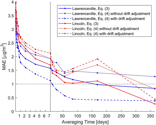
3.6. Long-term performance

Long-term assessment is necessary to categorize bias and assess data quality after extensive field use of sensors. Additionally, long-term deployments can be used to generate data for epidemiological studies, to evaluate different air quality models, and for verification of satellite retrievals, which rely on sparse networks of expensive reference monitors. Previous studies of lower-cost optical particle counters operating for up to four months report no evidence of significant drift (Crilley et al. 2018). The long-term performance of NPM sensors was assessed using data collected by the two sensors deployed at the Lawrenceville and Lincoln sites for a much more extended period (e.g., more than a year of data at Lawrenceville collected over a 16-month span). First, data corrected using Equation (4)(4) $${\left[\mathrm{corrected}\mathrm{ }{\mathrm{PM}}_{2.5}\right]}_{\mathrm{NPM}}={\alpha }_0+{\alpha }_1{\left[{\mathrm{PM}}_{2.5}\right]}_{\mathrm{NPM}}+{\alpha }_{2}T+{\alpha }_{3}RH+{\alpha }_4{\left[{\mathrm{PM}}_{2.5}\right]}_{\mathrm{NPM}}^2+{\alpha }_5{\left[{\mathrm{PM}}_{2.5}\right]}_{\mathrm{NPM}}T+{\alpha }_6{\left[{\mathrm{PM}}_{2.5}\right]}_{\mathrm{NPM}}RH+{\alpha }_7{T}^2+{\mathrm{\alpha }}_{8}T\mathit{RH}+{\alpha }_{9}R{H}^2$$(4) were used to assess the in-field drift-adjustment methods proposed in Section 2.5 to eliminate the “random walk” behavior observed when this correction approach was used over long periods. Based on these results, the “average of low readings” method worked best, reducing both the median bias and spread in biases at the Lawrenceville site. However, there were no clear improvements for these metrics at the Lincoln site (see online SI, Figure S8).

Figure 6 plots the MAE of the corrected sensor data with and without drift-adjustment (using the AL method) compared to the associated regulatory-grade instrument, as a function of averaging period. For weekly averages error was below about 2 µg/m³. For annual averages, errors were about or below 1 µg/m³, which is about 10% of the annual average concentrations for Pittsburgh. Drift-adjustment of measurements corrected with the fully-empirical Equation (4)(4) $${\left[\mathrm{corrected}\mathrm{ }{\mathrm{PM}}_{2.5}\right]}_{\mathrm{NPM}}={\alpha }_0+{\alpha }_1{\left[{\mathrm{PM}}_{2.5}\right]}_{\mathrm{NPM}}+{\alpha }_{2}T+{\alpha }_{3}RH+{\alpha }_4{\left[{\mathrm{PM}}_{2.5}\right]}_{\mathrm{NPM}}^2+{\alpha }_5{\left[{\mathrm{PM}}_{2.5}\right]}_{\mathrm{NPM}}T+{\alpha }_6{\left[{\mathrm{PM}}_{2.5}\right]}_{\mathrm{NPM}}RH+{\alpha }_7{T}^2+{\mathrm{\alpha }}_{8}T\mathit{RH}+{\alpha }_{9}R{H}^2$$(4) improved the performance at the Lawrenceville site (where concentrations are typically lower) to exceed that of Equation (3)(3) $$\left[\mathrm{corrected}\mathrm{ }{\mathrm{PM}}_{2.5}\right]={\theta }_1\left(\frac{\left[{\mathrm{PM}}_{2.5}\text{ as reported}\right]}{\mathrm{fRH}\left(T,\mathrm{ }\mathit{RH}\right)}\right)+{\theta }_0$$(3) ; here, the errors fall below 1 µg/m³ for quarterly or seasonal averages. At the Lincoln site the drift-adjustment method tended to do nothing, or to slightly increase errors; this indicates that drift adjustment may not be required (or even suitable) for all locations or all sensors.

Figure 6. Mean absolute error in PM_2.5 measurements for two NPM sensors during long-term deployments as a function of averaging period (note the differing horizontal axis scale on either side of the vertical black line). Solid lines represent measurements corrected using Equation (3)(3) $$\left[\mathrm{corrected}\mathrm{ }{\mathrm{PM}}_{2.5}\right]={\theta }_1\left(\frac{\left[{\mathrm{PM}}_{2.5}\text{ as reported}\right]}{\mathrm{fRH}\left(T,\mathrm{ }\mathit{RH}\right)}\right)+{\theta }_0$$(3) ; dotted lines indicate measures corrected using Equation (4)(4) $${\left[\mathrm{corrected}\mathrm{ }{\mathrm{PM}}_{2.5}\right]}_{\mathrm{NPM}}={\alpha }_0+{\alpha }_1{\left[{\mathrm{PM}}_{2.5}\right]}_{\mathrm{NPM}}+{\alpha }_{2}T+{\alpha }_{3}RH+{\alpha }_4{\left[{\mathrm{PM}}_{2.5}\right]}_{\mathrm{NPM}}^2+{\alpha }_5{\left[{\mathrm{PM}}_{2.5}\right]}_{\mathrm{NPM}}T+{\alpha }_6{\left[{\mathrm{PM}}_{2.5}\right]}_{\mathrm{NPM}}RH+{\alpha }_7{T}^2+{\mathrm{\alpha }}_{8}T\mathit{RH}+{\alpha }_{9}R{H}^2$$(4) but not drift-adjusted; dashed lines indicate measures corrected using Equation (4)(4) $${\left[\mathrm{corrected}\mathrm{ }{\mathrm{PM}}_{2.5}\right]}_{\mathrm{NPM}}={\alpha }_0+{\alpha }_1{\left[{\mathrm{PM}}_{2.5}\right]}_{\mathrm{NPM}}+{\alpha }_{2}T+{\alpha }_{3}RH+{\alpha }_4{\left[{\mathrm{PM}}_{2.5}\right]}_{\mathrm{NPM}}^2+{\alpha }_5{\left[{\mathrm{PM}}_{2.5}\right]}_{\mathrm{NPM}}T+{\alpha }_6{\left[{\mathrm{PM}}_{2.5}\right]}_{\mathrm{NPM}}RH+{\alpha }_7{T}^2+{\mathrm{\alpha }}_{8}T\mathit{RH}+{\alpha }_{9}R{H}^2$$(4) and drift-adjusted using the AL method. Points along the lines indicate which specific averaging times were evaluated.

4. Discussion

Testing of a relatively large number of NPM (25 sensors at the Lawrenceville site) and PurpleAir (9 sensors at the Lawrenceville site) low-cost PM_2.5 sensors showed high mutual consistency between the sensors, with mean inter-unit disagreement typically below 2.5 µg/m³ and correlation typically higher than 0.9. Systematic biases between instruments appear to account for the largest fraction of the absolute differences; such biases may be assessed before and after field deployment using collocations, but this may not fully account for in-field differences due to changes in aerosol composition, size distributions, and electronic sensor performance variability over time (see online SI, Section S2).

The first proposed correction equation was designed to account for two of the main factors contributing to differences between optical measurements and the BAM instrument readings (which report PM_2.5 mass at a fixed temperature and RH). First, a hygroscopic growth factor was used to account for the increase in measured particle mass due to ambient humidity. Second, a linear correction was applied to account for mismatches between the size distribution and chemical composition of the factory calibration aerosol and the ambient aerosol to be measured. We also evaluated alternative empirical correction equations which did not rely on the assumptions necessary for estimating hygroscopic growth. For both NPM and PurpleAir sensors, both correction approaches achieve similar performance, although even following correction, relatively large uncertainties in hourly averages (MAE of 3–4 µg/m³) were observed with respect to the BAM regulatory-grade instruments. This lack of consistency with BAM instruments has also been observed previously (e.g., Zheng et al. 2018) and may not be reconcilable with current low-cost optical sensors. However, as data were averaged over longer periods, accuracy was improved; longer-term (1 year or even seasonal) averages were likely to have errors below 1 µg/m³ (or about 10% of long-term average concentrations).

The proposed correction approaches handle aerosol chemical composition in different ways. For the hygroscopic-growth-based correction approach, sensitivity of the results to compositional variations was analyzed and found to only have a small effect in most cases (see online SI, Section S2). For the empirical approach, differing performance due to varying chemical composition is not evaluated explicitly; however, its contribution is part of the overall error associated with this method, assessed both in the short-term (contributing to the MAE and bias noted in Figure 5) and in the long-term (contributing to the monthly bias noted for the “no drift adjustment” method).

The efficacy of several proposed in-field drift-adjustment methods were also evaluated on two low-cost sensors. The AL method adjusted for drift in the NPM sensor deployed at the Lawrenceville site, improving its performance (see Figure 6). The same method made little impact for the Lincoln site. This could indicate either that the Lincoln sensor did not experience significant drift, and therefore was not in need of adjustments, or that such drift was not adjusted for by the method. Overall, while corrections may be needed for in-field sensor drift, more research and in-field verification of drift-adjustment methods are needed.

The NPM (with or without correction) detected 97% of occurrences when the BAM recorded PM_2.5 higher than 35 µg/m³. However, 27% of values above 35 µg/m³ in the uncorrected low-cost sensor data were not observed by the BAM. The corrections presented here (Equation (3)(3) $$\left[\mathrm{corrected}\mathrm{ }{\mathrm{PM}}_{2.5}\right]={\theta }_1\left(\frac{\left[{\mathrm{PM}}_{2.5}\text{ as reported}\right]}{\mathrm{fRH}\left(T,\mathrm{ }\mathit{RH}\right)}\right)+{\theta }_0$$(3) ), which account for aerosol hygroscopic growth, reduced this error to 10%. Additionally, short-term performance of the sensors after corrections met EPA recommendations for educational or informational monitoring activities (Williams et al. 2014) (see online SI, Figure S14). Together, these results indicate the potential for these sensors (after accounting for humidity effects) to be used for semi-quantitative assessments of relative short-term air quality in different neighborhoods. The high level of mutual consistency and ability (with suitable corrections) to provide reasonably quantitative averages over longer periods of time also makes these low-cost sensors useful for large-scale mapping campaigns to determine long-term spatial patterns and temporal trends in PM_2.5.

The small size and ease of deployment of these units make them well suited to urban monitoring. The low-cost (sub-$250 each) PurpleAir sensors also incorporate a pair of optical sensors, allowing for internal self-consistency checks to flag possible erroneous data. The cyclone and inlet heater of the (sub-$2000 each) NPM sensors can protect the units from excessive dust and humidity (to which PurpleAir sensors, which lack these features, may be more susceptible during longer deployments). Finally, we note that these results are determined for the specific environment of Pittsburgh, Pennsylvania; however, they can be generalized to other areas in developed or Organization for Economic Cooperation and Development (OECD) countries which are characterized by annual PM_2.5 mass concentrations less than 20 µg/m³ and across both urban background (e.g., Lawrenceville) and source-impacted (e.g., Lincoln and Parkway East) sites. Especially for the Plantower (PurpleAir) sensor, for which a two-part correction equation was found optimal even within the range of PM_2.5 concentrations observed in Pittsburgh, the response may be different at higher concentrations found in developing countries like India or China. Similar to low-cost electrochemical gas sensors, which are designed to operate at higher concentrations and therefore require specialized calibrations for lower ambient concentrations (e.g., Malings et al. 2019), these low-cost PM_2.5 sensor may operate well using factory calibrations in high-concentration environments, but require additional corrections such as those presented here at lower ambient concentrations.

Considering future low-cost PM_2.5 sensor deployments, the use of correction Equation (3)(3) $$\left[\mathrm{corrected}\mathrm{ }{\mathrm{PM}}_{2.5}\right]={\theta }_1\left(\frac{\left[{\mathrm{PM}}_{2.5}\text{ as reported}\right]}{\mathrm{fRH}\left(T,\mathrm{ }\mathit{RH}\right)}\right)+{\theta }_0$$(3) is recommended where information on particle composition is available (whether for the area in question or for a nearby area with similar characteristics); otherwise, Equation (4) or (5)(5) $${\left[\mathrm{corrected}\mathrm{ }{\mathrm{PM}}_{2.5}\right]}_{\mathrm{PPA}}=\left\{\begin{array}{cc}{\beta }_0+{\beta }_1{\left[{\mathrm{PM}}_{2.5}\right]}_{\mathrm{PPA}}+{\beta }_{2}T+{\beta }_{3}RH\mathrm{ }+{\beta }_4\mathrm{D}\mathrm{P}(T,\mathrm{ }\mathit{RH})& \text{if }{\left[{\mathrm{PM}}_{2.5}\right]}_{\mathrm{PPA}}>20\raisebox{1ex}{$\text{µg}$}\!\left/ \!\raisebox{-1ex}{${\mathrm{m}}^3$}\right.\mathrm{ }\\ {\gamma }_0+\mathrm{ }{\gamma }_1{\left[{\mathrm{PM}}_{2.5}\right]}_{\mathrm{PPA}}+{\gamma }_{2}T+{\gamma }_{3}RH\mathrm{ }+\mathrm{ }{\gamma }_4\mathrm{D}\mathrm{P}(T,\mathrm{ }\mathit{RH})& \text{if }{\left[{\mathrm{PM}}_{2.5}\right]}_{\mathrm{PPA}}\le 20\raisebox{1ex}{$\text{μg}$}\!\left/ \!\raisebox{-1ex}{${\mathrm{m}}^3$}\right.\mathrm{ }\end{array}\right.$$(5) can be used. The coefficients presented here for those corrections can be used as a starting point. Where possible, however, new coefficients should be determined via collocation with regulatory-grade instruments to account for local conditions, and depending on local conditions, further drift adjustments using the techniques presented here (or others) may be necessary.

Acknowledgments

The authors would like to thank Eric Lipsky, Naomi Zimmerman, and S. Rose Eilenberg for assistance with instrument setup and operation, as well as Ellis Robinson for providing chemical composition data from the AMS and Rishabh Shah for providing data on particle size distributions. We thank Ruben Mamani-Paco and Kelsea Palmer for the RAMP deployment at DEP Johnstown as part of an environmental engineering laboratory class at St Francis University. The authors would also like to thank the staff of the ACHD and Pennsylvania DEP for allowing us to deploy RAMP and PM sensors at their sites. Finally, the authors would like to thank Spyros Pandis for helpful discussions.

Additional information

Funding

This publication was developed under Assistance Agreement No. 836286 and as part of the Center for Air, Climate, and Energy Solutions (CACES), which was supported under Assistance Agreement No. 835873, both awarded by the U.S. Environmental Protection Agency to Carnegie Mellon University. It has not been formally reviewed by EPA. The views expressed in this document are solely those of the authors and do not necessarily reflect those of the Agency. EPA does not endorse any products or commercial services mentioned in this publication. This work is also supported by the Heinz Endowment Fund (Grants E2375 and E3145).

References

- ACHD. 2017. Air quality annual data summary for 2017: Criteria pollutants and selected other pollutants. Pittsburgh, PA: Allegheny County Health Department Air Quality Program. https://www.alleghenycounty.us/uploadedFiles/Allegheny_Home/Health_Department/Resources/Data_and_Reporting/Air_Quality_Reports/2017-data-summary.pdf.
- Allen, G. 2018. “Is It Good Enough?” The role of PM and ozone sensor testing/certification programs presented at the EPA Air Sensors 2018: Deliberating Performance Targets Workshop, 26 June, Research Triangle Park, North Carolina, USA. https://www.epa.gov/sites/production/files/2018-08/documents/session_07_b_allen.pdf.
- Apte, J. S., J. D. Marshall, A. J. Cohen, and M. Brauer. 2015. Addressing global mortality from ambient PM2.5. Environmental Sci. Technol. 49 (13):8057–8066. doi:10.1021/acs.est.5b01236.
- AQ-SPEC. 2015. Met One Neighborhood Monitor Evaluation Report. Air Quality Sensor Performance Evaluation Center. South Coast Air Quality Management District. http://www.aqmd.gov/aq-spec/product/met-one—neighborhood-monitor.
- AQ-SPEC. 2017. PurpleAir PA-II Sensor Evaluation Report. Air Quality Sensor Performance Evaluation Center. South Coast Air Quality Management District. http://www.aqmd.gov/aq-spec/product/purpleair-pa-ii.
- Asmi, A., A. Wiedensohler, P. Laj, A.-M. Fjaeraa, K. Sellegri, W. Birmili, E. Weingartner, U. Baltensperger, V. Zdimal, N. Zikova, et al. 2011. Number size distributions and seasonality of submicron particles in Europe 2008–2009. Atmospheric Chemistry Physics 11 (11):5505–5538.
- Brook, R. D., S. Rajagopalan, C. A. Pope, J. R. Brook, A. Bhatnagar, A. V. Diez-Roux, F. Holguin, Y. Hong, R. V. Luepker, M. A. Mittleman, et al. 2010. Particulate matter air pollution and cardiovascular disease: an update to the scientific statement from the American Heart Association. Circulation 121 (21):2331–2378. doi:10.1161/CIR.0b013e3181dbece1.
- Burkart, J., G. Steiner, G. Reischl, H. Moshammer, M. Neuberger, and R. Hitzenberger. 2010. Characterizing the performance of two optical particle counters (grimm OPC1.108 and OPC1.109) under urban aerosol conditions. J. Aerosol Sci. 41 (10):953–962. doi:10.1016/j.jaerosci.2010.07.007.
- Cabada, J. C., A. Khlystov, A. E. Wittig, C. Pilinis, and S. N. Pandis. 2004. Light scattering by fine particles during the Pittsburgh Air Quality Study: measurements and modeling. J. Geophys. Res. 109 (D16). http://doi.wiley.com/10.1029/2003JD004155.
- Cerully, K. M., A. Bougiatioti, J. R. Hite, H. Guo, L. Xu, N. L. Ng, R. Weber, and A. Nenes. 2015. On the link between hygroscopicity, volatility, and oxidation state of ambient and Water-Soluble aerosols in the southeastern United States. Atmos. Chem. Phys. 15 (15):8679–8694. doi:10.5194/acp-15-8679-2015.
- Chow, J. C., P. Doraiswamy, J. G. Watson, L.-W. A. Chen, S. S. H. Ho, and D. A. Sodeman. 2008. Advances in integrated and continuous measurements for particle mass and chemical composition. J. Air Waste Manage. Assoc. 58 (2):141–163. doi:10.3155/1047-3289.58.2.141.
- Crilley, L. R., M. Shaw, R. Pound, L. J. Kramer, R. Price, S. Young, A. C. Lewis, and F. D. Pope. 2018. Evaluation of a Low-cost optical particle counter (alphasense OPC-N2) for ambient air monitoring. Atmos. Measure. Tech. 11 (2):709–720. doi:10.5194/amt-11-709-2018.
- Eeftens, M., M.-Y. Tsai, C. Ampe, B. Anwander, R. Beelen, T. Bellander, G. Cesaroni, M. Cirach, J. Cyrys, K. de Hoogh, et al. 2012. Spatial variation of PM2.5, PM10, PM2.5 absorbance and PM coarse concentrations between and within 20 European study areas and the relationship with NO2 – results of the ESCAPE project. Atmos. Environ. 62:303–317. doi:10.1016/j.atmosenv.2012.08.038.
- English, P. B., L. Olmedo, E. Bejarano, H. Lugo, E. Murillo, E. Seto, M. Wong, G. King, A. Wilkie, D. Meltzer, et al. 2017. The imperial county community air monitoring network: a model for Community-Based environmental monitoring for public health action. Environ. Health Perspectives 125 (7):074501-1–074501-5. http://ehp.niehs.nih.gov/EHP1772.
- Gu, P., H. Z. Li, Q. Ye, E. S. Robinson, J. S. Apte, A. L. Robinson, and A. A. Presto. 2018. Intra-city variability of PM exposure is driven by carbonaceous sources and correlated with land use variables. Environ. Sci. Technol. http://pubs.acs.org/doi/10.1021/acs.est.8b03833.
- Hacker, K. 2017. Air monitoring network plan for 2018. Pittsburgh, PA: Allegheny County Health Department Air Quality Program. http://www.achd.net/air/publiccomment2017/ANP2018_final.pdf.
- Jayaratne, R., X. Liu, P. Thai, M. Dunbabin, and L. Morawska. 2018. The influence of humidity on the performance of a low-cost air particle mass sensor and the effect of atmospheric fog. Atmos. Measure. Tech. 11 (8):4883–4890. doi:10.5194/amt-11-4883-2018.
- Jerrett, M., R. T. Burnett, R. Ma, C. A. Pope, D. Krewski, K. B. Newbold, G. Thurston, Y. Shi, N. Finkelstein, E. E. Calle, and M. J. Thun. 2005. Spatial analysis of air pollution and mortality in Los Angeles. Epidemiology 16 (6):727–736.
- Jiao, W., G. Hagler, R. Williams, R. Sharpe, R. Brown, D. Garver, R. Judge, M. Caudill, J. Rickard, M. Davis, L. Weinstock, S. Zimmer-Dauphinee, and K. Buckley. 2016. Community air sensor network (CAIRSENSE) project: Evaluation of low-cost sensor performance in a suburban environment in the southeastern United States. Atmos. Measure. Tech. 9 (11):5281–5292. doi:10.5194/amt-9-5281-2016.
- Karner, A. A., D. S. Eisinger, and D. A. Niemeier. 2010. Near-roadway air quality: Synthesizing the findings from Real-World data. Environ. Sci. Technol. 44 (14):5334–5344. doi:10.1021/es100008x.
- Kelly, K. E., J. Whitaker, A. Petty, C. Widmer, A. Dybwad, D. Sleeth, R. Martin, and A. Butterfield. 2017. Ambient and laboratory evaluation of a low-cost particulate matter sensor. Environ. Pollution 221:491–500. doi:10.1016/j.envpol.2016.12.039.
- Koehler, K. A., and T. M. Peters. 2015. New methods for personal exposure monitoring for airborne particles. Curr. Environ. Health Rep. 2 (4):399–411. doi:10.1007/s40572-015-0070-z.
- Lepeule, J., F. Laden, D. Dockery, and J. Schwartz. 2012. Chronic exposure to fine particles and mortality: An extended follow-up of the Harvard six cities study from 1974 to 2009. Environ. Health Perspectives 120 (7):965–970. doi:10.1289/ehp.1104660.
- Liu, D., Q. Zhang, J. Jiang, and D.-R. Chen. 2017. Performance calibration of low-cost and portable particular matter (PM) sensors. J. Aerosol Sci. 112:1–10. doi:10.1016/j.jaerosci.2017.05.011.
- Malings, C., R. Tanzer, A. Hauryliuk, S. P. N. Kumar, N. Zimmerman, L. B. Kara, A. A. Presto, and R. Subramanian. 2019. Development of a general calibration model and long-term performance evaluation of low-cost sensors for air pollutant gas monitoring. Atmos. Measure. Tech. 12 (2):903–920. doi:10.5194/amt-12-903-2019.
- McDonnell, P. 2017. Commonwealth of Pennsylvania Department of Environmental Protection 2016 Annual Ambient Air Monitoring Network Plan. Pennsylvania Department of Environmental Protection. https://www.epa.gov/sites/production/files/2017-12/documents/paplan2016.pdf.
- Met One. 2018. NPM 2 Operation Manual, Rev. B. Met One Instruments, Inc. https://metone.com/wp-content/uploads/pdfs/npm-2-network-particulate-monitor.pdf.
- Moltchanov, S., I. Levy, Y. Etzion, U. Lerner, D. M. Broday, and B. Fishbain. 2015. On the feasibility of measuring urban air pollution by wireless distributed sensor networks. Sci. Total Environ. 502:537–547. doi:10.1016/j.scitotenv.2014.09.059.
- Petters, M. D., and S. M. Kreidenweis. 2007. A single parameter representation of hygroscopic growth and cloud condensation nucleus activity. Atmos. Chem. Phys. 7 (8):1961–1971.
- Piedrahita, R., Y. Xiang, N. Masson, J. Ortega, A. Collier, Y. Jiang, K. Li, R. P. Dick, Q. Lv, M. Hannigan, and L. Shang. 2014. The next generation of low-cost personal air quality sensors for quantitative exposure monitoring. Atmos. Measure. Tech. 7 (10):3325–3336. doi:10.5194/amt-7-3325-2014.
- Pope, C. A., R. T. Burnett, M. J. Thun, E. E. Calle, D. Krewski, K. Ito, and G. D. Thurston. 2002. Lung cancer, cardiopulmonary mortality, and long-term exposure to fine particulate air pollution. JAMA 287 (9):1132–1141.
- Rai, A. C., P. Kumar, F. Pilla, A. N. Skouloudis, S. Di Sabatino, C. Ratti, A. Yasar, and D. Rickerby. 2017. End-user perspective of low-cost sensors for outdoor air pollution monitoring. Sci. Total Environ. 607–608:691–705. doi:10.1016/j.scitotenv.2017.06.266.
- Schwartz, J., D. W. Dockery, and L. M. Neas. 1996. Is daily mortality associated specifically with fine particles? J. Air Waste Manage. Assoc. (1995) 46 (10):927–939. doi:10.1080/10473289.1996.10467528.
- Snyder, E. G., T. H. Watkins, P. A. Solomon, E. D. Thoma, R. W. Williams, G. S. W. Hagler, D. Shelow, D. A. Hindin, V. J. Kilaru, and P. W. Preuss. 2013. The changing paradigm of air pollution monitoring. Environ. Sci. Technol. 47 (20):11369–11377. doi:10.1021/es4022602.
- Solomon, P. A., and C. Sioutas. 2008. Continuous and semicontinuous monitoring techniques for particulate matter mass and chemical components: A synthesis of findings from EPA’s particulate matter supersites program and related studies. J. Air Waste Manage. Assoc. 58 (2):164–195.
- Tan, Y., E. M. Lipsky, R. Saleh, A. L. Robinson, and A. A. Presto. 2014. Characterizing the spatial variation of air pollutants and the contributions of high emitting vehicles in Pittsburgh, PA. Environ. Sci. Technol. 48 (24):14186–14194. doi:10.1021/es5034074.
- Tsujita, W., A. Yoshino, H. Ishida, and T. Moriizumi. 2005. Gas sensor network for Air-Pollution monitoring. Sensors Actuators B: Chem. 110 (2):304–311. doi:10.1016/j.snb.2005.02.008.
- US EPA. 2016a. EPA NAAQS Table. United States Environmental Protection Agency. https://www.epa.gov/criteria-air-pollutants/naaqs-table.
- US EPA. 2016b. Quality Assurance Guidance Document 2.12: Monitoring PM2.5 in Ambient Air Using Designated Reference or Class I Equivalent Methods. United States Environmental Protection Agency. https://www3.epa.gov/ttnamti1/files/ambient/pm25/qa/m212.pdf.
- US EPA. 2017. Particulate Matter (PM2.5) Trends. United States Environmental Protection Agency. https://www.epa.gov/air-trends/particulate-matter-pm25-trends#pmnat.
- US EPA. 2019. EPA Air Data. United States Environmental Protection Agency. Accessed March 1. https://aqs.epa.gov/aqsweb/airdata/download_files.html.
- Wang, E. 2019. Plantower calibration (E-Mail Communication).
- Wang, Y., J. Li, H. Jing, Q. Zhang, J. Jiang, and P. Biswas. 2015. Laboratory evaluation and calibration of three low-cost particle sensors for particulate matter measurement. Aerosol Sci. Technol. 49 (11):1063–1077. doi:10.1080/02786826.2015.1100710.
- Watson, J. G., J. C. Chow, H. Moosmüller, M. Green, N. Frank, and M. Pitchford. 1998. Guidance for using continuous monitors in PM2.5 monitoring networks. Triangle Park, NC: US EPA Office of Air Quality Planning and Standards.
- White, R. M., I. Paprotny, F. Doering, W. E. Cascio, P. A. Solomon, and L. A. Gundel. 2012. Sensors and “apps” for community-based: Atmospheric monitoring. EM: Air Waste Manage. Association’s Mag. Environ. Managers 2012:36–40.
- Williams, R., R. Duvall, V. Kilaru, G. Hagler, L. Hassinger, K. Benedict, J. Rice, A. Kaufman, R. Judge, G. Pierce, et al. 2019. Deliberating performance targets workshop: Potential paths for emerging PM2.5 and O3 air sensor progress. Atmos. Environ. 2:100031. doi:10.1016/j.aeaoa.2019.100031.
- Williams, R., D. Vallano, A. Polidori, and S. Garvey. 2018. Spatial and temporal trends of air pollutants in the South Coast basin using low cost sensors. Washington, DC: United States Environmental Protection Agency.
- Williams, R., Vasu Kilaru, E. Snyder, A. Kaufman, T. Dye, A. Rutter, A. Russel, and H. Hafner. 2014. Air sensor guidebook. Washington, DC: United States Environmental Protection Agency. https://cfpub.epa.gov/si/si_public_file_download.cfm?p_download_id=519616.
- Wilson, W. E., J. C. Chow, C. Claiborn, W. Fusheng, J. Engelbrecht, and J. G. Watson. 2002. Monitoring of particulate matter outdoors. Chemosphere 49 (9):1009–1043. doi:10.1016/S0045-6535(02)00270-9.
- Zheng, T., M. H. Bergin, K. K. Johnson, S. N. Tripathi, S. Shirodkar, M. S. Landis, R. Sutaria, and D. E. Carlson. 2018. Field evaluation of low-cost particulate matter sensors in high- and low-concentration environments. Atmos. Measure. Tech. 11 (8):4823–4846. doi:10.5194/amt-11-4823-2018.
- Zhou, Y., and H. Zheng. 2016. PMS5003 Series Data Manual. http://www.aqmd.gov/docs/default-source/aq-spec/resources-page/plantower-pms5003-manual_v2-3.pdf?sfvrsn=2.
- Zikova, N., P. K. Hopke, and A. R. Ferro. 2017. Evaluation of new Low-Cost particle monitors for PM2.5 concentrations measurements. J. Aerosol Sci. 105:24–34. doi:10.1016/j.jaerosci.2016.11.010.
- Zikova, N., M. Masiol, D. Chalupa, D. Rich, A. Ferro, and P. Hopke. 2017. Estimating hourly concentrations of PM2.5 across a metropolitan area using low-cost particle monitors. Sensors 17 (8):1922.
- Zimmerman, N., A. A. Presto, S. P. N. Kumar, J. Gu, A. Hauryliuk, E. S. Robinson, A. L. Robinson, and R. Subramanian. 2018. A machine learning calibration model using random forests to improve sensor performance for lower-cost air quality monitoring. Atmos. Measure. Tech. 11 (1):291–313. doi:10.5194/amt-11-291-2018.