Transmission of charged nanoparticles through the DMA adverse axial electric field and its improvement

Abstract

Charged particles can be classified according to their electrical mobility using electrical methods. These particles are often transported against an adverse electric field from a region of high electric potential to a grounded region, e.g., in the aerosol sample outlet of a differential mobility analyzer (DMA). Electrostatic losses due to the adverse electric field can be reduced using a tube made of electrostatic dissipative (ESD) materials. The transmission of charged particles through an adverse axial electric field inside the ESD tube is studied considering particle losses due to electrostatic migration and Brownian motion. The electric field inside the ESD tube is solved analytically. Assuming Hagen-Poiseuille flow, plug flow, or turbulent flow, the transmission efficiency of the charged particles is evaluated using both a simplified analytical model and Monte-Carlo simulation. Transmission efficiencies of 1.48-nm ions are measured at various flow rates and for various tube lengths. The measured transmission efficiencies agree with the results from both the analytical model and Monte-Carlo simulation. The ideal tube length for relatively high transmission efficiencies is discussed. Both the analytical model and Monte-Carlo simulation show that the recommended tube length for the test DMA is longer than a threshold value corresponding to an adverse particle electrostatic migration velocity of less than ∼20% of the average air flow velocity. Based on these findings, the sample outlet of a miniature cylindrical DMA is improved using an ESD tube. The measured penetration efficiency of 1.48-nm ions at a sheath flow rate of 25 L min⁻¹ and an aerosol flow rate of 1.5 L min⁻¹ is improved by 50%.

Copyright © 2019 American Association for Aerosol Research

EDITOR:

• Pramod Kulkarni

1. Introduction

Classification of charged particles and ions according to their electrical mobility is a widely used principle in atmospheric and laboratory aerosol measurements (Flagan 2011). When using a differential mobility analyzer (DMA, Knutson and Whitby 1975), charged particles migrate toward the central electrode in the classification region and are thus classified according to their electrical mobility. The classified particles have to travel against an adverse electric field when transported from the high electric potential region to a grounded region such that they can be readily detected by a downstream aerosol detector. When classifying sub-10-nm particles, a high voltage is usually applied to ensure a relatively high size resolution. Electrostatic losses may be significant if the DMA sample outlet/inlet is not optimized to reduce the adverse electric field (Franchin et al. 2016). For instance, very few charged particles will pass through the sample outlet of a DMA if the axial electrostatic migration velocity is higher than the maximum air flow velocity (Attoui and Fernández de la Mora 2016). When measuring sub-3-nm aerosol size distributions in atmospheric environments, the precision of the measured size distribution is usually limited by the low particle count number (Cai et al. 2019; Iida 2008). Improving the transmission efficiency of particles through the adverse electric field inside the DMA sample outlet would help increase the particle count number and thus reduce the uncertainties of the measured particle size distributions.

Reducing the adverse electric field intensity can reduce the electrostatic losses of the charged particles. At a given DMA configuration (i.e., geometry and sheath flow rate), the axial electrostatic migration velocity of classified particles is proportional to the electric field intensity. Accordingly, instead of using a conventional insulation tube, which may cause unpredictable high electric field intensity, proper methods should be applied to ensure a gradually descending electric potential along the DMA sample outlet. In addition, the electric forces due to randomly deposited and accumulated charges on the surface of insulation tubing may contribute significantly to electrostatic losses (Chen et al. 1998; Kousaka et al. 1986). A segmented tube made of a sequence of separated conductors and insulators arranged similarly to an ion drift tube (e.g., Chen and Pui 1999) can reduce the electric field intensity. Using such a segmented tube at the inlet of a nano-radial DMA improves the transmission efficiency of ions (Franchin et al. 2016). A tube made of electrostatic dissipative (ESD) materials was also used to reduce or control the adverse axial electric field intensity and, hence, electrostatic losses (Attoui and Fernández de la Mora 2016; Bezantakos et al. 2015). Compared with a segmented tube performing the same function, an ESD tube is usually more compact and robust. In addition, the electric potential decreases continuously rather than stepwise along the ESD tube.

The characteristics of the electric field inside a device made of an ESD tube and the transmission efficiency of non-diffusive particles were studied by Tammet (2015). The studied device is an electrical mobility filter designed for nanoparticle segregation (Bezantakos et al. 2015; Surawski et al. 2017), rather than the sample outlet of a DMA. Although the voltage boundary conditions of the two devices are different, the nearly parallel electric field inside the ESD sample outlet of the DMA is similar to half the electric field inside the electrical mobility filter. Furthermore, electrostatic losses occur only in the adverse electric field, indicating a similarity between the transmission efficiencies through the two different devices.

However, the effect of particle diffusion on transmission efficiency through the adverse electric field has been neglected in previous studies. For sub-10-nm particles, diffusional losses are usually non-negligible when estimating the transmission efficiency through a tube. For instance, the transmission efficiency of 1.5-nm neutral particles through a 0.3 m tube is only 0.66 (rather than 1.0), assuming a flow rate of 2 L min⁻¹ and a Hagen-Poiseuille flow profile (i.e., a fully developed laminar flow). Accordingly, the diffusional loss should be adequately considered when studying the transmission of sub-10-nm particles through the adverse electric field inside an ESD sample outlet. Tammet (2015) provided a conceptual model as an example to illustrate how to simulate particle diffusion in an electric field; however, the examination of the feasibility of the model was not reported, and there was no further discussion on the transmission efficiency evaluated using the model.

Following Tammet (2015), we study the transmission of charged particles and ions through an adverse axial electric field inside an ESD tube when considering both particle diffusion and electrostatic migration. A simplified analytical model is used to characterize the transmission efficiency. Using analytically solved electric fields, particle electrostatic and diffusional losses are also simulated using a random walk Monte-Carlo method. The transmission efficiencies of 1.48-nm ions at various flow rates and tube length conditions are measured and compared. The ideal ESD tube length for a half-mini DMA sample outlet is explored and reported. As an example, an ESD tube with an optimized length is used to replace the commonly used insulation material (Delrin) for improving particle transmission efficiency through the sample outlet of a miniature cylindrical (mini-cy) DMA.

2. Modeling

2.1. Analytical solutions for the electric field

The electric field inside the ESD tube was solved analytically. For the convenience of illustration, the classified particles were assumed to be positively charged. Correspondingly, a negative voltage was assumed to be applied to the DMA central electrode for classification. For negatively charged particles classified using a positive DMA voltage, the following equations and analysis also apply.

As shown in Figure 1, the length of the ESD tube is L and the electric potential on the surface of the ESD tube changes linearly along the axial direction. Assuming that the electric potentials for any radial position (r < R) at the entrance of the high electric potential region (x = 0) and the exit of the grounded region (x = a + L+b) are U₀ and 0, respectively, the electric field can be obtained by solving Laplace’s equation. The analytical solution of the electric potential is given, in cylindrical coordinates, as a function of axial and radial positions in Equations (1)(1) $$\begin{array}{l}{U}_{\left(x,r\right)}=U_0\cdot \left(1-\frac{x}{a+L+b}\right)+\\ \times \sum _{i=1}^{+\infty }\left\{\frac{2U_0\left(a+L+b\right)}{i^2{\pi }^{2}L}\left[\text{sin}\hspace{0.17em}\left(\frac{i\pi a}{a+L+b}\right)-\hspace{0.17em}\text{sin}\hspace{0.17em}\left(\frac{i\pi \left(a+L\right)}{a+L+b}\right)\right]\cdot \hspace{0.17em}\text{sin}\hspace{0.17em}\left(\frac{i\pi x}{a+L+b}\right)\cdot I_0\left(\frac{i\pi r}{a+L+b}\right)/I_0\left(\frac{i\pi R}{a+L+b}\right)\right\}\end{array},$$(1) and (2)(2) $$I_0\left(t\right)=\sum _{k=0}^{+\infty }\frac{{\left(\frac{1}{4}{t}^2\right)}^k}{{\left(k!\right)}^2},$$(2) . Their derivation is shown in the online supplementary information (SI): (1) $$\begin{array}{l}{U}_{\left(x,r\right)}=U_0\cdot \left(1-\frac{x}{a+L+b}\right)+\\ \times \sum _{i=1}^{+\infty }\left\{\frac{2U_0\left(a+L+b\right)}{i^2{\pi }^{2}L}\left[\text{sin}\hspace{0.17em}\left(\frac{i\pi a}{a+L+b}\right)-\hspace{0.17em}\text{sin}\hspace{0.17em}\left(\frac{i\pi \left(a+L\right)}{a+L+b}\right)\right]\cdot \hspace{0.17em}\text{sin}\hspace{0.17em}\left(\frac{i\pi x}{a+L+b}\right)\cdot I_0\left(\frac{i\pi r}{a+L+b}\right)/I_0\left(\frac{i\pi R}{a+L+b}\right)\right\}\end{array},$$(1) (2) $$I_0\left(t\right)=\sum _{k=0}^{+\infty }\frac{{\left(\frac{1}{4}{t}^2\right)}^k}{{\left(k!\right)}^2},$$(2) where U_{(x, r)} is the electric potential at position (x, r), and I₀(t) is a modified Bessel function of the first kind of order 0 as a function of the variable t. The electric field intensities in the axial and radial directions, E_x(x,r) and E_r(x,r), are obtained by calculating $-\partial U_{(x,r)}/\partial x$ and $-\partial U_{(x,r)}/\partial r,$ respectively (Equations (S25) and (S26) in the SI).

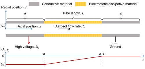
Figure 1. The simplified schematic of a DMA sample outlet, where x is the axial position along the tube, r is the radial position, R is the inner radius of the tube, U₀ is the negative high voltage applied to the high electric potential region, Q is the aerosol flow rate through the tube, a is the length of the high electric potential region, b is the length of the grounded region, and L is the length between the high and low electric potential regions. The relationship between the electric potential on the inner surface of the tube, U(x, R), and the axial position, x, is a boundary condition for solving the electric potential inside the tube. The classified particles are assumed to be positively charged.

The analytically solved electric field was compared to the electric field obtained using the numerical method proposed by Tammet (2015), and there is no significant difference between the two solutions (see SI Figure S1).

The electric field lines within the ESD tube are nearly uniform and parallel (as shown in Figure 2a). The axial electric field intensities at different radial positions in the middle of a long tube (i.e., x = a + L/2) are all equal to U₀/L, and the radial electric field intensities are zero (Figures 2b and c). The parallelism of the electric field near the ends of the ESD tube (i.e., x = a and x = a + L) is distorted, resulting in the high radial electric field intensities. Tammet (2015) reported that the electric field within the tube may not be uniform when L is short. However, uniformity is observed for the simulated electric field, even at the shortest length (L = 0.01 m, i.e., L/R = 5) in this study (Figure 2d). We did not explore the electric field and transmission of particles using a length smaller than 0.01 m because a relatively long tube is preferable for reducing particle losses through an adverse axial electric field. The exact values of a and b may be difficult to determine for a DMA sample outlet. However, U_{(x, r)} is insensitive to a and b when they are larger than 3 R (see SI Figure S2); thus it is reasonable to use U₀, L, and R as the governing parameters for the electric field.

Figure 2. The analytically solved electric fields for the electrical dissipative tube. U₀= −1 V and R = 2 mm. (a) The electric field lines when L = 0.1 m; (b) the axial electric field when L = 0.1 m; (c) the radial electric field when L = 0.1 m; (d) the axial electric field when L = 0.01 m. U₀ is the voltage applied to the high electric potential region. According to Equation (1)(1) $$\begin{array}{l}{U}_{\left(x,r\right)}=U_0\cdot \left(1-\frac{x}{a+L+b}\right)+\\ \times \sum _{i=1}^{+\infty }\left\{\frac{2U_0\left(a+L+b\right)}{i^2{\pi }^{2}L}\left[\text{sin}\hspace{0.17em}\left(\frac{i\pi a}{a+L+b}\right)-\hspace{0.17em}\text{sin}\hspace{0.17em}\left(\frac{i\pi \left(a+L\right)}{a+L+b}\right)\right]\cdot \hspace{0.17em}\text{sin}\hspace{0.17em}\left(\frac{i\pi x}{a+L+b}\right)\cdot I_0\left(\frac{i\pi r}{a+L+b}\right)/I_0\left(\frac{i\pi R}{a+L+b}\right)\right\}\end{array},$$(1) , the electric field intensity is linearly proportional to U₀. L is the length of the electrical dissipative tube. R is the inner radius of the tube. The dashed lines indicate the axial positions of the ends of the electrostatic dissipative tube (corresponding to x = a and x = a + L in Figure 1).

2.2. Simplified analytical model for transmission efficiency

A simplified analytical model for estimating particle transmission efficiency through an adverse axial electric field is proposed. The major approximations of the simplified analytical model are as follows: (a) the air flow profile inside the cylindrical tube follows a uniform distribution or the Hagen-Poiseuille equation; (b) the axial length where particles move as a result of the radial electric field is negligible compared to the total length of the tube; (c) the electric field does not affect the diffusive loss rate. Both particle electrostatic migration and diffusion are considered in the simplified analytical model. In this model, the transmission efficiency of charged particles through an adverse axial electric field with diffusion is calculated as: (3) $$\eta =\frac{2\pi \cdot {\int }_0^{r_{\xi }}n\left(\mu ,r\right)\cdot u\left(r\right)\cdot r\cdot \mathrm{d}r}{n_0\cdot Q}$$(3) (4) $$\mu =\frac{\pi D{L}_{\text{total}}}{Q}$$(4) (5) $$r_{\xi }=\{\begin{array}{l}R\cdot \sqrt{1-\sqrt{\min \left(\xi ,2\right)-\min {\left(\xi ,2\right)}^2/4}}\text{for} \\ \text{Hagen}-\text{Poiseuille} \text{flow}\\ R\cdot \sqrt{\max (1-\xi ,0)}\text{for} \text{plug} \text{flow}\end{array}$$(5) (6) $$\xi =-\frac{Z\cdot E}{u_{\text{ave}}}$$(6) where η is the transmission efficiency; n(μ,r) is the particle number concentration at radial position r and dimensionless length μ, as defined in Equation (4)(4) $$\mu =\frac{\pi D{L}_{\text{total}}}{Q}$$(4) ; L_total is the total diffusion length; n₀ is the initial uniform particle number concentration; u(r) is the air flow velocity at r; r_ξ is the threshold radius defined in Equation (5)(5) $$r_{\xi }=\{\begin{array}{l}R\cdot \sqrt{1-\sqrt{\min \left(\xi ,2\right)-\min {\left(\xi ,2\right)}^2/4}}\text{for} \\ \text{Hagen}-\text{Poiseuille} \text{flow}\\ R\cdot \sqrt{\max (1-\xi ,0)}\text{for} \text{plug} \text{flow}\end{array}$$(5) (see its derivation in the SI); ξ is a dimensionless parameter that characterizes the transmission efficiency through the adverse axial electric field (Attoui and Fernández de la Mora 2016); Z is the electrical mobility of charged particles; E is the axial electric field intensity equal to U₀/L; and u_ave is the mean air flow velocity. Note that μ in Equation (4)(4) $$\mu =\frac{\pi D{L}_{\text{total}}}{Q}$$(4) is actually a nondimensionalized length that corresponds to x = L_total, and, in the notation of the SI, it should be written as μ_total = μ(L_total); however, we keep the symbol μ in the main text for simplicity. Particles with an initial radial position beyond r_ξ are lost to walls because of electrostatic migration upon entering the adverse electric field. Although U₀, E, and Z are defined as signed scalars in this study, Equation (6)(6) $$\xi =-\frac{Z\cdot E}{u_{\text{ave}}}$$(6) ensures that ξ is always non-negative in an adverse electric field. When n(μ,r) and u(r) are fixed, an increasing adverse electric field intensity leads to an increasing ξ and decreasing r_ξ and thereby a decreasing transmission efficiency η.

The values of u(r) and n(μ,r) are affected by the air flow profile. In this study, we consider three idealized flow profiles: Hagen-Poiseuille flow, plug flow, and turbulent flow. The Hagen-Poiseuille flow is a fully developed laminar flow, and u(r) follows a parabolic profile. The plug flow is an undeveloped laminar flow, and u(r) is uniform. The expressions for n(μ,r) for both the Hagen-Poiseuille flow and plug flow are given in SI Equation (S34). In the turbulent flow, the fluid molecules and particles are assumed to be perfectly mixed in the radial direction but not in the axial direction; hence, u(r) and n(μ,r) are both uniform in every cross section of the tube. A schematic of u(r) and n(μ,r) for these three flow profiles is shown in SI Figure S3. The flow profile can be presumed according to the Reynolds number and the entrance length of the tube, as illustrated by Tammet (2015), or determined empirically according to the measured transmission efficiencies at different ξ values (as shown in section 4.2).

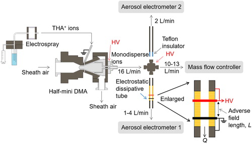
Figure 3. The schematic of the experimental setup for characterizing the transmission efficiencies through the electrostatic dissipative tube. The blue tube is made of Teflon, the yellow tube is made of electrical dissipative material, and the dark gray tube is made of stainless steel. The adverse field length, L, is changed by adjusting the distance between the high voltage ring and the grounded ring. The sample outlet of the half-mini DMA is not grounded, such that the tube upstream of the cross fitting has the same electric potential as the central electrode of the half-mini DMA.

Assuming that the air flow is turbulent, electrostatic and diffusional losses can be considered separately because u(r) is uniform, and the shape of n(μ,r) can be considered approximately independent of μ. Accordingly, the overall transmission efficiency is equal to the product of the transmission efficiency considering diffusional loss and electrostatic loss, as follows: (7) $$\eta ={\eta }_{\text{diff}}\cdot {\eta }_{\text{elec}}={\eta }_{\text{diff}}\cdot \max \left(1-\xi ,0\right)\text{for} \text{turbulent} \text{flow},$$(7) where η_diff is the transmission efficiency for diffusional loss only, and η_elec is the transmission efficiency for electrostatic loss only. The value of η_diff for turbulent flow is given in Brockmann (2011). The expression for η_elec is the same as the formula for non-diffusive particles in a plug flow (SI Equation (S28)) proposed by Tammet (2015) and the reduced form of the above simplified analytical model when μ is zero.

For convenience of discussion, the minimum ξ corresponding to a zero transmission is defined as ξ₀. The air flow profile can be investigated using ξ₀, e.g., the values of ξ₀ are 2.0, 1.0, and 1.0 for Hagen-Poiseuille flow, plug flow, and turbulent flow, respectively. When ξ exceeds ξ₀, theoretically no particle passes through the adverse electric field.

Substituting the centroid electrical mobility predicted using the transfer function of DMA (Knutson and Whitby 1975) into Equation (6)(6) $$\xi =-\frac{Z\cdot E}{u_{\text{ave}}}$$(6) , the ξ value for particles through the adverse axial electric field inside the sample outlet of a DMA can be expressed as: (8) $$\xi =\frac{Q_c+Q_m}{4\Lambda }\cdot \frac{R^2}{L\cdot Q},$$(8) where Q_c and Q_m are the sheath flow rate and excess flow rate of the DMA, respectively; Λ is the geometric factor of the DMA; and Q is the aerosol sample flow rate through the ESD tube.

As shown in Equation (8)(8) $$\xi =\frac{Q_c+Q_m}{4\Lambda }\cdot \frac{R^2}{L\cdot Q},$$(8) , ξ is the same for particles with different diameters at a given DMA flow configuration because E is linearly proportional to U₀, while the classified aerosol electrical mobility Z, is inversely proportional to U₀. At a given DMA configuration, the electrostatic losses can be reduced by increasing the length of the ESD tube, L, and decreasing the inner radius of the tube, R.

2.3. Monte-Carlo simulation

The transmission of charged particles through an adverse axial electric field was also simulated using the Monte-Carlo method. The initial position of each particle was generated randomly. Particle diffusion was simulated using the random walk method. During each time step, dt, the Brownian motion in the axial direction follows a normal distribution with a standard deviation of $\sqrt{2D\cdot \mathrm{d}t},$ where D is the diffusion coefficient of particles. Because of the high Péclet numbers (>2000) in the test conditions, the effect of Brownian motion in the axial direction on the simulation results was found not to be insignificant. Whether to consider the Brownian motion in the axial direction or not does not affect the simulation results significantly because of the high Péclet numbers (>2000) in the test conditions. The Brownian motion in the radial direction is non-symmetric (for further illustrations, please refer to the SI of Mai and Flagan [2018]): (9) $$r\left(t+\mathrm{d}t\right)=\sqrt{{\left[r\left(t\right)+\mathrm{d}r\right]}^2+{\left[r\mathrm{d}\theta \right]}^2}=\sqrt{{\left[G\left(r\left(t\right),\sqrt{2D\cdot \mathrm{d}t}\right)+Z\cdot E_r\cdot \mathrm{d}t\right]}^2+{\left[G\left(0,\sqrt{2D\cdot \mathrm{d}t}\right)\right]}^2},$$(9) where dr and rdθ are the particle displacements in the radial and tangential directions, respectively; $G(r(t),\sqrt{2D\cdot \mathrm{d}t})$ denotes a random variable that follows a normal distribution with an expected value of r(t) and a standard deviation of $\sqrt{2D\cdot \mathrm{d}t};$ Z is the electrical mobility of the simulated particle; and $Z\cdot E_r\cdot \mathrm{d}t$ is the particle displacement due to the radial electric force during dt. Note that r(t)+dr calculated this way may sometimes be negative on account of diffusion, while r(t+dt) was forced to always be non-negative for the convenience of simulation. However, Equation (9)(9) $$r\left(t+\mathrm{d}t\right)=\sqrt{{\left[r\left(t\right)+\mathrm{d}r\right]}^2+{\left[r\mathrm{d}\theta \right]}^2}=\sqrt{{\left[G\left(r\left(t\right),\sqrt{2D\cdot \mathrm{d}t}\right)+Z\cdot E_r\cdot \mathrm{d}t\right]}^2+{\left[G\left(0,\sqrt{2D\cdot \mathrm{d}t}\right)\right]}^2},$$(9) has the potential risk that even for non-diffusive particles, they may go across the tube axis through electrostatic migration.

The codes for simulation were written in Julia to save computation time. A total of 10⁴ particle trajectories were simulated to obtain the transmission efficiency for one test condition. The time step, dt, is 10⁻⁵ s, and it was determined after examining the simulation results at different time steps when using the shortest axial electric field among the test conditions (see SI Figure S4).

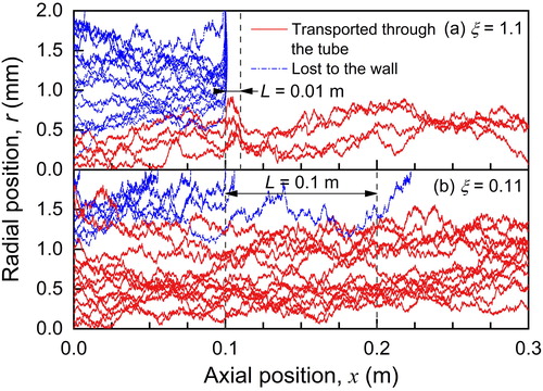
Figure 4. Examples of simulated particle trajectories through (a) a relatively strong and (b) a relatively weak adverse electric field using the Monte-Carlo method. U₀= −300 V, d_p=1.48 nm, Q = 2 L min⁻¹, R = 2 mm, and a = b = 0.1 m (see Figure 1 for their definitions). The air flow is assumed to be Hagen-Poiseuille flow. The dashed lines indicate the approximate end positions of the adverse electric field. For the convenience of illustration, the initial positions of the simulated particles in this figure are assumed to be evenly distributed along the radius rather than determined randomly. The significant particle radial displacement at x = 0.1 m in (a) is mainly caused by the strong radial electric field, and most of the scavenged particles are deposited at x = 0.1 m. In contrast, the radial displacement in (b) is mainly due to random Brownian motion, and particle disposition places are also random.

When assuming that the air flow profile follows the Hagen-Poiseuille equation and there is no adverse electric field, the simulated transmission efficiency agrees well with the analytical solution proposed by Gormley and Kennedy (1949), indicating the validity of the Monte-Carlo simulation (SI Figure S5).

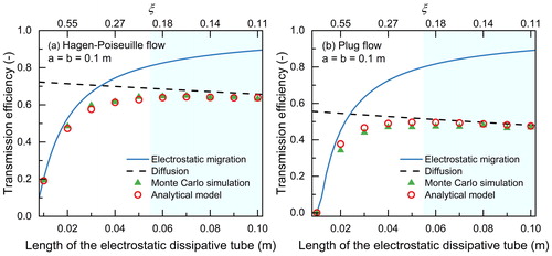
Figure 5. The transmission efficiencies through a DMA sample outlet when assuming the flow is (a) Hagen-Poiseuille flow and (b) plug flow, respectively. U₀= −300 V, d_p = 1.48 nm, R = 2 mm, and Q = 2 L min⁻¹ (see Figure 1 for their definitions). Both electrostatic migration and diffusion are considered in the Monte-Carlo simulation and the simplified analytical model. The adverse field length (L) is assumed to be equal to the ESD tube length (because the transmission efficiency is the highest when the total length of the tube is minimized, while the tunable metal rings in Figure 3 are only used for testing). The solid and dashed lines indicate the transmission efficiencies when considering only the particle electrostatic migration (Tammet 2015, or Equation (3)(3) $$\eta =\frac{2\pi \cdot {\int }_0^{r_{\xi }}n\left(\mu ,r\right)\cdot u\left(r\right)\cdot r\cdot \mathrm{d}r}{n_0\cdot Q}$$(3) with μ = 0 and SI Equation (S34)) and only the particle diffusion (Gormley and Kennedy 1949, or Equation (3)(3) $$\eta =\frac{2\pi \cdot {\int }_0^{r_{\xi }}n\left(\mu ,r\right)\cdot u\left(r\right)\cdot r\cdot \mathrm{d}r}{n_0\cdot Q}$$(3) with μ = 0 and SI Equation (S34)), respectively. The recommended range of the tube length is shadowed with light blue. Note that the values of ξ were calculated using the length of the electrostatic dissipative tube; hence, the ξ-axis is nonlinear.

In a turbulent flow, turbulent diffusion is assumed to be dominant and particle transmission is assumed to be completely decoupled into η_diff and η_elec, as shown in Equation (7)(7) $$\eta ={\eta }_{\text{diff}}\cdot {\eta }_{\text{elec}}={\eta }_{\text{diff}}\cdot \max \left(1-\xi ,0\right)\text{for} \text{turbulent} \text{flow},$$(7) . For non-diffusive particles, η_elec is simulated using the Monte-Carlo method by assigning 0 to D.

3. Experiments

The ESD material used in this study is polyoxymethylene copolymer (POM-C, Ensinger Inc.) with a measured specific volume resistance of 3 × 10⁶ Ω m. Theoretically, the electric field inside a tube is independent of the resistance of the tube as long as the electric potential on the surface of the tube decreases linearly; however, a tube with a resistance that is too small will be significantly heated when high voltages are applied. The raw materials were machined into a rigid tube and conductive silver paste was applied on both ends of the tube to reduce contact resistance. Soft ESD polyurethane tubing (e.g., from Freelin-Wade Inc.) was used in Attoui and Fernández de la Mora (2016) for its convenience in reducing contact resistance; however, we use rigid tubing made from POM-C in this study for its better mechanical strength.

The homogeneity of the ESD material was tested. The measured accumulative voltage drop is linearly proportional to the accumulative tube length when an electric potential difference is applied along the ESD material (SI Figures S6 and S7), indicating that the boundary condition of the electric field is valid, i.e., that the electric potential on the surface of the tube decreases linearly along the tube.

Figure 6. The transmission efficiencies through the sample outlet of a DMA when assuming a = 0.9 m and b = 0.1 m. The air flow is (a) Hagen-Poiseuille flow and (b) turbulent flow. Both electrostatic migration and diffusion are considered in the simplified analytical model. U₀= −300 V, d_p=1.48 nm, R = 2 mm, and Q = 2 L min⁻¹ (see Figure 1 for the definitions). The recommended range of the tube length is shadowed with light blue. Note that the values of ξ were calculated using the length of the electrostatic dissipative tube, and the ξ-axis is nonlinear.

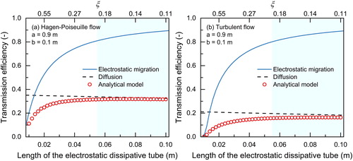
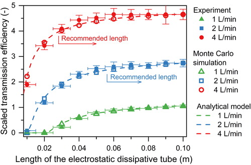
Figure 7. The scaled transmission efficiencies of 1.48-nm ions through the electrostatic dissipative tube from experiments, the simplified analytical model, and the Monte-Carlo simulation. The experimentally determined scaled transmission efficiency is the measured number concentration ratio of aerosol electrometer 1 to aerosol electrometer 2 (see Figure 3). Particle diffusion was considered separately when using the Monte-Carlo method for the turbulent flow (as illustrated in section 3.1). The vertical error bar indicates three times the standard deviation of the measured data. The adverse field length, L, was manually adjusted, and the uncertainties were estimated to be less than 0.005 m. Accordingly, 0.005 m was used as the half-length of the horizontal error bar in the figure.

The transmission efficiencies of ions through the ESD tube with different adverse field lengths were experimentally studied (Figure 3). Monodisperse tetra-heptyl ammonium ions (THA⁺) with an electrical mobility diameter of 1.48 nm were generated using electrospray and subsequently classified using a half-mini DMA (Fernández de la Mora and Kozlowski 2013; Ude and Fernández de la Mora 2005). The diameter, 1.48 nm, is estimated using the inverse electrical mobility reported in Ude and Fernández de la Mora (2005). Please note that it is slightly different than the reported diameters, i.e., 1.47 nm in Ude and Fernández de la Mora (2005) and 1.45 nm in Stolzenburg et al. (2018), because of the differently assumed parameters (see the SI for details). The voltage on the DMA inner electrode was −300 V, and the external electrode was grounded. The sample outlet of the half-mini DMA was modified such that the voltages of the outlet tube and the downstream cross fitting (see Figure 3) were also −300 V. The classified ions were measured by two aerosol electrometers. The linearity of particle number concentrations recorded by these two electrometers was compared before and after each experiment. For the electrometers, zero drifts were minimized and corrected. The ESD tube was deployed before aerosol electrometer 1. Two tight metal rings on the ESD tube were used to adjust the tube length between the high electric potential region and the grounded region. Because the two metal rings are connected to the high electric potential and ground, the surface electric potential changes linearly along the tube between the two metal rings, rather than along the entire ESD tube. As a result, the length between the two adjustable metal rings is the adverse field length, L. Note that the two metal rings are used for adjusting L in this experiment; however, they are not necessarily used in a DMA sample outlet made of ESD tubing.

The voltages upstream and downstream of the two rings are −300 V and 0 V, respectively. Aerosol electrometer 2 was used as a reference and was insulated from the sample outlet with a Teflon connector used as the voltage insulator.

To ensure the relative comparability of the ratios measured at different flow rates, the aerosol flow rate through the Teflon connector was kept constant at 2 L min⁻¹ while the aerosol flow rate through the ESD tube was varied from 1 to 4 L min⁻¹, and the aerosol outlet flow rate of the half-mini DMA was kept constant at 16 L min⁻¹ by adjusting the mass flow controller. Given the latter, the flow upstream of the ESD tube is turbulent. The flow inside the ESD tube may also be turbulent because the length required for a fully developed laminar flow was estimated to be ∼0.28 m at a flow rate of 4 L min⁻¹ and the tested ESD tube length is ∼0.12 m.

Because the classified particles have to be transported against an adverse electric field before being measured by a grounded aerosol electrometer and particle electrostatic losses inside the Teflon connector are unknown, we could obtain only the ratio of the particle number concentrations measured by the two aerosol electrometers rather than the transmission efficiency. The measured particle number concentration and the theoretically predicted transmission efficiencies using the simplified analytical model and Monte-Carlo simulation were scaled for their comparison. The particle number concentration downstream of the ESD tube measured by aerosol electrometer 1 was scaled by dividing it by the number concentration measured by reference aerosol electrometer 2. The physical lengths upstream of the two electrometers are equal; hence, the scaled particle number concentration is mainly determined by the electrostatic losses in both the ESD tube and the Teflon connector. For the convenience of comparison, the theoretical transmission efficiencies were scaled by multiplying by a flow-rate-dependent factor such that the scaled efficiencies at the maximum test length (L = 0.1 m) are the same as their corresponding scaled particle number concentration (i.e., ratios of the two electrometers).

4. Results and discussion

4.1. Ideal tube length for optimized transmission

The transmission efficiency through the adverse electric field is limited by both electrostatic and diffusional losses. According to Equation (8)(8) $$\xi =\frac{Q_c+Q_m}{4\Lambda }\cdot \frac{R^2}{L\cdot Q},$$(8) for ξ, particle electrostatic loss is positively related to the inner radius of the tube (R) and negatively related to the ESD tube length (L) and aerosol flow rate (Q). According to Equation (4)(4) $$\mu =\frac{\pi D{L}_{\text{total}}}{Q}$$(4) for μ, particle diffusional loss is positively related to L and negatively related to Q. Accordingly, the transmission efficiency of charged particles through a DMA sample outlet increases monotonically with increasing Q and decreasing R. However, the value of Q is usually determined by the DMA configuration, and R is usually determined by the geometrical design of the DMA and the downstream tube. Extending L is perhaps the most practical way to reduce electrostatic losses without changing the configuration of a DMA. A larger L corresponds to a smaller ξ, which corresponds to a decreased particle electrostatic loss. However, particle diffusional loss increases with the length of a sample outlet tube. As in the examples shown in Figure 4, electrostatic migration is the major cause of particle losses when the electric field is relatively strong (ξ = 1.1), while diffusion contributes more to particle losses than electrostatic migration does when the electric field is relatively weak (ξ = 0.11).

Although particle transmission is determined by both μ and ξ, Figure 5 shows that under the test conditions given there, the ideal length of the ESD tube for the sample outlet of the half-mini DMA is determined mainly by ξ. The overall transmission efficiency is some value smaller than both the efficiency considering diffusional loss alone and that considering electrostatic loss alone. Under these test conditions, the transmission efficiency stabilizes when ξ is smaller than 0.2. Extending L when ξ is smaller than 0.2 does not decrease the overall loss of particles effectively because ξ is inversely proportional to L while diffusional loss is positively related to L. Using the simplified analytical model or Monte-Carlo simulation, it is possible to estimate the optimal tube length corresponding to the maximum transmission efficiency under the test conditions.

In practical applications, the aerosol concentration profile, n(r), and air flow profile, u(r), are sometimes difficult to determine exactly (Stolzenburg 2018). As a result, particle diffusional losses inside a DMA, especially for sub-3-nm particles, are still not well understood. In addition, diffusional loss varies with the classified particle diameter in the same electric field and air flow field. Accordingly, it is more reasonable to determine a range of ideal tube length corresponding to relatively high transmission efficiencies than to determine a single optimal tube length. Without loss of generality, we assume that the effective diffusion length of the sample outlet is a large value, 1.0 m, to further explore the ideal length of the ESD tube when the diffusional loss inside the entire tube is relatively high. The diffusion length is treated as a length of an actual tube. As shown in Figure 6, the transmission efficiency through a 1.0-m tube is also relatively constant when ξ is smaller than 0.2 for both Hagen-Poiseuille flow and turbulent flow. Thus, it is found that for the half-mini DMA a criterion value of 0.2 for ξ is valid for determining the ideal tube length under the various test conditions in this study. This criterion is mainly for small particles (e.g., <3 nm). When classifying only large particles (e.g., >20 nm), whose diffusional losses become less important, particle transmission efficiency increases monotonically with decreasing ξ; hence, the criterion value can be further decreased to improve the transmission efficiency.

According to the theoretical analysis above, the optimal ESD tube length for the half-mini DMA, L, can be inferred from the ξ criterion value using Equations (6)(6) $$\xi =-\frac{Z\cdot E}{u_{\text{ave}}}$$(6) or (8) in practical applications. To ensure relatively high transmission efficiencies at various DMA flow configurations, L should be determined for the most unfavorable condition, i.e., the lowest sample flow rate (Q) and the highest sheath and excess flow rates (Q_c and Q_m), hence, the highest voltage (U₀). As shown in Figures 5 and 6, L can be determined as some value larger than –5Z·U₀/u_ave (and perhaps smaller than ∼–20Z·U₀/u_ave to avoid potentially large diffusional loss and long residence time).

Please note that the criterion above is valid for these test conditions of the half-mini DMA, whereas its feasibility for other conditions remains to be explored. Theoretically, when the Q is lower and/or R is larger, i.e., the adverse electric field intensity is relatively stronger, L needs to be extended to reduce particle electrostatic losses while particle diffusional loss is correspondingly larger. As a result, the optimal ξ value for the maximum transmission efficiency may be larger than 0.2 under other conditions beyond the test.

4.2. Experimentally measured transmission

As shown in Figure 7, the normalized measured ratio agrees with the transmission efficiency predicted using the simplified analytical model for turbulent flow (Equation (7)(7) $$\eta ={\eta }_{\text{diff}}\cdot {\eta }_{\text{elec}}={\eta }_{\text{diff}}\cdot \max \left(1-\xi ,0\right)\text{for} \text{turbulent} \text{flow},$$(7) ) and the Monte-Carlo simulation for particles neglecting Brownian diffusion. The turbulent flow was derived according to ξ₀ and the fitted diffusion length. The air flow profile inside the tested tube is uniform because the experimentally determined ξ₀ is ∼1.0 (nearly no particles were measured downstream of the ESD tube when ξ was larger than 1.0), indicating that the flow corresponds to plug flow or turbulent flow. The scaled transmission efficiency from the simplified analytical model was compared to the measured ratios of the two electrometers at various assumed particle number concentration profiles, and the best fit occurred when the particle number concentration profile was nearly uniform at every cross section of the tube (turbulent flow). The turbulence in the upstream aerosol outlet of the half-mini DMA is perhaps the cause of the turbulence in the tested ESD tube (as discussed in section 3.2). Similarly to this study, Attoui and Fernández de la Mora (2016) reported that the analytical formula proposed by Tammet (2015) for non-diffusive particles in a plug flow (the same as the formula for η_elec in Equation (7)(7) $$\eta ={\eta }_{\text{diff}}\cdot {\eta }_{\text{elec}}={\eta }_{\text{diff}}\cdot \max \left(1-\xi ,0\right)\text{for} \text{turbulent} \text{flow},$$(7) ) achieved a good fit for highly diffusive sub-3-nm ions, which is probably because the air flow was actually turbulent. It should be clarified that although in good accordance with the Monte-Carlo simulation under these test conditions, the simplified analytical model may be inaccurate when its major approximations are strongly violated.

According to the simplified analytical model, a ξ smaller than the recommended criterion of 0.2 corresponds to a transmission efficiency larger than 80% of the maximum efficiency for any of the three air flow profiles. As shown in Figure 7, when the aerosol flow rate through the ESD tube is 2 L min⁻¹, the transmission efficiency at the minimum recommended length of –5Z·U₀/u_ave (0.056 m) is 90% of the measured maximum transmission efficiency at a length of 0.1 m and the same aerosol flow rate. Accordingly, when aiming to improve particle transmission through the half-mini DMA outlet, it is not critical to distinguish the exact flow profile.

4.3. Application example

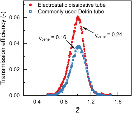
Based on the above findings, the ESD tube (POM-C, Ensinger Inc.) was used to increase the transmission efficiency through the sample outlet of a mini-cy DMA (Cai et al. 2017). The insulation Delrin used between the central electrode and the original metal outlet tube was replaced with a rigid ESD tube. The length of the original Delrin tube was 0.006 m, which was determined in a previous study to correspond to the highest penetration efficiency among the tested dimensions. Due to the similarity in the geometry of the mini-cy DMA outlet and the half-mini DMA outlet, the ESD tube length is determined according to section 4.1. Under the most unfavorable condition for ξ (a sheath flow rate of 30 L min⁻¹ and an aerosol flow rate of 1 L min⁻¹), the tube length corresponding to −10Z·U₀/u_ave is 0.04 m, and the practical length of 0.05 m was used to leave some space for tubing connection. The total length of the new sample outlet made of ESD tube is 0.02 m longer than the total length of the original sample outlet. Tetra-heptyl ammonium (THA⁺) ions with an electrical mobility diameter of 1.48 nm were used to characterize the penetration efficiencies of the DMA. The experimental setup is similar to that reported in Cai et al. (2017). The transfer functions of 1.48-nm ions for the DMA using the original and new sample outlets were measured. The penetration efficiency was fitted using the diffusive transfer function (Stolzenburg 2018).

The penetration efficiency through the mini-cy DMA was improved using the new sample outlet made of the ESD tube. At a sheath flow rate of 25 L min⁻¹, the penetration efficiencies of 1.48-nm ions using the original and new sample outlets were 16% and 24%, respectively, at an aerosol flow rate of 1.5 L min⁻¹ (Figure 8); they were 20% and 26%, respectively, at an aerosol flow rate of 2.5 L min⁻¹. The improvement is higher at a lower aerosol flow rate because the electrostatic loss in the original sample outlet is significant, while it contributes to only a minor proportion of particle loss in the new sample outlet.

Figure 8. The measured transfer functions of 1.48-nm ions for a miniature cylindrical DMA using the original sample outlet made of Delrin and the new outlet made of a rigid electrical dissipative tube. The electrical mobility is $\tilde{Z},$ normalized by the measured centroid electrical mobility, and η_pene is the fitted DMA penetration efficiency characterizing particle losses inside the DMA, i.e., the area between the fitted transmission efficiency curve and the horizontal axis.

5. Summary

We explored the transmission efficiency of charged particles and ions through an adverse axial electric field, e.g., a DMA sample outlet. The electric field inside a DMA sample outlet made of ESD tubing was solved analytically. The transmission of charged particles through the adverse electric field was evaluated using both a simplified analytical model and the random walk Monte-Carlo method. The transmission efficiency through the ESD tube was also experimentally measured. The homogeneity of the ESD tubing used in this study was verified. The measured transmission efficiencies agree with both the simplified analytical model and the Monte-Carlo simulation. However, the validity of the simplified analytical model under other conditions beyond the tests in this study still needs to be tested further. Although the flow field and particle diffusion in a real DMA sample outlet are usually complex, the length of the ESD tube corresponding to relatively high transmission efficiency of the DMA under the test conditions can be practically determined using a rough criterion: the tube length is longer than the threshold value that corresponds to a ratio of particle electrostatic migration velocity to average air flow velocity (ξ) smaller than 0.2. Based on these theoretical analyses, the commonly used Delrin insulator at the sample outlet of a miniature cylindrical DMA was replaced by an ESD tube to reduce electrostatic loss. Accordingly, the penetration efficiency of 1.48-nm ions under typical operating conditions (a sheath flow rate of 25 L min⁻¹ and an aerosol flow rate of 1.5 L min⁻¹) was increased by 50%, because using the ESD tube decreased the adverse electrostatic field.

Acknowledgments

The authors thank Michel Attoui at UPEC for helpful discussions, Hannes Tammet at University of Tartu for sharing his codes for numerically solving the electric field and simulating particle trajectories, and the two anonymous reviewers for their valuable comments and their careful checking of the equations.

Additional information

Funding

Financial supports from National Key R&D Program of China (2017YFC0209503), the National Natural Science Foundation of China (21876094), and State Key Joint Laboratory of Environment Simulation and Pollution Control (17K10ESPCT) are acknowledged.

References

- Attoui, M., and J. Fernández de la Mora. 2016. Flow driven transmission of charged particles against an axial field in antistatic tubes at the sample outlet of a differential mobility analyzer. J. Aerosol Sci. 100:91–96. doi:10.1016/j.jaerosci.2016.06.002.
- Bezantakos, S., L. Huang, K. Barmpounis, M. Attoui, A. Schmidt-Ott, and G. Biskos. 2015. A cost-effective electrostatic precipitator for aerosol nanoparticle segregation. Aerosol Sci. Technol. 49 (1):iv–vi. doi:10.1080/02786826.2014.1002829.
- Brockmann, J. E. 2011. Aerosol transport in sampling lines and inlets. In Aerosol measurement: Principles, techniques, and applications, eds. P. Kulkarni, P. A. Baron, and K. Willeke, 3rd ed., 90–91. Hoboken, NJ: Willey & Sons, Inc.
- Cai, R., D.-R. Chen, J. Hao, and J. Jiang. 2017. A miniature cylindrical differential mobility analyzer for sub-3 nm particle sizing. J. Aerosol Sci. 106:111–119. doi:10.1016/j.jaerosci.2017.01.004.
- Cai, R., J. Jiang, S. Mirme, and J. Kangasluoma. 2019. Parameters governing the performance of electrical mobility spectrometers for measuring Sub-3 nm particles. J. Aerosol Sci. 127:102–115. doi:10.1016/j.jaerosci.2018.11.002.
- Chen, D.-R., and D. Y. H. Pui. 1999. A high efficiency, high throughput unipolar aerosol charger for nanoparticles. J. Nanoparticle Res. 1 (1):115–126. doi:10.1023/a:1010087311616.
- Chen, D.-R., D. Y. H. Pui, D. Hummes, H. Fissan, F. R. Quant, and G. J. Sem. 1998. Design and evaluation of a nanometer aerosol differential mobility analyzer (nano-DMA). J. Aerosol Sci. 29 (5–6):497–509. doi:10.1016/S0021-8502(97)10018-0.
- Fernández de la Mora, J., and J. Kozlowski. 2013. Hand-held differential mobility analyzers of high resolution for 1–30 nm particles: Design and fabrication considerations. J. Aerosol Sci. 57:45–53. doi:10.1016/j.jaerosci.2012.10.009.
- Flagan, R. C. 2011. Electrical mobility methods for submicrometer particle characterization. In Aerosol measurement: Principles, techniques, and applications, eds. P. Kulkarni, P. A. Baron, and K. Willeke, 339–363. New York: John Wiley & Sons.
- Franchin, A., A. Downard, J. Kangasluoma, T. Nieminen, K. Lehtipalo, G. Steiner, H. E. Manninen, T. Petäjä, R. C. Flagan, and M. Kulmala. 2016. A new high-transmission inlet for the caltech nano-RDMA for size distribution measurements of Sub-3 nm ions at ambient concentrations. Atmos. Measur. Tech. 9 (6):2709–2720. doi:10.5194/amt-9-2709-2016.
- Gormley, P. G., and M. Kennedy. 1949. Diffusion from a stream flowing through a cylindrical tube. Proc. R. Irish Acad. A 52:163–168.
- Iida, K. 2008. Atmospheric nucleation: Development and application of nanoparticle measurements to assess the roles of ion-induced and neutral processes. Minneapolis: University of Minnesota.
- Knutson, E. O., and K. T. Whitby. 1975. Aerosol classification by electric mobility: Apparatus, theory, and applications. Aerosol Sci. Technol. 6 (6):443–451. doi:10.1016/0021-8502(75)90060-9.
- Kousaka, Y., K. Okuyama, M. Adachi, and T. Mimura. 1986. Effect of Brownian diffusion on electrical classification of ultrafine aerosol particles in differential mobility analyzer. J. Chem. Eng. Jpn. 19 (5):401–407. doi:10.1252/jcej.19.401.
- Mai, H., and R. C. Flagan. 2018. Scanning DMA analysis: I. Classification transfer function [Published Online]. Aerosol Sci. Technol. 52 (12):1382–1399. doi:10.1080/02786826.2018.1528005.
- Stolzenburg, M. R. 2018. A review of transfer theory and characterization of measured performance for differential mobility analyzers. Aerosol Sci. Technol. 52 (10):1194. doi:10.1080/02786826.2018.1514101.
- Stolzenburg, M. R., J. H. T. Scheckman, M. Attoui, H.-S. Han, and P. H. McMurry. 2018. Characterization of the TSI model 3086 differential mobility analyzer for classifying aerosols down to 1 nm. Aerosol Sci. Technol. 52 (7):748–756. doi:10.1080/02786826.2018.1456649.
- Surawski, N. C., S. Bezantakos, K. Barmpounis, M. C. Dallaston, A. Schmidt-Ott, and G. Biskos. 2017. A tunable high-pass filter for simple and inexpensive size-segregation of sub-10-nm nanoparticles. Sci. Rep. 7 (1):45678. doi:10.1038/srep45678.
- Tammet, H. 2015. Passage of charged particles through segmented axial-field tubes. Aerosol Sci. Technol. 49 (4):220–228. doi:10.1080/02786826.2015.1018986.
- Ude, S., and J. Fernández de la Mora. 2005. Molecular monodisperse mobility and mass standards from electrosprays of tetra-alkyl ammonium halides. J. Aerosol Sci. 36 (10):1224–1237. doi:10.1016/j.jaerosci.2005.02.009.