Models for estimating nanoparticle transmission efficiency through an adverse axial electric field

Abstract

An adverse electric field is often encountered or utilized when classifying charged nanoparticles or ions according to their electrical mobility. For instance, the classified charged particles usually have to be transported through an adverse electric field against the aerosol sample flow before exiting the outlet of a differential mobility analyzer (DMA). Recently, we reported the transmission of charged nanoparticles through the DMA adverse axial electric field and its improvements. Herein, the simplified analytical model used in that study and a new simplified numerical model to evaluate particle transmission efficiency through the adverse axial electric field are introduced in detail. In addition to the DMA sample outlet, these models are also tested for the electrical mobility filter (EMF) for segregating charged nanoparticles, especially under the unfavorable conditions when the assumptions for these models are violated. The modeled results are compared to a Monte Carlo method based on single-particle tracking and the experimentally determined transmission efficiencies. For the typical geometries and test conditions of a half-mini DMA sample outlet and the EMF, the mean absolute differences between these models and the Monte Carlo method are less than 1%. However, the accuracy of these models is guaranteed only when their assumptions are satisfied, i.e., when the adverse electric field is longer than 4 times the tube radius so that the field lines are axially parallel and the tube length before the adverse electric field is at least half of the entrance length for the air flow. In addition, the simplified analytical model may deviate from the true transmission efficiency when the adverse electric field is longer than 10% of the entire tube. In such cases that the assumptions for both the simplified analytical model and the simplified numerical model are violated, the Monte Carlo method can be used instead.

Copyright © 2019 American Association for Aerosol Research

1. Introduction

In aerosol studies, it is often encountered that charged nanoparticles or ions are transported against an adverse electric field. For instance, when classifying them according to their electrical mobility using a differential mobility analyzer (DMA, Knutson and Whitby 1975), charged particles and ions migrate along with the electric field in the classification region and then against the adverse electric field in the sample outlet (or inlet in some cases). Their electrostatic losses can be reduced using a specially designed sample outlet or inlet inside which the adverse electric field is axially parallel (Attoui and Fernández de la Mora 2016; Franchin et al. 2016). Based on the same principle, Bezantakos et al. (2015) developed a tunable electrical mobility filter (EMF) that can segregate charged particles using an adjustable adverse axial electric field.

Theoretical analysis of nanoparticle penetration through the adverse axial electric field considering both particle diffusion and electrostatic migration is needed, especially for sub-10-nm particles. Previously, several models were used for characterizing the transmission efficiency of charged particles through an axial electric field. Bezantakos et al. (2015) used a semi-empirical formula considering both electrostatic and diffusional losses. In this formula, four parameters were used to fit experimentally measured transmission efficiency. Different values were obtained for these parameters when instrumental working conditions are different (Bezantakos et al. 2015; Surawski et al. 2017), which limits the application of this semi-empirical formula.

Based on sound theoretical derivation, Tammet (2015) proposed an analytical solution for the transmission efficiency of non-diffusive particles which is a function of one dimensionless parameter. This analytical solution agrees well with experimentally measured transmission efficiency through an EMF when assuming a Hagen-Poiseuille flow (Tammet 2015) and that through the sample outlet of a DMA when assuming a plug flow (Attoui and Fernández de la Mora 2016). Surawski et al. (2017) compared this analytical solution to the transmission efficiency of sub-6 nm particles through an EMF and reported relatively good agreement although particle diffusion is not considered in the solution. However, the electric potential was multiplied by a correction factor of 0.58 and the air flow inside the EMF was assumed to be a plug flow, which is different from the Hagen-Poiseuille flow assumption in Tammet (2015).

In our recent study (Cai, Zhou, and Jiang 2019), a simplified analytical model considering both particle diffusion and electrostatic migration is proposed. This simplified analytical model is a function of only two dimensionless parameters, one for diffusional loss and the other for electrostatic loss. This model was found to be consistent with measured data and the Monte Carlo simulation results in the test conditions for a half-mini DMA. However, the flow and electric fields may vary a lot in real applications. In this simplified analytical model, electrostatic and diffusion losses are considered separately and subsequently coupled together, i.e., particle diffusion loss inside the adverse electric field is simply approximated to be unaffected by the electric field. This rough approximation may limit the validity of this model for other conditions, and thus requires further evaluations.

In this study, we test several methods for estimating the transmission efficiency of charged nanoparticles through the adverse electric field. In addition to the simplified analytical model, a simplified numerical model is proposed and tested. The simplified numerical model estimates particle transmission before, within, and after the adverse electric field separately for better accounting for the influence on the electrostatic field on particle diffusion loss compared to the simplified analytical model. A Monte Carlo method based on single trajectory particle tracking (Cai, Zhou, and Jiang 2019) is used as the benchmark. Note that the names of these models indicate the method to estimate the transmission efficiency while the flow and electric fields are analytically solved for each model. Estimated transmission efficiencies using the Monte Carlo method, the simplified numerical model and the simplified model are compared to the measured efficiencies of an EMF. The performance of two models when their assumptions are violated, which may sometimes be encountered in real applications, is examined.

2. Methods

2.1. Electric fields

A DMA sample outlet and an EMF were used as examples to illustrate the proposed models and their applications. A fraction of charged particles deposits onto the wall of the tube due to the adverse electric field. The tube is axisymmetric in geometry. The variables governing the electric field and particle transmission efficiency for the DMA sample outlet are detailed in Cai, Zhou, and Jiang (2019) and are illustrated in Figure 1. The charged particles enter the tube from a high electric potential region of the sample outlet of a DMA (Figure 1a), while a high voltage is applied to the middle region along the axial direction of the EMF (Figure 1b). U_(x,r) is the electric potential and U₀ is the high potential applied to the DMA central electrode or the EMF; x and r are the axial and radial positions, respectively; L is the length of the adverse electric field; L_total is the total length of the entire tube; R is the tube radius; a and b are the lengths before and after the electrical field, respectively; Q is the aerosol flow rate; d_p is particle diameter; L₂ and L₃ are illustrated in Figure 1b. Particles to be transported through the electric field are assumed to be positively charged, and the corresponding high voltages for the DMA and the EMF are negative and positive, respectively. Note that the following findings will be the same if assuming negatively charged particles, classified using a positive DMA voltage or a negative EMF voltage. Among these variables, U_(x,r), U₀, and particle charge polarity are defined as signed scalars while others are unsigned scalars.

Figure 1. Schematics and the corresponding voltage boundary conditions of (a) a DMA sample outlet made of an electrostatic dissipative tube (reprinted with permission from Cai, Zhou, and Jiang (2019); Copyright 2019 American Association for Aerosol Research) and (b) an electrical mobility filter. Particles are assumed to be positively charged. U_(x,R) is the electric potential on the inner surface of the tube. The electrostatic dissipative materials are used to keep the linearity of changing electric potentials on the surface of the tube. x is the axial position along the tube, r is the radial position, R is the inner radius of the tube, L is the length of the adverse electric field where the voltage on the surface of the tube increases linearly along the axial direction, L_total is the total tube length, Q is the aerosol flow rate through the tube, and U₀ is the applied high voltage.

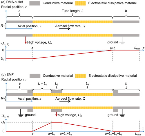
The linearly changing electric potential on the surface of the tube was achieved using electrostatic dissipative (ESD) materials. According to both analytical and numerical solutions for the electric field (Cai, Zhou, and Jiang 2019; Tammet 2015), given a sufficient ratio of L/R, the electric field lines in the middle of the adverse electric field (i.e., x = a + L/2 as illustrated in Figure 1) are uniform and parallel, i.e., the axial electric field intensity, E_x(xmid,r), at x_mid = a + L/2 but different r inside the tube is equal to U₀/L and the radial electric field intensity, E_r(x,r), is zero. Particle electrostatic losses occur only at the entrance of the adverse electric field where the parallelism of the electric field lines is distorted.

For the following models, the electric field is solved analytically under the given conditions of each model. Note that the analytical solution of the electric field (Cai et al. 2019) agrees with the numerical solution (Tammet 2015).

2.2. Simplified numerical model

A simplified numerical model is proposed to estimate particle transmission efficiency through the adverse electric field. This model is derived based on the two assumptions/approximations as follows:

1. The air flow profile remains the same along the axial direction of the cylindrical tube

2. The axial length where particles move as a result of the radial electric field is negligible compared to the length of the adverse electric field

These two assumptions are illustrated by the particle trajectories shown in Figure 2. For the ease of simulation, the air flow is assumed to be a fully developed flow and the flow velocity is independent of the axial position. In this study, we consider only two ideal flow profiles: the Hagen-Poiseuille flow (fully developed laminar flow) and the plug flow. Excluding the effect of the electric field and particle diffusion, particle trajectories inside these flow fields should be axially parallel because there is no radial velocity. However, air flow usually needs a certain length to become fully developed. This length is referred as the entrance length and the flow inside the entrance region is referred as the entrance flow. Within the entrance length of an entrance flow, the flow profile changes gradually along the axial direction and particles move towards the axis of the tube due to the radial flow velocity (Figure 2a). However, the effect of entrance flow on both the electrostatic and diffusion losses are simply neglected in assumption 1) (Figure 2b).

Figure 2. The trajectories of non-diffusive particles through the adverse electric field. The solid and dashed lines are the trajectories of particle transported through the tube and depositing onto the wall, respectively. a = L = b = 0.1 m, R = 2 mm, Q = 2 L/min. (a) The simulated particle trajectories obtained using the single-particle tracking method in an entrance flow, which is implemented in the Monte Carlo method. The dash-dotted lines indicate the approximate entrance and exit positions of the adverse electric field. (b) The assumed particle trajectories in the simplified numerical model and the simplified analytical model. The flow field is assumed to be fully developed and particle electrical displacement in the radial direction is assumed to occur in a negligible axial length. The number-labeled markers indicate the positions of estimated particle concentration profiles (see Figure 3) in the simplified numerical model. The short-dashed line indicates that the radial displacement of a particle at the entrance and exit of the electric field are approximately equal in value due to the symmetric electric field. Note that the trajectories in (b) are not actually used in the simplified numerical model or the simplified analytical model because they directly solve particle concentration profiles.

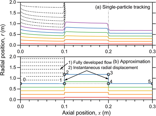
Due to the radial and adverse axial electric fields, the electrostatic losses mainly occur at the entrance of the electric field. Interestingly, in the Hagen-Poiseuille flow where the air flow velocity decreases with the increasing radial position while the adverse electric migration velocity is constant along the radial direction, some particles move backward before they finally deposit on the tube wall (Figure 2a). However, particle displacements due to the radial electric field are simply taken as an instantaneous effect in assumption 2) and, hence, the effect of only the axial electric field is considered when simulating particle diffusion loss in the simplified numerical model. This assumption is acceptable for a relative long adverse electric field (Figure 2) and its validity for a short electric field is discussed below.

In the simplified numerical model, particle diffusion and electrostatic losses are simulated step by step. For the DMA sample outlet, the transmission efficiency is simulated in 5 steps. Diffusion losses are simulated before, within, and after the adverse electric field; and electrostatic migration of particles are simulated at the entrance and exit of the electric field. As shown in Figure 3, the particle cross-sectional concentration profile is uniform at the entrance of the entire tube (position 0). Before the adverse electric field, only particle diffusion is considered and the concentration profile at the entrance of the electric field (position 1) is solved. Due to the radial electric field, particles then migrate towards the tube wall, leading to an expansion of the concentration profile (position 2). According to Gauss’s law, the integral of particle flux of a given particle population is not affected by the electric field unless these particles are scavenged due to their deposition onto the wall (Tammet 1970). The radial position of particles after the electrical migration can be obtained by analytically solving Equation (1)(1) $${\int }_0^{r_1}u\left(r\right)·r·\mathrm{d}r=\mathrm{ }{\int }_0^{r_2}\left[u\left(r\right)+Z·E_x\right]·r·\mathrm{d}r\mathrm{ }\left(r_1\le \mathrm{ }{r}_{\xi }\text{ for the adverse electric field}\right)$$(1) , (1) $${\int }_0^{r_1}u\left(r\right)·r·\mathrm{d}r=\mathrm{ }{\int }_0^{r_2}\left[u\left(r\right)+Z·E_x\right]·r·\mathrm{d}r\mathrm{ }\left(r_1\le \mathrm{ }{r}_{\xi }\text{ for the adverse electric field}\right)$$(1) where r₁ and r₂ are the radial positions before and after the electrical migration, respectively; r_ξ is threshold radius outside of which non-diffusive particles are all scavenged due to the adverse electric field (Cai, Zhou, and Jiang 2019, Equation (5)); u(r) is the air flow velocity as a function of the radial position; Z is the particle electrical mobility, E_x is the axial electric field intensity which is equal to U₀/L, Z·E_x is the electrical migration velocity, and the radial electric field intensity (E_r) is zero because the electric field is uniform and axially parallel. Note that both Z and E_x are defined as signed scalars, hence, Z·E_x is negative for an adverse electric field.

Figure 3. The cross-sectional number concentration profiles of the charged particles inside the tube estimated using the simplified numerical model. The position numbers correspond to the positions of particle trajectories in Figure 2. R is the inner radius of the tube, r is the radial position, n is particle concentration as a function of r, n₀ is particle concentration at the entrance of the tube, and r_ξ is the threshold radius outside of which particles will be scavenged due to the radial electric field. For positions 2 and 3, only the concentration profile of particles migrates along the axial direction is shown. Note that the electrical migration of particles from position 3 to position 4 does not lead to particle loss.

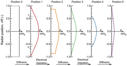
After electrical migration at the entrance of the adverse electric field (position 2), the influence of diffusion on particle concentration profile within the electric field at the exit of the electric field (position 3) is solved numerically. The static electric field does not affect the particle concentration along its trajectory (Tammet 2015). The adverse electric field decreases the net particle velocity (u(r) + Z·E_x) and hence increases its residence time inside the same tube length (L). The increased residence time is partially compensated by the increased radial distance between two adjacent particle trajectories due to the expansion of the particle concentration profile. However, the diffusive loss rate with respect to the axial length, i.e., the diffusive flux towards R, is actually increased in the adverse electric field due to the expansion of particle concentration profile in the radial direction.

The electrical migration of particles at the exit of the adverse electric field (positions 3 to 4) and the diffusional loss after the electric field (positions 4 to 5) are simulated similarly to the method as aforementioned. Finally, particle transmission efficiency through the tube is obtained by calculating integral of concentration flux at the exit of the tube (position 5) and divide it by that at the entrance of the tube (position 0). For the EMF, the transmission efficiency is simulated by 9 steps because the electric field is more complicated than that of the DMA sample outlet.

2.3. Simplified analytical model

To save the computational expense, an additional assumption is added when the electric field is short compared to the total tube length:

1. the electric field does not affect the diffusive loss rate

According to the discussion above, the adverse electric field actually enhances the diffusive loss rate. Hence, this assumption is reasonable only when the diffusion loss inside the electric field is negligible compared to the overall particle losses, which requires a short electric field length (L) compared to the total length of the entire tube (L_total).

Based on assumptions 1) – 3), the electrostatic loss and diffusion of particles can be considered in two separate steps: the first step considering only particle diffusion and the second step considering only the electrostatic loss. In the first step, the particle concentration profile as a result of diffusion is calculated at the exit of the entire tube (Gormley and Kennedy 1949). In the second step, the effect of the electric field is simplified as only removing particles outside the threshold radius, r_ξ, and without changing the trajectories of particles inside it. Similar to the principle for estimating the transmission efficiency when sampling aerosols, ions, and trace gases from the core of a tube to reduce diffusional losses (Fu et al. 2019), the transmission efficiency is then obtained by calculating the integral of particle flux over the area within r_ξ at the exit of the tube and then divide it by the integral at the entrance of the tube. When neglecting the effect of particle diffusion, whether a particle can be transported through the adverse electric field or not is determined by its initial radial position. The value of r_ξ is equal to the derived value of r₁ in Equation (1)(1) $${\int }_0^{r_1}u\left(r\right)·r·\mathrm{d}r=\mathrm{ }{\int }_0^{r_2}\left[u\left(r\right)+Z·E_x\right]·r·\mathrm{d}r\mathrm{ }\left(r_1\le \mathrm{ }{r}_{\xi }\text{ for the adverse electric field}\right)$$(1) by assigning r₂ to its maximum value. For the plug flow (and ξ < 1), the maximum r₂ is equal to R. For the Hagen-Poiseuille flow, the net particle velocity at r₂, i.e., u(r₂) + Z·E_x, is equal to 0 (Tammet 2015).

The transmission efficiency through the entire tube can then be analytically solved. The formulae for this simplified analytical model have been introduced in Cai, Zhou, and Jiang (2019). In this simplified analytical model, particle transmission is determined by two dimensionless parameters, ξ and μ, characterizing particle electrostatic and diffusional losses, respectively. ξ is the ratio particle electric migration velocity to the average flow velocity (Attoui and Fernández de la Mora 2016) and μ is a nondimensionalized diffusion length. In fact, the parameter ξ is equal to the parameter Z₀/Z for a plug flow in Tammet (2015) and the parameter μ_elec in Bezantakos et al. (2015). For an adverse electric field length exceeding four times of the tube radius, the uniformity of the electric intensity in the middle of the adverse electric field is verified (Tammet 2015) and, thus, there is no need to use an additional parameter for correcting the electric field intensity as done by Surawski et al. (2017).

2.4. Monte Carlo method

The Monte Carlo method is based on tracking the trajectories of individual particles. It has been introduced in Cai, Zhou, and Jiang (2019). The flow field is either estimated using an approximate analytical model for the entrance flow (Targ 1951) or simply assumed to be the Hagen-Poisseuille or plug flow. The electric field is solved analytically. Since this Monte Carlo method is based on single particle tracking within the flow and electric fields, it does not rely on assumptions 2) and 3). Thus, this Monte Carlo method is considered to be more accurate than the simplified numerical model and the simplified analytical model.

3. Results and discussion

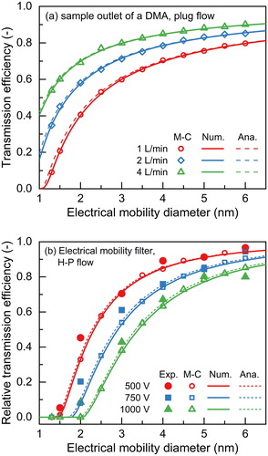
When assumptions 1) – 3) are satisfied in the test conditions, the transmission efficiencies of sub-6-nm charged nanoparticles estimated using the simplified numerical model and the simplified model agree well with those from the Monte Carlo method for both the DMA sample outlet and the EMF (Figure 4). For instance, the mean and maximum absolute differences between the transmission efficiencies for a half-mini DMA sample outlet (Attoui and Fernández de la Mora 2016; Fernández de la Mora and Kozlowski 2013) estimated using the analytical model and the Monte Carlo method are 0.8% and 4.1%, respectively. Good agreement between the models and the measured transmission efficiency was also observed for the EMF. The mean absolute difference between the transmission efficiencies estimated using the analytical model and the measured efficiencies for the EMF is 4.0%, while the mean relative standard deviation of the measured efficiencies themselves is ∼7.2% (Surawski et al. 2017). The difference of 4.0% is comparable to the mean absolute residue (3.7%) of the semi-empirical formula with four additional fitted empirical parameters used by Bezantakos et al. (2015).

Figure 4. Transmission efficiencies of charged particles through (a) the sample outlet of a differential mobility analyzer and (b) an electrical mobility filter. (a) a = 0.1 m, L = 0.04 m, b = 0.16 m, R = 2 mm, and U₀ = -300 V; (b) a = 0.05 m, L = 0.035 m, L₂ = 0.01 m, L₃ = 0.195 m, b = 0.05 m, R = 3.2 mm, and Q = 1.5 L/min. In (b), the transmission efficiencies are shown in relative values for comparing with the experimentally determined efficiencies. The relative transmission efficiency of an electrical mobility filter is the ratio of the transmission efficiency through the adverse field to its corresponding efficiency when no high voltage is applied. The measured relative transmission efficiencies in (b) are from Surawski et al. (2017). The air flow is assumed to be the plug flow and the Hagen-Poiseuille flow (H-P) in (a) and (b), respectively. Exp, M-C, Num, and Ana in the figure legends are abbreviations for experiments, Monte Carlo method, simplified numerical model, and simplified analytical model, respectively.

However, the assumptions for the simplified numerical model and the simplified model may sometimes be violated in the various conditions of real applications. Thus, the following discussion will be mainly focused on validity of the two proposed models under these unfavorable conditions, i.e., a long adverse electric field with respect to the entire tube, a short electric field with respect to the tube radius, and a short tube length before the adverse electric field compared to the entrance length of air flow. These three conditions correspond to the violation of assumptions 3), 2), and 1), respectively. The following tests are based on the DMA sample outlet and their findings are also valid for the EMF.

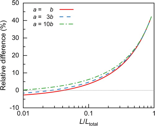
According to assumption 3), the simplified analytical model may deviate from the true transmission efficiency when the diffusion loss inside the adverse field contribute majorly to the diffusion losses in the entire tube. To verify this, particle transmission through a long electric field with respect to the entire tube (L = 0.2 m, a = b = 0.01 m) is tested, as shown in Figure 5. Under this condition, a large discrepancy was found between the simplified analytical model and the Monte Carlo method, whereas the simplified numerical model agrees with the Monte Carlo method because it does not rely on assumption 3). The discrepancy between the simplified analytical model and the Monte Carlo method increases with the increasing ratio of L to L_total. For instance, the relative bias of the simplified analytical model is less than ∼5% when L/L_total < 0.1 in the test conditions (Figure 6). It should be clarified that the value of this bias is also dependent on L_total, hence, although L/L_total is larger than 0.1 for results given in Figure 4 of this study and Figure 5 of Cai, Zhou, and Jiang (2019), relatively good agreements were also observed. The rough estimation of assumption 3) limits the validity of the simplified analytical model. However, it can still be applied as a fast and straightforward solution when the L is short compared to L_total, e.g., the EMF in Bezantakos et al. (2015) and Surawski et al. (2017) and the sample outlet of the half-mini DMA (Cai, Zhou, and Jiang 2019).

Figure 5. Transmission efficiencies of charged particles through a sample outlet of a differential mobility analyzer with a long adverse electric field with respect to the total tube length. a = b = 0.01 m, L = 0.2 m, b = 0.16 m, R = 2 mm, d_p = 1.5 nm, and Q = 2 L/min. ξ is the dimensionless parameter characterizing the electrostatic losses. H-P, M-C, Num, and Ana in the figure legends are abbreviations for Hagen-Poiseuille, Monte Carlo method, simplified numerical model, and simplified analytical model, respectively.

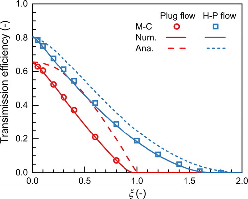
Figure 6. The relative difference between the simplified analytical model and the simplified numerical model for the sample outlet of a differential mobility analyzer. L_total = a + L + b = 0.2 m, R = 2 mm, Q = 2 L/min, d_p = 1.5 nm, and ξ = 0.5. The flow is assumed to be the Hagen-Poiseuille flow.

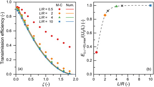
When the electric field is short with respect to the tube radius, the radial displacement of particles may occur within a non-negligible axial length (Tammet 2015) and this may increase the uncertainty of the modeled particle diffusional loss inside the electric field. As shown in Figure 7a, the transmission efficiency of particles predicted by the Monte Carlo method increases significantly when L/R decreases below 4, whereas the simplified numerical model does not follow this increase. However, the main cause of the underestimation of transmission efficiency when using the simplified numerical model at L/R < 4 is the axial intensity of the adverse electric field rather than the effect of electric field on particle diffusion. The numerical and simplified analytical models are proposed based on E_x(xmid,r) = U₀/L, which is found to be valid when L/R ≥ 4 (Tammet 2015). When L/R < 4, E_x is smaller than U₀/L and, hence, the true adverse electrical migration velocity of particles (Z·E_x) is smaller than that assumed in the numerical and simplified analytical models. As a result, the transmission efficiency is underestimated in the numerical and simplified analytical models when L/R < 4. The results in Figure 7 indicate that assumption 2) does not cause a significant bias in the estimated transmission efficiency as long as E_x(xmid,r) = U₀/L, i.e., L/R ≥ 4.

Figure 7. The comparison between the simplified numerical model (Num) and the Monte Carlo method (M-C) at short electric field lengths inside the sample outlet of a differential mobility analyzer. The flow is assumed to be the Hagen-Poiseuille flow. a = b = 0.01 m, R = 2 mm, Q = 2 L/min, d_p = 1.5 nm. (a) Particle transmission efficiency. (b) The normalized maximum axial electrical field, E_(x,r=0),max as a function of L/R. When the adverse electric field is uniform in the middle of the adverse electric field (x = a + L/2), E_(x,r=0),max is equal to U₀/L. The same markers in (a) and (b) correspond to the same L/R value, while other L/R values in (b) are shown in asterisk markers (*).

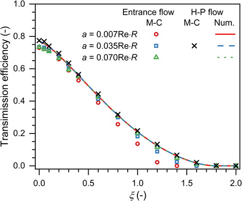
In real applications, the flow field is sometimes not the ideal Hagen-Poiseuille flow or plug flow. For instance, the length before the adverse electric field of the EMF in Bezantakos et al. (2015) is shorter than the entrance length. If the tube upstream the EMF is also short so that a is smaller than the entrance length, L_entrance, the flow profile may not be fully developed at the entrance of the electric field. L_entrance is approximately equal to 0.1Re·R (Bergman et al. 2011), where Re is the Reynolds number. Figure 8 compares the transmission efficiencies through the entrance flow and the Hagen-Poiseuille flow at different values of a which are smaller than L_entrance. It was found that when a is smaller than L_entrance, the transmission efficiency is overestimated using the idealized Hagen-Poiseuille flow field, especially for a strong adverse electric field (large ξ). This is because particles migrate toward the axis in the entrance region. If a is smaller than L_entrance, a fraction of particles that can finally migrate inside r_ξ at x > L_entrance remain outside r_ξ at x = a (see Figure 2a) and they are thus scavenged due to the radial and adverse axial electric fields. In addition, r_ξ is found to be a function of a for a < L_entrance. Note that even without the electric field (ξ = 0), the diffusional loss for the entrance flow is larger than that for the Hagen-Poiseuille flow. However, whether or not to consider the entrance flow effect does not appear to cause a large deviation when ξ < 1 unless a is much smaller than L_entrance (e.g., a < 0.01Re·R). For instance, when a = 0.035Re·R and ξ < 1, the maximum absolute and relative differences for the transmission efficiency in Figure 8 are 3.6% and 7.5%, respectively. Note that a larger a (e.g., a > 0.01Re·R) would be needed to reduce the relative difference when ξ > 1.

Figure 8. The influence of entrance flow on the transmission of charged particles through the adverse electric field. The entrance length is approximately 0.1Re·R, where Re is the Reynold number. H-P, M-C, and Num in the figure legends are abbreviations for Hagen-Poiseuille, Monte Carlo method, and simplified numerical model, respectively. L = 0.05 m, b = 0.1 m, R = 2 mm, Q = 2 L/min, d_p = 1.5 nm, and 0.07Re·R is approximately 0.1 m.

4. Conclusions

A simplified numerical model and a simplified analytical model are proposed for estimating the transmission efficiency of charged nanoparticles and ions through an adverse axial electric field. Particle losses due to diffusion and electrostatic migration are both considered. The adverse electric field is assumed to be radially uniform in the middle of the electric field (x = a + L/2). The radial electric field at the entrance and exit of the adverse electric field is approximately symmetric. The air flow profile is assumed to be uniform (the plug flow) or follow the Hagen-Poiseuille profile. A Monte Carlo method based on single trajectory particle tracking was used as the benchmark. The simplified numerical model agrees with the Monte Carlo method unless the electric field is too short (L/R < 4) to be radially uniform in the middle of the electric field or the tube length before the electric field is much shorter than the entrance length of the air flow. In addition to the above conditions, the simplified analytical model is valid when the adverse electric field is relatively short compared to the total tube length. If the assumptions in developing the proposed models are significantly violated, the Monte Carlo method which requires higher computational expenses can be used instead to estimate the transmission efficiency. Both the proposed models and the Monte Carlo method were applied for an electrical mobility filter and the sample outlet of a differential mobility analyzer. Under the typical conditions for these devices, the transmission efficiency estimated using the proposed models agrees well not only with the Monte Carlo method (a mean absolute difference smaller than 1%) and but also with the measured transmission efficiencies for sub-6 nm particles.

Code availability

The MATLAB codes for the simplified analytical and numerical models are included in the supporting information. The Julia codes for the Monte Carlo model and the electric field are available upon request.

Acknowledgment

The authors thank Prof. Hannes Tammet at the University of Tartu for sharing his codes for numerically solving the flow field and the electric field, Prof. Zeyu Mao at Tsinghua University for the discussion on the simplified numerical model, and the anonymous reviewers of Cai, Zhou, and Jiang (2019) for their valuable comments that inspired further analysis reported in this study.

Additional information

Funding

Financial support from National Key R&D Program of China (2017YFC0209503) and the National Natural Science Foundation of China (21876094) are acknowledged.

References

- Attoui, M., and J. Fernández de la Mora. 2016. Flow driven transmission of charged particles against an axial field in antistatic tubes at the sample outlet of a differential mobility analyzer. J. Aerosol Sci. 100:91–96. doi:10.1016/j.jaerosci.2016.06.002.
- Bergman, T. L., A. S. Lavine, F. P. Incropera, and D. P. DeWitt. 2011. Fundamentals of heat and mass transfer. Hoboken, NJ: John Wiley & Sons, Inc.
- Bezantakos, S., L. Huang, K. Barmpounis, M. Attoui, A. Schmidt-Ott, and G. Biskos. 2015. A cost-effective electrostatic precipitator for aerosol nanoparticle segregation. Aerosol Sci. Technol. 49 (1):iv–vi. doi:10.1080/02786826.2014.1002829.
- Cai, R., J. Jiang, S. Mirme, and J. Kangasluoma. 2019. Parameters governing the performance of electrical mobility spectrometers for measuring Sub-3 nm particles. J. Aerosol. Sci. 127:102–115. doi:10.1016/j.jaerosci.2018.11.002.
- Cai, R., Y. Zhou, and J. Jiang. 2019. Transmission of charged nanoparticles through the DMA adverse axial electric field and its improvement. Aerosol Sci. Technol. (published online). doi:10.1080/02786826.2019.1673306.
- Fernández de la Mora, J., and J. Kozlowski. 2013. Hand-held differential mobility analyzers of high resolution for 1–30nm particles: Design and fabrication considerations. J. Aerosol Sci. 57:45–53. doi:10.1016/j.jaerosci.2012.10.009.
- Franchin, A., A. Downard, J. Kangasluoma, T. Nieminen, K. Lehtipalo, G. Steiner, H. E. Manninen, T. Petäjä, R. C. Flagan, and M. Kulmala. 2016. A new high-transmission inlet for the Caltech nano-RDMA for size distribution measurements of Sub-3 nm ions at ambient concentrations. Atmos. Meas. Techniques 9 (6):2709–2720. doi:10.5194/amt-9-2709-2016.
- Fu, Y., M. Xue, R. Cai, J. Kangasluoma, and J. Jiang. 2019. Theoretical and experimental analysis of the core sampling method: reducing diffusional losses in aerosol sampling line. Aerosol Sci. Technol. 53 (7):793–801. doi:10.1080/02786826.2019.1608354.
- Gormley, P. G., and M. Kennedy. 1949. Diffusion from a stream flowing through a cylindrical tube. Proc. Roy. Irish Acad.. Section A: Math. Phys. Sci. 52:163–168.
- Knutson, E. O., and K. T. Whitby. 1975. Aerosol classification by electric mobility: Apparatus, theory, and applications. Aerosol Sci. Technol. 6 (6):443–451. doi:10.1016/0021-8502(75)90060-9.
- Surawski, N. C., S. Bezantakos, K. Barmpounis, M. C. Dallaston, A. Schmidt-Ott, and G. Biskos. 2017. A tunable high-pass filter for simple and inexpensive size-segregation of Sub-10-nm nanoparticles. Sci. Rep. 7 (1):45678. doi:10.1038/srep45678.
- Tammet, H. 1970. The aspiration method for the determination of atmospheric-ion spectra. Jerusalem: Israel Program for Scientific Translations.
- Tammet, H. 2015. Passage of charged particles through segmented axial-field tubes. Aerosol Sci. Technol. 49 (4):220–228. doi:10.1080/02786826.2015.1018986.
- Targ, S. M. 1951. Basic problems of the theory of laminar flows (in Russian). Moscow: Gostehizdat.