Multiparametric optical characterization of airborne dust with single particle extinction and scattering

Abstract

We describe a robust, portable, deployable instrument for multiparametric optical characterization of single airborne particles. It is based on the Single Particle Extinction and Scattering method with additional sensors at 45° and 90° angles. Four independent optical parameters are associated to each particle. Basically, it provides a rigorous measurement of the extinction cross section and the complex amplitude of the forward scattered field. Moreover, thanks to the multiparametric single particle approach, it is possible to roughly classify the particles within a size range from a few hundreds of nanometers to some micrometers. By assigning a reasonable single scattering albedo for each population, our data are enough to fit the phase function with acceptable uncertainties. We report here the results of tests performed with water droplets, generating well controlled data without any free parameters. Data analysis is described in detail. We also report measurements performed on urban aerosol collected in the city of Milan by recovering the optical properties and feeding radiative transfer models. The findings reported here support the importance of an accurate measurement of the phase function, as already established by the Community.

Copyright © 2020 American Association for Aerosol Research

EDITOR:

• Hans Moosmüller

1. Introduction

Liquid and solid particles suspended in the atmosphere strongly influence the transfer of radiant energy and, in turn, weather and climate. Aerosol particles interact with solar radiation through absorption and scattering, and with terrestrial radiation through absorption, scattering and emission (Chylek and Coakley 1974). Particles of both natural and anthropogenic origin play an important role in atmospheric chemistry and biogeochemical cycles (Stocker et al. 2014).

Eolian mineral dust aerosol (hereinafter “dust”) represents an important component of the climate system (Stocker et al. 2014) and plays a key role in biogeochemical cycles (Mahowald et al. 2010). Fine mineral dust particles (<10 μm diameter) deflated from natural and/or anthropogenic continental sources and entrained in the troposphere is believed to exert a significant short-wave and long-wave radiative forcing (Albani et al. 2014; Stocker et al. 2014). The amplitude of this forcing is related to some key variables such as aerosol optical depth and altitude of the dust layer, as well as size, shape and mineralogy of dust grains (Dubovik et al. 2002).

In this work, we describe a novel instrument based and expanding on the recently introduced Single particle Extinction and Scattering (SPES) optical method (Potenza, Sanvito, and Pullia 2015). Its goal is to characterize the relevant parameters needed for radiative transfer computations from measurements of airborne particles. Working on single-particles guarantees to be independent of any inversion problem and allows statistical approaches on raw data that are impossible for other methods.

The instrument is a portable, deployable, stand-alone device capable of operating outdoors under extreme conditions. It has been designed, assembled and tested for working within a temperature range of approximately −30 °C to +50 °C. Moreover, the mechanics have been designed in such a way to ensure good stability whenever moving the instrument during the operations, including packing, unpacking, handling and shipping. The device pumps air from the environment at a flow of a few dm³min⁻¹. It works in continuous, storing raw data in an internal memory, accessible through a LAN connection.

In Section 2, we briefly describe the optical scheme adopted for the measurements and the air adduction system. Section 3 is devoted to the detectors and the acquisition system, which has been specifically designed, realized and tested for this application. Section 4 is dedicated to explaining the strategy for handling raw data and the physical basics of the method for obtaining the relevant parameters. In Section 5, we present some examples of experimental data obtained with aerosol suspensions, populated by micron-sized, polydisperse, pure water droplets and by atmospheric dust collected under different conditions. Data analysis is explained in detail and the impact of results on radiative transfer models is briefly discussed. Finally, conclusions are outlined in Section 6.

2. The instrument

The instrument described here relies on direct-hand experience accumulated over almost a decade with the SPES instruments developed for measuring liquid suspensions. It is basically the standard SPES, with two additional sensors and some changes aimed at operating in the environment. Relying on a self-reference interferometric scheme, it provides a direct measurement of the complex field scattered in the forward direction by single particles crossing a tightly focused laser beam. The intense transmitted beam and the fainter scattered field superimpose and interfere on a four-quadrant photodiode placed in the far field of the beam waist. Let us consider a particle passing through the focal region along its diameter. By the conservation of power, when it crosses the center of the focal spot it will depress the transmitted beam, removing power by scattering and absorption. This power balance can also be interpreted in terms of the Optical Theorem (or Extinction Theorem) as a consequence of the destructive interference between the two waves (Van de Hulst 1981; Bohren and Huffman 2008; Newton 1976; Potenza et al. 2010). This depression rigorously gives a precise measure of the extinction cross-section, $C_{\mathit{ext}}.$ When a particle within the focal region is located out of the optical axis, the two emerging wavefronts are slightly skewed, and the intensity modulation produced by interference is proportional to the amplitude of the forward scattered field. The segmented sensor then provides a differential measure of the intensity modulations due to interference, thus assigning the real and imaginary part of the forward scattering field amplitude as detailed in (Potenza, Sanvito, and Pullia 2015). A similar modulation occurs in case the particle does not cross the beam waist diametrically: interference between skewed wavefronts produces additional asymmetry in the transmitted beam intensity distribution. This can be quantified and is directly related to the off-axis distance as an intrinsic validation tool to select events generated by particles crossing the beam at a given selectable distance from the optical axis. Finally, the continuous measurement of the current generated by the transmitted beam – unaffected by particles most of the time – gives a real-time monitoring of the laser power. Each self-referenced signal is translated into a relative information about the particle, thus making the SPES raw data rigorously calibration free. Two additional sensors are placed at 45 and 90 degrees with respect to the optical axis, in order to gain further insight into the angular dependence of scattering from airborne particles. A schematic of the optical layout is shown in Figure 1. A laser head (Coherent 635 nm wavelength, 5 mW power) emits a collimated beam with a waist $w=0.2$ mm approximately. The beam is expanded 5 times by a telescope constituted by a negative aspheric doublet (A1: −20 mm focal length) and a positive aspheric doublet (A2: +100 mm focal length). A 50 mm doublet (A3) focuses the beam into the scattering region down to a waist w₀ = 12 µm. The diverging beam is collected 60 mm downstream by a quadrant photodiode (QPD) sensor 8 mm in diameter, after being attenuated by an OD0.3 neutral filter (N). Notice that the laser beam is always collimated along the optical path, except for the focusing into the scattering region, thus making it unaffected by the precise positioning of the optical elements. This is relevant in case of maintenance: parts of the setup can be replaced without affecting the collimation of the entire system. This also ensures that there are no focal spots along the optical path other than the scattering volume, preventing the possibility of fake events. The only element that needs precise positioning is the scattering cell, to deliver the air flux through the laser beam focal region. All the system components are fixed onto a rail that reduces to a minimum any thermal deformation. All these features make the system very robust and suitable for being moved, delivered, repositioned and operated even in extreme environments for long term measurement campaigns. The instrument weights about 10 kg and is contained in a 450 × 310 × 130 mm steel enclosure. Power consumption is ∼12 W, in addition to a ∼10 W air pump for withdrawing air inside the cell. The instrument includes a cooling system for the laser and the power supply; otherwise it operates at ambient temperature. In case, a proper heating or drying system for the airflow can be connected to the inlet in the top cover. A system unit currently operating in Antarctica, at Concordia station, includes a heating system to ensure the air entering the chamber is at approximately standard room temperature in addition to drying the particles. As regards the instrument in the urban setting, we did not apply any heating/drying system in order to study the aerosol as it is in the atmosphere.

Figure 1. Schematic of the optical layout. The 635 nm wavelength laser beam is expanded and focused into the flow cell, where particles are driven through its focal region. The air flow (∼dm³min⁻¹) is perpendicular to the beam, the air inlet is indicated with a circle in the figure. The emerging beam is collected in the forward direction by the QPD. Light power scattered toward the elliptical mirror in the lower part of the flow cell in this drawing is collected by the P90 sensor. The collection solid angle is 1.2 sr. The light scattered toward the P45 sensor is collected directly within a solid angle of about 0.01 rad.

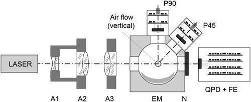
The air adduction system has been designed to properly deliver dust through the laser focal spot. A sheet-shaped air flow with a negligible longitudinal extension with respect to the focal depth is generated between two nozzles. The flow conditions between these two nozzles have been preliminary investigated through numerical simulations. A steady state flow analysis has been performed, by enforcing the experimentally measured suction flowrate of the pump, and a static relative pressure at the air inlet with zero velocity gradient. Smooth walls have been considered. The turbulence has been modeled by the Menter’s Shear Stress Model (Menter 1994), using a very fine mesh at the walls (8 mesh prismatic layers). The simulation shows that the air strip has an inner part with a nearly uniform velocity and almost constant thickness, and has a negligible transversal divergence. The air speed at the measurement position is estimated to be ∼10 ms⁻¹. According to the beam waist, this gives a typical transit time of several µs, which is in accordance with the experimental data.

The flow cell is milled from an Aluminum block. It has four optical viewports: two for the transilluminating beam, one for the 45° and one for the 90° scattered light power (P90 and P45). The 90° scattered light is collected over a wide solid angle (1.2 sr) by an elliptical mirror (EM) specifically designed and custom built. The two foci of the mirror are at the laser focal spot and slightly beyond the sensor position, respectively; the reflected light passes through the cell and impinges onto the sensor on the opposite side (in the upper part of Figure 1). The angle detectors are still QPDs 8 mm in diameter where all the four cathodes are connected together. This choice is simply dictated by the ease of finding large enough sensors and by the uniformity of the front-end electronics. Detectors collecting light at 45° and 90° do not require a very precise alignment, both in transversal and longitudinal positions. Their calibration is limited to one numerical constant each, which is applied for all the events throughout the entire sensitivity window. By contrast, while not requiring any calibration, the forward QPD detector must be precisely positioned with its center along the optical axis; a x–y micrometric translation stage has been used to this purpose. Conversely, the longitudinal positioning is not demanding, the SPES interference patterns being homothetic functions as discussed in literature (Potenza, Sanvito, and Pullia 2015).

3. Detectors and acquisition system

The front-end (FE) electronics are detailed in previous works (Pullia et al. 2012). In the forward direction, they consist of four hybrid circuits, one for each photodetector in the QPD. Detectors at angles 45° and 90° consist of one hybrid circuit each. The FE circuits are low noise current preamplifiers, that split the continuous, intense current (dc component) and the fast, faint current fluctuations (ac component) into two different channels. The photocurrent is integrated over a time longer than the transit time, thus giving a measure of the dc current, and an opposite current is generated and added to the raw photocurrent. In such a way, each FE circuit provides two voltage signals: the former gives the fast, zero-averaged ac fluctuation, namely, the signal fluctuation induced by the particle passing through the beam, while the latter provides the continuous monitoring of the impinging beam power. As a result, the fast ac fluctuations can be digitized properly through a device with relatively limited dynamics, given the very small power fluctuations upon the transmitted beam induced by the particles to be measured here (of the order of 10⁻⁴). The same approach is adopted for the angle photodetectors to drastically reduce the effects of the unavoidable straylight from the main beam: this continuous contribution can be much higher than the small scattered power. The FE electronics produce zero-averaged signals to be delivered to the digitizer. A sampling rate of 10 MHz has been adopted, tuned to the bandwidth of the FE electronics, B = 5 MHz.

The noise level guaranteed by the FE amplifiers is well below the minimum laser noise. The presence of structured optical noise (random telegraph signal, RTS, see Sanvito et al. 2013), typical of semiconductor junctions, constitutes the main limitation to the sensitivity of SPES measurements. Fake trigger events may be generated by laser noise, so that the trigger level must be set above a given threshold. The laser adopted here represents a good compromise in this respect.

The system is operated under conditions such that the shot noise is well below the required sensitivity. In our case, shot noise must be carefully considered, since the forward detectors are continuously impinged by a relatively high optical power, upon which particles impose very small, fast fluctuations. The intensity has been tuned in such a way that the a dimensional fluctuations, i.e., the shot noise divided by the main beam, are about 2.5·10⁻⁴. In the absence of laser noise, this would be enough to accurately detect particles of a few hundreds of nm in diameter.

Voltage signals from the FE electronics are delivered to the custom acquisition system. It has been specifically designed to be flexible and reconfigurable in view of extreme, non-laboratory working conditions. Moreover, custom trigger procedures can be implemented, in order to highly reduce the amount of data to be stored in (and transferred from) remote regions with limited data transfer capacity.

The system is composed of an embedded system and two custom made electronic boards. The signals from the six FE electronics are sent to the custom boards with four independent channels each, for real time, synchronous monitoring of the signals at 10 MHz sampling rate. Each board is equipped with a FPGA that permits hardware execution of real time data analysis to optimize the trigger performance. Each board includes both an internal and an external trigger, so that the trigger can be switched from one to the other as necessary.

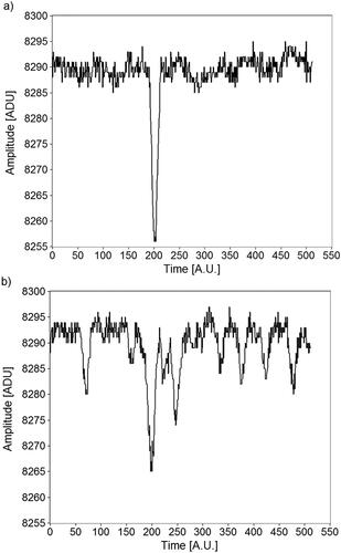
Each signal from the FE electronics is delivered to a dedicated 14-bit dynamics ADC. Digital output from the ADC is processed by the FPGA and the data sequence is stored into a 512 × 14 words temporary buffer. Trigger operations are performed by the FPGA on the incoming streaming data. Their flexibility allows the user to program and adapt trigger operations even after integration and installation of the instrument. In view of this specific SPES application, the aim is to trigger signals with very small fluctuations from the offset (even after the dc subtraction operated by the FE electronics). This poses two critical limitations: (1) the offset can slightly change due to environmental conditions (for example temperature), thus actually changing the effective trigger threshold; (2) any kind of noise can affect signals and generate fake trigger events. To overcome the former issue, hardware has been specifically designed. For the latter, a software solution has been adopted on the acquired data, as described in the next section. FPGAs have been programed to evaluate the offset level in quasi-real time by averaging 128 samples and to reset the trigger threshold accordingly (offset follower). It must reject averages coming from data sets with non-constant offsets. An estimate of the signal quality is achieved by simply averaging the absolute displacements of the same 128 samples from the average. An example of two data sets is shown in Figure 2. A statistical analysis of the typical fluctuations in the real environment allowed us to set a “quality threshold” to prevent trigger resetting when the offset value comes from noisy signals. By contrast, whenever the offset follower returns a smooth enough signal, the trigger is updated by applying the trigger threshold to the current offset level. These operations are asynchronous with the trigger and are performed in real time on the data stream, providing results within 8 μs.

Figure 2. Examples of the raw data entering the asynchronous procedure to perform the offset follower. (a) Conditions of limited noise, with an average discrepancy 1: the trigger reset is active, and the trigger level is updated. (b) Noise conditions, with an average discrepancy 5: reset is prevented.

Two trigger operation modes are currently possible for continuous measurements, although the system remains fully reconfigurable.

3.1. Differential trigger

As mentioned above and evidenced in past works, SPES method is mainly limited by laser instabilities. Since the main source of noise is the laser itself, exploiting the synchronous detection from the four QPD sensors it is possible to significantly reduce noise by evaluating differences of signals from different segments. To overcome laser disturbances, a configurable set of differences is possible. Unfortunately, unlike the results so far obtained in the laboratory, in Antarctica an uncorrelated noise is present among the different channels, appreciably limiting the benefits introduced by working in differential mode.

3.2. Filtered trigger

We exploit the signals from the P90 sensor to operate an effective trigger which guarantees a stable threshold and the maximum dynamics for the signals, stable as well. In order to push further the trigger quality, we split the 90° scattering signal into two equal signals. The former is passed through a 1 MHz passive filter to further reduce the noise fluctuations and is used for triggering. The latter is sent to the ADC. This is the operation mode operating in Antarctica at the time of writing, during austral summer and fall seasons 2019.

The board generating the trigger event also provides an external trigger signal to the other board and the embedded system, in order to download data from both buffers simultaneously and read some additional parameters. A latency of less than 50 ns is present between the data from the two boards, which is small enough for our purposes, provided that the 4 QPD signals are collected by one board. The embedded system also contains a FPGA that takes in charge data collection and transfer from the two boards to the microprocessor. This manages slow control operations such as dc monitoring, readout of environmental parameters, LAN, FTP server and UDP I/O connections.

Before entering the ADC, the signals detected from the QPD are treated in such a way that the 2¹⁴ levels optimimize the dynamical range with the maximum sensitivity to small fluctuations. With a dc current of the order of 30 μA from each QPD segment, the relative shot noise fluctuations are of the order of 3·10⁻⁴. With a maximum level of 1.6 V, the 14 bits ADU is 1.95·10⁻⁴ V, which corresponds to a relative fluctuation of 4·10⁻⁴. As a result, the dynamical range spans a factor >1000, which is more than enough for our purposes. Finally, this level is compatible with the shot noise (see above).

4. Data reduction and analysis

Raw data are reduced and analyzed through a dedicated software imposing constraints and checking for strict conditions about specific features of the signals. Well-behaved signals are recognizable through a sequence of template matching procedures. After this process, each selected event can be associated with a quality figure, that can be useful in further statistical analysis.

More precisely, raw data are passed through a three-step procedure. (1) A preliminary data reduction is performed to get rid of noise generated signals, mainly due to laser fluctuations and electronics. (2) A software trigger is implemented on the pre-selected data. The high sampling frequency allows for accurate pulse shape analysis. Moreover, at this step we get rid of spurious events, such as events generated by particles passing through the beam out of ideal conditions (Potenza, Sanvito, and Pullia 2015). (3) Selected events are finally passed to the data analysis procedure, that extracts the optical parameters of each measured particle. Here we recall the basics of the SPES analysis and give some additional details on how the information delivered by the 45° and 90° detectors is handled. Finally, we discuss how to extract the optical parameters to feed radiative transfer models.

As shown in previous works (Potenza, Sanvito, and Pullia 2015; Mariani et al. 2017), the SPES measurement directly provides the adimensional complex field amplitude, $S\left(0\right),$ scattered in the forward direction by each particle (Van de Hulst 1981; Bohren and Huffman 2008). For the sake of clarity, $S\left(0\right)$ is a complex number defined in such a way that the field $E_S$ scattered in the direction $\theta ,\phi$ at a distance $R$ from a particle illuminated by an incoming field $E_i$ with wavelength $\lambda$ and $k=2\pi /\lambda$ is: (1) $$E_S=\frac{e^{\mathit{ikR}}}{\mathit{ikR}}S\left(\theta ,\phi \right)E_i$$(1)

We introduce the adimensional flux ${F\left(\theta ,\phi \right)=\left|S\left(\theta ,\phi \right)\right|}^2.$ Generally speaking, $F\left(\theta ,\phi \right)$ rigorously gives the phase function $p\left(\theta ,\phi \right)$ once normalized by the total scattering cross section, $C_{\mathit{sca}},$ and divided by $k^2.$ Since the SPES method works on the forward scattered wavefront, it does not allow to recover this piece of information. However, additional sensors at 45° and 90° measure integrals of the adimensional flux over given solid angles. Each particle is then associated with four independent parameters measured simultaneously, hence with the same particle orientation and illumination conditions.

We represent SPES data in terms of two quantities directly related to the real and imaginary parts of the scattering amplitude measured by SPES: the extinction cross section, $C_{\mathit{ext}},$ namely the ratio between the power removed from the incoming beam and its intensity, and the optical thickness of the particle, defined below. Notice that, by the Optical Theorem (Van de Hulst 1981; Bohren and Huffman 2008; Newton 1976; Potenza et al. 2010), $C_{\mathit{ext}}$ is simply proportional to the real part of the forward scattered field amplitude, $\mathit{ReS}\left(0\right),$ which we measure directly with SPES. The optical thickness is defined as the average over the geometrical cross section of the product of the particle refractive index, $m-1,$ and the average geometrical thickness of the particle in the illumination direction (Van de Hulst 1981). Following (Villa et al. 2016), the physical quantity measured by SPES is $\rho =\tau k,$ where $k=2\pi /\lambda$ and λ is the wavelength, while $\tau =⟨\tau \left(x,y\right)⟩$ is the average optical thickness. Notice that the same approach can be extended to non-spherical and/or non-homogeneous particles, as detailed in (Potenza, Sanvito, et al. 2016; Potenza et al. 2017). Data representation will therefore be provided by assigning one pair ($C_{\mathit{ext}},\mathrm{ }\rho$) to each measured particle. A two-dimensional (2 D) histogram is then obtained collecting events falling into 2 D bins (by adopting a logarithmic scale for convenience).

As clearly shown in previous works, inverting data is not trivial: it is possible to assign a particle size univocally to a given pair ($C_{\mathit{ext}},$ $\rho$) for spheres only. This is due to the several parameters affecting light scattering, such as size (by far the most important, especially in the size range of interest here), composition, internal structure, shape and orientation (Mishchenko, Hovenier, and Travis 2000; Villa et al. 2016; Potenza et al. 2017; Simonsen et al. 2018). We therefore avoid such inversion, except in exceptional cases of samples characterized by spherical particles, basing the analysis on raw optical data instead. Knowing four independent parameters gives access to important information in addition to that obtainable with traditional single particle methods (Ruth 2002; Walser et al. 2017). Moreover, performing statistical analysis on the SPES data sets gives insight into the optical properties of the entire population without the need of ill-posed inversion problems as it is the case of traditional multi-particle methods.

Measuring $S\left(0\right)$ provides additional information. We can rigorously access the forward scattered intensity through the forward scattered adimensional flux,$\mathrm{ }{F\left(0\right)=\left|S\left(0\right)\right|}^2.$ It should be emphasized that this result is all but trivial and is made possible by the specific ability of SPES to measure the amplitude at exactly zero-angle. As clearly discussed in (Van de Hulst 1981), with traditional optical methods one cannot accurately separate the incoming and scattered radiation in the forward direction, so that the only way is to extrapolate the intensity from small angle light scattering measurements (truncation effect). This limitation is overcome by the self-reference interferometric approach (see Potenza et al. [2010] and [2015] for further details).

Let us consider the total power $P_S$ scattered at an angle $\theta$ within a given solid angle $\Omega .$ Dividing it by the incoming total power, $P_i,$ we attain a quantity that only depends on the average $F\left(\theta ,\phi \right)$ over the solid angle $\Omega$ and the incoming beam size. By assuming a Gaussian beam transversal profile (as it is in our case) with a beam waist $w_0,$ we have: (2) $$r=\frac{P_S}{P_i}=\frac{2}{k^2}\frac{\int F\left(\theta ,\phi \right)d\varpi }{{\pi w}_0^2}$$(2) where $d\varpi =\hspace{0.17em}\text{sin}\hspace{0.17em}\mathit{\text{θdθdφ}}$ is the element of solid angle. Since in our instrument $w_0$ is well known, and the incoming power is continuously monitored as discussed above, by measuring $P_S$ within a given solid angle we measure the integral of the adimensional flux $\int F\left(\theta ,\phi \right)d\varpi {=\int \left|S\left(\theta ,\phi \right)\right|}^{2}d\varpi$ over the given solid angle $\Omega .$ We will indicate the two measurements at 45° and 90°, as $F\left(45\right)$ and $F\left(90\right),$ respectively.

Our results can be cast in a more general framework, with no dependence on any instrumental parameter, that provides the normalized values of the $p\left(\theta ,\phi \right)$ function integrated over the collection solid angle. The SPES measurement accesses the beam attenuation, rigorously defined as $a=P_E/P_i,$ where $P_E$ is the power removed from the beam through scattering and absorption (if any). According to the Optical Theorem and following (Potenza, Sanvito, and Pullia 2015) we can write: (3) $$a=\frac{P_E}{P_i}=8\frac{\mathit{ReS}\left(0\right)}{k^2{w}_0^2}$$(3) where $\mathit{ReS}\left(0\right)$ is the real part of the forward scattered field amplitude.

The choice of having the same QPD and FE electronics for each sensor causes the instrumental parameters to cancel out rigorously by taking the ratio of $r$ to $a.$ This produces a quantity that solely depends on the scattering and extinction properties of the particle: (4) $$p=\frac{P_S}{P_E}=\frac{1}{4\pi }\mathrm{ }\frac{\int F\left(\theta ,\phi \right)d\varpi }{\mathit{ReS}\left(0\right)}\mathrm{ }=\frac{\int F\left(\theta ,\phi \right)d\varpi }{k^2{C}_{\mathit{sca}}}$$(4) which gives $p\left(0\right),$ $p\left(45\right),$ and $p\left(90\right).$ In the ideal case of purely dielectric particles, since $C_{\mathit{ext}}=C_{\mathit{sca}},$ it rigorously provides the values of the normalized phase function $p\left(\theta ,\phi \right)$ integrated over the collection solid angles. In presence of absorption $C_{\mathit{sca}}=\mathit{ssa}{\mathrm{ }C}_{\mathit{ext}},$ where $\mathit{ssa}$ is, by definition, the single scattering albedo of the particle. If assumptions can be made for $\mathit{ssa},$ an estimate is straightforward from the experimental data for $C_{\mathit{ext}}.$

We are not able to measure the $\mathit{ssa}$ with our instrument and, in general, it cannot be safely assumed for each particle. We therefore cannot directly access this parameter on an experimental basis. Nevertheless, since the specific aim of this work is to assess the optical properties of particles to feed radiative transfer models, we can rely on rough estimates of $\mathit{ssa}$ for a given particle population as currently measured with dedicated instruments (see for example Onasch et al. [2015] and references therein). The SPES method is able to distinguish populations of absorbing and dielectric particles (see below). This reduces the uncertainty on the $\mathit{ssa}$ values for each species — assumed on the basis of independent works — to approximately 5% (Onasch et al. 2015). For instance, estimating $\mathit{ssa}\mathrm{ }=\mathrm{ }0.90$ instead of $\mathit{ssa}\mathrm{ }=\mathrm{ }0.95$ gives an error in the corresponding $p\left(\theta \right)$ value slightly above 5%, that is absolutely acceptable for our goals. We stress that this would not be the case in view of other applications such as, for example, the characterization of the power absorption by the aerosol. In this case the same numbers would give an error of ∼100%.

In conclusion, we rigorously associate each particle with the following parameters: $C_{\mathit{ext}},$ $F\left(0\right),$ $F\left(45\right)$ and $F\left(90\right).$ Notice that these optical parameters are recovered in a very simple way through algebraic operations on raw data for each particle. No inversion or ill-posed fitting or optimization algorithms are required due to the self-reference scheme and the single particle approach. In addition, by analyzing data populations in the ($C_{\mathit{ext}},\mathrm{ }\rho )\mathrm{ }$ plane, exploiting the SPES capabilities allows to access further information on a statistical basis, as detailed in previous works (Potenza, Sanvito, and Pullia 2015, Potenza, Sanvito, et al. 2016; Villa et al. 2016; Potenza et al. 2017; Simonsen et al. 2018). Additionally, we estimate the average value for the $\mathit{ssa}$ of the relevant populations (see below), so as to provide the optical properties of the cloud of measured particles in terms of the average, normalized $p\left(0\right),$ $p\left(45\right)$ and $p\left(90\right),$ $C_{\mathit{ext}},$ and the asymmetry parameter, $g,$ together with the average $\mathit{ssa}.$ These are the parameters needed to feed radiative transfer models.

5. Experimental data

Here we show some examples of experimental data obtained i) from pure water droplets generated with an aerosol generator, whereby to calibrate the angle detectors to accurately check the system and the data reduction and analysis; ii) from airborne particles, collected during preliminary tests in the city of Milan.

Data have been treated as described in the previous section. They are represented by 2 D histograms where the number of events within each 2 D bin is shown in the plane$\mathrm{ }(C_{\mathit{ext}},\mathrm{ }\rho ),$ and in a plot representing $(C_{\mathit{ext}},\mathrm{ }F(0)),$ $\left(C_{\mathit{ext}},\mathrm{ }F\left(45\right)\right)\mathrm{ }$ and $(C_{\mathit{ext}},\mathrm{ }F(90)).$ A relevant part of the collected information is hidden in these plots, although still present in the raw data: for example, the one-to-one correspondence of the parameters measured for each event in the plots, which would require a multi-dimensional representation, and could in principle allow to give much more insight into the optical properties of each measured particle. Nevertheless, we will not enter in such details here, limiting ourselves to a general overview of the data in the representative forms discussed above.

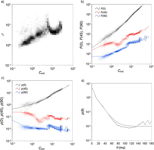
Figure 3 shows typical results obtained under controlled laboratory conditions with spherical, pure water droplets having a diameter within a range from ∼100 nm up to a few microns approximately, generated by a traditional atomizer. It consists of a two-substance nozzle based on the injection principle combined with a baffle placed close to the spray outlet to guarantee a submicron droplet distribution. Droplet size distribution is regulated by the aerosol generator and spans a diameter range up to some microns, which is compatible with what expected measuring in the real environment. This polydisperse sample allows to verify that the instrument behavior (i.e., the calibration constant for the 45° and 90° sensors) is maintained overall the dynamic range, irrespectively of size. We stress that data represented in the $(C_{\mathit{ext}},\mathrm{ }\rho )$ plane, as well as $F\left(0\right),$ are independent of any calibration, since they are obtained from the self-referenced signals collected in the forward direction by the same QPD sensor, which gives two absolute measurements without any free parameter. By contrast, data from the two sensors at 45° and 90° do need calibration to compensate for any possible differences in the collection efficiency of the sensors, the precise calibration of the collection solid angles, and other instrumental parameters such as mirror reflectivity. However, calibration of 45° and 90° channels reduces to one scaling numerical constant each. A number of measurements performed on water droplets have been used to this purpose, while the calibration was based on Mie scattering calculations and proper integrals over the solid angles of the two sensors (solid lines in Figure 3). Notice the non-monotonic behavior caused by peculiar Mie oscillations typical of spheres. Besides the calibration constants, a small correction must be introduced in the small $C_{\mathit{ext}}$ range to compensate for an overestimation of the signals. This is probably attributable to straylight contributions for small particles, due to appreciable scattering power at wide angles. The results shown in Figure 3 are well reproducible: systematic measurements yielded similar outcomes. After this calibration, the measure of water droplets consistently provides results as shown in Figure 3. Notice that peculiar scattering features predicted by Mie oscillations are well visible in the plots in Figure 3, to which we have access because of the large polydispersity of the sample. Specifically, the ripple at about $C_{\mathit{ext}}\mathrm{ }=\mathrm{ }7\mathrm{ }\mathrm{\mu }m2$ is well reproduced by experimental data. These ripples and steps in the $F$ curves represent an absolute, independent accuracy check of both the extinction measurements and the calibration, without any free parameters.

Figure 3. Examples of the results obtained with pure water droplets. Panel (a) represents ${(C}_{\mathit{ext}},\mathrm{ }\rho )$ pairs data as a 2 D histogram, where greytones indicate the relative number of events recorded within the 2 D bin. Panel (b) shows $(C_{\mathit{ext}},\mathrm{ }F(0)),$ $(C_{\mathit{ext}},F(45))$ and $(C_{\mathit{ext}},F(90))$ (from top to bottom), compared to the results of Mie calculations (solid lines). In (c) we report the results obtained for the values of the phase function obtained from (b), compared to the corresponding expected values (solid lines). (d) comparison of the phase functions obtained by fitting experimental data (solid line, black) and through Mie theory for the ensemble of droplets (circles, grey).

Following the approach described above, by referring to Equation (4)(4) $$p=\frac{P_S}{P_E}=\frac{1}{4\pi }\mathrm{ }\frac{\int F\left(\theta ,\phi \right)d\varpi }{\mathit{ReS}\left(0\right)}\mathrm{ }=\frac{\int F\left(\theta ,\phi \right)d\varpi }{k^2{C}_{\mathit{sca}}}$$(4) and by considering the non-absorbing properties of water at our wavelength, we can safely set $\mathit{ssa}\mathrm{ }=\mathrm{ }1$ and rigorously recover the normalized $p\left(0\right),$ $p\left(45\right)$ and $p\left(90\right)$ for each droplet. As mentioned previously, we stress that this result is particularly robust, since it is obtained as the ratio of $r$ and $a$ in Equations (2)(2) $$r=\frac{P_S}{P_i}=\frac{2}{k^2}\frac{\int F\left(\theta ,\phi \right)d\varpi }{{\pi w}_0^2}$$(2) and (3)(3) $$a=\frac{P_E}{P_i}=8\frac{\mathit{ReS}\left(0\right)}{k^2{w}_0^2}$$(3) , hence it does not depend on any instrumental parameter. In Figure 3c we report the results compared to the expected values for the water droplets, obtained following the same approach for the solid curves in Figure 3b. By averaging the values of $p\left(\vartheta \right)$ over the entire population, we find: $$p\left(0\right)=4.75, p\left(45\right)=0.108,\mathrm{ }p\left(90\right)=0.0122$$

We recover an estimate of the phase function $p\left(\vartheta \right)$ associated to the entire particle population by fitting to experimental data a smooth function which describes the main features of the phase function. Moreover, an additional constraint is imposed by the unit integral over the entire solid angle, since $p\left(\vartheta \right)$ is normalized. More specifically, we fit data with the sum of a gaussian, an exponential decay and a constant: (5) $$p\left(\vartheta \right)=\mathit{Aexp}\left[-{\vartheta }^2/2{\sigma }^2\right]+\mathit{Bexp}\left[-\vartheta /b\right]+C$$(5) where $A=p\left(0\right)-p\left(90\right)-B,$ $B=0.25$ and $C=p\left(90\right),$ $\sigma =0.08$ rad, $b=0.25$ rad.

Together with the average $C_{\mathit{ext}}=\mathrm{ }6.43$ μm², rigorously measured through SPES, and $\mathit{ssa}\mathrm{ }=\mathrm{ }1,$ this is all what is needed to feed the radiative transfer models.

In this particular case, the spherical shape of the droplets and the known refractive index allows to invert the $C_{\mathit{ext}}$ data via Mie theory without any free parameters, since it holds a one-to-one relation between $C_{\mathit{ext}}$ and the sphere diameter. In addition, we can retrieve the average phase function of the ensemble of measured droplets, to be compared to the fit above as shown in Figure 3d. It is worth noticing that, given the limited number of data points, the additional constraints given by the unit integral overall the total solid angle represents an important piece of information: this roughly imposes the angular aperture of the forward scattering lobe.

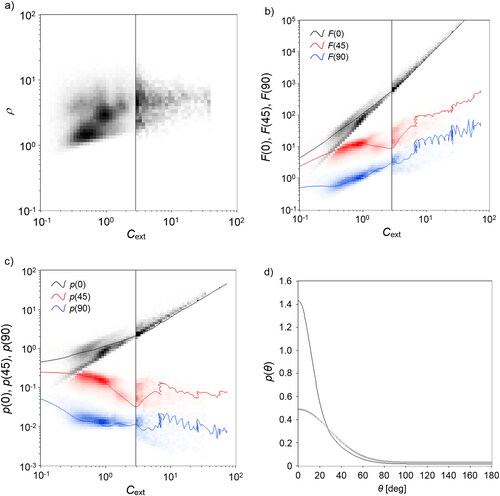
In Figure 4 we report experimental results obtained from early measurements in a relevant environment, the city of Milan. In this work, we report the whole data set as well as the basics of data analysis and interpretation described above. Discussing the temporal change in the optical properties of the particles, or characterizing them with independent measurements is beyond the scope of the present work. However, this could be an interesting subject for future studies. Solid lines in Figure 4b are still referred to water droplets, reported here as a guide to the eye for a better insight into the experimental data and in order to compare data to Figure 3b. Unlike the case of the water droplets in Figure 3, since now both the shape and composition of the particles are unknown we do not pursue an inversion by any model but limit ourselves to an analysis of the scattering data. Firstly, data show the presence of a population of particles generally smaller than in Figure 3 (roughly speaking, with smaller $C_{\mathit{ext}}$). Moreover, data exhibit a larger spread within the $(C_{\mathit{ext}},\mathrm{ }\rho )\mathrm{ }$ plane with respect to water droplets (panel a). This is attributable to non-spherical or/and non-compact structures (Villa et al. 2016; Potenza et al. 2017), as it is the case for aerosol of both natural and anthropogenic origin. Moreover, two populations can be easily distinguished, and therefore treated accordingly when interpreting data. In particular, the population in the upper left region of the $(C_{e\mathrm{x}t},\mathrm{ }\rho )$ plot cannot be explained as due to particles of any dielectric material with a reasonable refractive index, while it is fully compatible with particles composed by absorbing material (Mariani et al. 2017). Thanks to the single particle approach, we can also associate each event in the $(C_{\mathit{ext}},\mathrm{ }\rho )$ plot to the corresponding one in the $F$ plots. This shows that the same particle population corresponds to the events with the smallest $F\left(0\right)$ values for any given $C_{\mathit{ext}}.$ In the data set reported in Figure 4, the absorbing fraction amounts to approximately 25% of the total population in number concentration.

Figure 4. Results obtained in the city of Milan. Panels (a) (b) and (c) show data represented as in Figures 3a, b and c, respectively. Data on the right of the vertical line (C_ext>3) are multiplied by a factor of 10. Solid lines represent the Mie curves for water droplets for comparison. Notice the presence of two populations in (a). In (d) we show the phase functions fitted for the dielectric (solid line, black) and absorbing (circles, grey) portions of the population.

To recover the phase function, we can fit the expression in Equation (5)(5) $$p\left(\vartheta \right)=\mathit{Aexp}\left[-{\vartheta }^2/2{\sigma }^2\right]+\mathit{Bexp}\left[-\vartheta /b\right]+C$$(5) to experimental data. Unlike the case of water, here we cannot safely assume a given $\mathit{ssa}$ for each particle, which would likely be $\mathit{ssa}\mathrm{ }<\mathrm{ }1.$ We then rely on an estimate of typical $\mathit{ssa}$ values (Onasch et al. 2015). This is still enough information to feed the radiative transfer models, that need the optical properties averaged overall the considered population. Moreover, the single particle approach allows us to separate subsets of the population, associating each particle with the corresponding $C_{\mathit{ext}},$ giving an estimate for the average $\mathit{ssa}$ and evaluating average optical parameters for the chosen subset. Once the best fit for the phase function is found, we also calculate the asymmetry parameter, $g.$

For example, in recovering the optical properties from Figure 4, we can attribute effective values for the $\mathit{ssa}$ suitable for particles in different regions of the plot. Assuming an average $\mathit{ssa}\mathrm{ }=\mathrm{ }0.95$ for the dielectric particles the following parameters are obtained from the experimental data: $$p\left(0\right)=1.43, p\left(45\right)=0.135 \text{and} p\left(90\right)=0.016; 〈C_{\mathit{ext}}〉=1.38{\mu \mathrm{m}}^2, \text{and} \mathrm{g}=0.055$$ where ${⟨C}_{\mathit{ext}}⟩\mathrm{ }$ is averaged over the population. By imposing $\mathit{ssa}\mathrm{ }=\mathrm{ }0.8$ for the absorbing ones (Onasch et al. 2015), we have: $$p\left(0\right)=0.49,p\left(45\right)=0.173\text{and}p\left(90\right)=0.0295;〈C_{\mathit{ext}}〉=0.56{\mu \mathrm{m}}^2, \text{and} \mathrm{g}=0.043$$

Finally, assuming $\mathit{ssa}\mathrm{ }=\mathrm{ }0.65$ for the same population yields: $$p\left(0\right)=0.65,p\left(45\right)=0.230\text{and}p\left(90\right)=0.039;〈C_{\mathit{ext}}〉=0.56{\mu \mathrm{m}}^2, \text{and} \mathrm{g}=0.046$$

Notice that the average phase function is angularly more extended in the absorbing case than the previous one, accordingly to the fact that for any given $C_{\mathit{ext}}$ absorbing particles are smaller in size whereas their scattering lobe is larger. This is an example of how our approach can be adopted to give constraints to the entire scattering function. The phase functions recovered from the first two cases are represented in Figure 4b.

In order to test the impact of the aerosol optical properties on radiative transfer processes, we compare three cases obtained from data shown in Figure 4 by following three approaches for extracting the numerical parameters to feed the models:

1. by distinguishing the absorbing component from the dielectric one (Mix case). The case with $\mathit{ssa}\mathrm{ }=\mathrm{ }0.80$ for the absorbing particles has been considered here, while we assigned a value $\mathit{ssa}\mathrm{ }=\mathrm{ }0.95$ to the other population (see above). The average is $\mathit{ssa}\mathrm{ }=\mathrm{ }0.933,$ weighted on the optical depths, which is a common procedure.

2. by assuming one population with an effective $\mathit{ssa}\mathrm{ }=\mathrm{ }0.95$ (Die case)

3. by inverting the measured $C_{\mathit{ext}}$ values under the spherical particle assumption through Mie theory, by assuming a refractive index (Inv case).

We assume the same optical depth in all three cases. Therefore, the basic Lambert-Beer-Bouguer behavior providing the direct irradiance at ground (Edir) is unchanged. For small optical depths, Edir is the dominant contribution to the power balance. We then discuss the influence of the phase function and the presence of small, absorbing particles on the radiative transfer, thus elucidating the quantitative effect of distinguishing populations with different optical properties. In the first two cases (Mix, Die), we rely on our measurements to extract the optical properties as discussed above. In case 3) (Inv) we obliterate the knowledge of the phase function fitted to data and introduce the one calculated from the inversion. Accessing the entire set of optical properties from just one parameter is clearly limiting, but it quantitatively underlines the effect of changing the phase function and the strong limitation of assuming spherical particles. We are not interested in assessing the best choice of the refractive index: we will just show the discrepancies arising from the use of different methods to extract the optical properties from the same population of particles. We set a refractive index $n\mathrm{ }=\mathrm{ }1.5+0.01i.$ Mie theory provides the corresponding $C_{\mathit{ext}}$ values for a range of sizes, that allow to invert experimental data and to calculate the average phase function and the single scattering albedo value, $\mathit{ssa}\mathrm{ }=\mathrm{ }0.951.$

By using numerical simulations, we performed a sensitivity analysis by means of the consolidated LibRadTran software package and its Uvspec radiative transfer model (RTM, Mayer and Kylling 2005). Radiative transfer calculations are based on the extraterrestrial spectrum described in Kurucz, Barbuy, and Renzini (1992). Standard DISORT RTM solver is employed to perform monochromatic simulations at 635 nm (the laser wavelength). Finally, the Sun is considered 54 degrees above the horizon, or a solar Zenith angle of 36 degrees. Vertical concentration profiles are based on the OPAC software package (Hess, Koepke, and Schult 1998). We assumed a standard Optical Properties of Aerosol and Clouds (OPAC) height profile, continental polluted. By using the average $C_{\mathit{ext}}=1.17$ measured from our SPES data, we obtain the corresponding vertical number concentration profile. We adopted this concentration gradient as a reference to calculate the corresponding aerosol optical depth, defined as in Chandrasekar (1960) or Mayer and Kylling (2005). In view of our approach here, the chosen parameters might not describe precisely the atmosphere where we measured the dust optical properties. Along this line, we also consider the surface albedo to be negligible, to exclude multiple soil-atmosphere reflections and better evidence the effects of pure scattering from aerosols. The Mix case will be considered as the reference to which the other cases can be compared in terms of the sensitivity upon the parameters relevant for radiative transfer. Both the downward diffuse spectral irradiance at ground (Edn) and the upward diffuse irradiance at the top of the atmosphere (Eup) have been considered. For the sake of completeness, we also report the direct (Edir) and the global (Eglo) irradiances impinging onto the ground. Finally, by exploiting the power balance, we give an estimate of the fraction of the irradiance which is absorbed by the scattering centers (Eabs). The results are summarized in Table 1; spectral irradiance values are expressed in mWnm⁻¹m⁻².

Table 1. Numerical results obtained with the established LibRadTran software package and the UVspec RTM as described in the text, to compare the influence of different sets of optical parameters obtained from the data in Figure 4. Mix: two populations; Die: purely dielectric; Inv: Mie inversion. Spectral irradiance values are expressed in mWm⁻²nm⁻¹.

	Mix	Die	Inv	Die-Mix	Inv-Mix
Edir	909	909	909	0	0
Edn	203	207	238	4	35
Eglo	1112	1116	1147	4	35
Eup	84.4	86	58	1.6	−26.4
Eabs	63.6	58	55	−5.6	−8.6

Discrepancies between the Mix and Die case are limited to +2% for the Edn and −2% for the Eup. This shows that a precise knowledge of the different species, as achieved by SPES, allows to refine the optical parameters within an accuracy that is comparable to what needed for discussing the radiative balance of the Earth system (see Stocker et al. 2014). By contrast, the simpler interpretation based on spherical particles gives discrepancies up to about 30%, almost completely ascribed to the phase function. This is the reason why methods like the polar nephelometers are considered so important. Absorption is also interesting: differences are more relevant, larger than 5 mWnm⁻¹m⁻², with a relative difference up to 9% in the Mix-Die comparison. This results from the introduction of small absorbing particles, and shows that in the Mix case the power absorbed by the atmosphere is larger than in the Die case; by contrast, the latter provides a larger absorption at ground. This comparison shows that introducing a population of absorbing airborne particles appreciably affects the irradiation balance. The opportunity to distinguish different populations ultimately comes from the single particle measurement, which is definitely more effective in approaching aerosol optical characterization, as discussed in detail for example in (Sanford et al. 2008).

6. Conclusions

Experimental data show evidence of the importance of multiparametric characterization and the additional robustness of particle-by-particle approach. The instrument described here takes advantage from the SPES approach, thanks to the self-reference, self-calibrating method providing unique information for each measured particle. As already proven in the past (Potenza, Sanvito, and Pullia 2015; Mariani et al. 2017), statistical approaches applied to populations measured by single particle methods open completely new perspectives in interpreting the optical properties of airborne dust. Accessing the set of parameters needed to feed radiative transfer models is possible by introducing minimal assumptions, and an almost model independent phase function is recovered from experimental data. Preliminary tests performed by inserting the recovered optical properties into radiative transfer models show the importance of a precise measurement of the extinction cross section, accordingly to the current understanding of the Community. Moreover, experimental data have clearly shown that accessing one parameter only, such as either the $C_{\mathit{ext}}$ or $F\left(90\right)$ (as it is done in many single particle devices), leads to important errors in assessing the radiative transfer. The need of a simplified model for interpreting one-parameter experimental data unavoidably introduces inaccuracies coming from the actual heterogeneous and complex structure of the particles. Specifically, even an accurate measurement of the extinction cross section is not enough if data are not supported with any additional parameter, since different particle species with different optical properties for a given $C_{\mathit{ext}}$ coexist. This is evidenced in our data for the absorbing particles that, irrespectively of their nature and structure, clearly show important differences in radiative properties and phase functions that can be fitted to data. As shown here, our multiparametric data set is capable of setting constraints having relevant effects on the evaluation of light transmission and scattering in the atmosphere. The instrument has been tested and employed on the field, including under extreme conditions, and proved to be robust enough to be a good candidate for long term campaigns.

Acknowledgments

This article is a contribution to the PNRA16_00231 project “OPTAIR” (2017-2019). We thank the two anonymous Referees for their useful suggestions.