Development of an ultraviolet constant angle Mie scattering detector toward the determination of aerosol growth kinetics in the transition and free molecular regime

Abstract

The measurement of aerosol growth kinetics at ever smaller sizes toward the transition and free molecular regime is of interest to provide for validation of theoretical predictions. Such measurements remain challenging to accomplish, particularly those occurring in the kinetic regime. Toward this goal, an instrument based on the ultraviolet constant angle Mie scattering (UV-CAMS) method was developed. The instrument utilizes adiabatic expansion to cause supersaturation and drive aerosol growth. Aerosol particles growing by water condensation are illuminated with a pulsed UV laser at 337 nm wavelength and a reference laser with red light (wavelength of 632 nm). The scattered light fluxes at 30° are measured simultaneously and are then compared with size resolved Mie scattering calculations providing aerosol growth measurements. The growth curves obtained from UV match those from the red laser. These measurements allow us to see the first Mie peak for UV scattering for particles in the 500 nm range. This is an almost two-fold resolution increase compared to the smallest particles that can be seen via red laser scattering in similar conditions (first Mie peak above 900 nm).

Editor:

• Hans Moosmüller

Introduction

Aerosols are highly relevant for the environment and industry due to their impact in pollution, weather and global warming and also because their properties can be exploited for useful technologies. Understanding aerosol dynamics is essential to predict such properties, but aerosols spanning between molecular and macroscopic scales, and evolving in wide temporal ranges make the task difficult. This is the reason why our understanding of the initial stages of aerosol dynamics is still incomplete. In the environment many aerosols have long been given the reputation of pollutants to the environment. More recently, it has been shown that global warming, traditionally attributed to the presence of greenhouse gases (Cox et al. 2000), actually is greatly influenced by radiative forcing from aerosols. And this phenomenon causes the largest uncertainties in climate modeling (Liu and Daum 2002; Stocker et al. 2013). Furthermore, aerosols and clouds have been shown to be a sink for atmospheric trace gases with rates dependent on aerosol features (Kolb et al. 2010). With regard to industrial aerosols, it has been reported that many macroscopic properties of industrial relevance depend on the primary particle size and morphology defined in the initial stages of aerosol growth. (Neeleshwar et al. 2005; Nguyen and Flagan 1991; Vazquez-Pufleau 2016; Vazquez-Pufleau et al. 2020; Vazquez-Pufleau and Yamane 2020; Vazquez‐Pufleau 2019). Therefore, improving our understanding of the initial stages of aerosol growth can enhance our prediction capabilities for atmospheric phenomena and provide significant technological advances for industrial and medical (Diebolder et al. 2018) applications.

Aerosols span a wide range of sizes that can be divided into different domains or regimes and each of them is dominated by different transport processes. Obtaining an accurate prediction depends on understanding the regimes in aerosol evolution, and their dominant processes. The first step in aerosol formation is nucleation, in which a new phase, solid or liquid, emerges from the gas phase. After nucleation, the incipient nanoparticles grow in a kinetic dominated regime, denoted as free molecular regime. In this regime particles are smaller than the distance gas molecules need to travel to collide with each other in average (denoted as mean free path). The regime comprising aerosol nucleation and the initial stages of growth has not been completely elucidated (Bunker et al. 2012; Wu and Flagan 1987; Wu and Flagan 1988) in part because, of the hurdles imposed by its intrinsic fast dynamics and small scale. This is despite the apparent simplicity of nucleation from a theoretical point of view where the low amount of molecules in consideration makes it a rare process statistically speaking. On the other end of the size scale, for particles much larger than the mean free path of the gas, the continuum regime dominates (Friedlander 2000), a regime governed by thermal conductivity and diffusivity (Winkler et al. 2004). For particles in the size range comparable to the mean free path both kinetic and continuum effects play a role which is why this regime is the so-called transition regime. Aerosol dynamics in this regime is the hardest to quantify from a fundamental point of view.

The measurement of aerosol dynamics demands instruments with sufficient temporal and spatial resolution to capture such small and fast processes. A detailed discussion of available instruments and techniques for characterizing aerosols can be found under (McMurry 2000), (Moosmüller, Chakrabarty, and Arnott 2009) and (Kolb et al. 2010). The vast majority of commercial aerosol characterization instruments provides a snapshot of the aerosol properties, especially number concentration and size. However, little information is obtained on aerosol growth kinetics beyond the instrumental intrinsic sampling rate, which is typically one second at best. In order to understand the mechanism of numerous atmospheric and industrially relevant aerosol growth processes, it is necessary to utilize an instrument capable of measuring much faster, with sub-ms resolution, in a well-controlled system, without disturbing it, and preferably in situ. Such features are available in aerosol instrumentation based on optical detection including those described by Mie scattering (Horvath 2009; Nagy et al. 2007; Szymanski, Nagy, and Czitrovszky 2009; Szymanski et al. 2002; Winkler et al. 2008).

Several researchers have developed instruments to measure heterogeneous nucleation, focusing at different conditions and materials of interest. Pioneers include the work of (Sutugin and Fuchs 1968; 1970) Reports exist on the usage of the constant angle Mie scattering (CAMS) method based on a fast expansion and recompression pulsed chamber to separate homogeneous nucleation from subsequent growth. In the experiment a He-Ne laser (λ = 632.8 nm) at 15° was utilized for water (Fladerer and Strey 2003) and cryogenic gases (Fladerer and Strey 2006; Iland et al. 2009; Iland et al. 2007). The system water in air using a HeNe red laser (λ = 632 nm) provided aerosol growth measurements in the continuum regime (Wagner 1985; Winkler et al. 2004). Growth due to water and n-propanol in air was also measured at several different angles simultaneously using a blue laser (λ = 488 nm) (Pinterich et al. 2016). Also, an expansion pulsed wave tube setup with an argon ion laser (λ = 488 nm) and a photomultiplier at 90° from the incoming laser has been reported. Such instrument was used to measure particle growth in the transition and continuum regime for binary and ternary mixtures of water, n-nonane and methane at high pressure (Peeters, Hrubý, et al. 2001), as well as n-pentanol in helium (Peeters, Luijten, et al. 2001). Further experimental developments and a theoretical overview in homogeneous nucleation can be found elsewhere (Wyslouzil and Wölk 2016). In the current study, we have utilized a narrower wavelength and a smaller angle because the Mie scattering ripples are better resolved in the forward direction than in the backward direction.(O Preining et al. 1981; Szymanski, Nagy, and Czitrovszky 2009).

Mie theory combined with experiments can be used to determine growth rate of monodisperse aerosols. The theory provides the relationship between scattering intensity and particle diameter for a given wavelength and the experimental measurement provides temporally resolved scattering intensity. Mie scattering is a specific solution to Maxwell´s equation of electrodynamics. Calculations are generally difficult to solve by hand (Wiscombe 1980), but now, thanks to computers, Mie theory online libraries (pre-built codes) can be routinely used to calculate Mie scattering patterns (Craig, Bohren, and Huffman 1983), or to calculate the complex refractive indexes of individual aerosols (Sumlin, Heinson, and Chakrabarty 2018). Mie theory predicts scattered intensity to be a function of the size parameter (α). This theory is applicable to spherical objects of any size but requires tedious calculations that converge more slowly for increasing size parameter α, which is proportional to the ratio of diameter (d_p) over wavelength (λ), in such a way, that α = (πd_p)/λ. This expression shows that for a fixed wavelength of the used laser light, the size parameter is directly proportional to the droplet size. Similarly, for the same size parameter, the diameter required to obtain similar scattering intensity can be lowered by using shorter wavelengths. Therefore, utilizing UV light allows for measuring aerosol growth rate at smaller sizes. An approach that to the best of our knowledge has not been explored in the past.

The constant angle Mie scattering (CAMS) method is a powerful and accurate method to determine aerosol growth rate and number concentration. It was developed to measure absolute total number concentration and particle growth rate of monodisperse aerosols with sub-ms resolution (Wagner 1985). This method requires knowledge on the refractive index of the used material, which depends on the wavelength of the incoming light. The refractive index of water is available in the literature in tabular form (Segelstein 1981). The CAMS measurement is based on the simultaneous noninvasive and highly time resolved detection of extinction and scattered light of a given wavelength at a constant angle (Szymanski and Wagner 1990). Scattered light intensity is several orders of magnitude lower than the incoming light, but its measurement can be achieved with a photomultiplier (Pinnick, Rosen, and Hofmann 1973). For aerosols growing monodisperse, total observed scattered light is an incoherent superposition of the light scattered by all individual droplets. Therefore, the intensities and not the amplitudes are added and no interference is observed (Wagner 1985). Scattering intensity starts from a value close to zero and increases as the diameter gets larger until reaching the first Mie maximum, which is then followed by a minimum and then by a new maximum and so on, forming what appears as global extrema. Superimposed on this coarse structure, fine structured ripples can also be observed. The global extrema observed correspond to a diffraction pattern from the growing droplets, while the ripples result from resonance phenomena within the droplets. Such scattered light curves are measured experimentally as a function of time. By comparing both, experimentally measured and calculated Mie scattering curves, growth curves can be obtained. A discussion on the CAMS method can be found in the supplementary section. A schematic of the cycle, its principles and the scattering signal produced can be seen in Figure S1.

In this work, the CAMS methodology is tested using UV radiation in order to detect smaller particles with ms time resolution. Measuring small particles with high temporal resolution is important because the mass and thermal accommodation coefficients can only be measured in the kinetic regime. In the continuum regime such coefficients are not retrievable because the diffusion and thermal conductivity of the gas dominate the process. Direct measurement of accommodation coefficients may become feasible if the shortest possible wavelength is applied. One of the limits of utilizing Mie scattering for measuring aerosol growth rate with the CAMS method is determined by the wavelength at which the carrier gas starts absorbing the radiation. This limit is around 60 nm for helium (Sando and Dalgarno 1971), ∼87 nm for argon, ∼145 nm for nitrogen (Wilkinson 1957) and ∼180 nm for oxygen (air) but this value increases above 220 nm if ozone is formed (Tanaka, Inn, and Watanabe 1953). The difficulty of going beyond this limit is that the absorption slope is almost a step function for pressure near atmosphere, where a jump from 0 absorption to almost 100% is achieved within few centimeters for a modification of only a few nm in the wavelength. Additional factors are relevant for determining the intensity of gas absorption in these regions, including pressure, transmission thickness and initial intensity. The present study is a step toward this direction. By venturing with UV light and pulsed lasers we tackle some of the challenges that need to be addressed to achieve such goals. Challenges addressed here include the development of a setup and process that has enough stability and reproducibility to provide thousands of consistent growth rate measurements, and the successful usage of a UV pulsed laser with a wavelength of 337 nm to reconstruct aerosol growth curves. The results of single pulses were integrated over several thousands of measurements and self-programmed python code was used for reconstructing time resolved Mie scattering curves from single pulses. Such curves were then converted into aerosol size evolution plots as a function of time by comparing them with theoretical Mie scattering curves. The UV laser growth curves show consistency with the red laser growth curves.

Materials and methods

The instrumental setup contains several subsystems. Different aspects of the instrument are illustrated graphically. Figure 1 is a schematic of the UV-SANC including peripheral equipment. Figure 2 is a schematic of the UV SANC expansion chamber and sensors layout. The drawings and dimensions of the expansion chamber can be found in Figure S2. The transient temperature profile due to conduction inside the chamber is shown in Figure S3. For simplicity, the description of the components of the UV SANC is divided into three sub-sections involving the aerosol seed generation, the UV-SANC instrument and the electronics and optics.

Figure 1. Schematic of the UV CAMS instrument including peripheral process controllers, sensors, detectors and ancillary equipment.

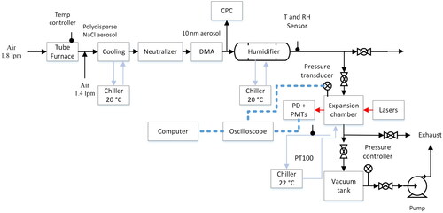
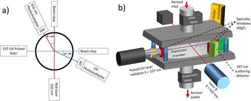
Figure 2. (a) 2 D Schematic (top view) of the Dual wavelength UV CAMS. It primarily consists of two lasers, a red one (632 nm) and another in the UV (337 nm) as well as its respective photomultipliers to detect the scattering signal. Each of the branches also has a lowpass filter (LPF) or highpass filter (HPF) to ensure that the UV detector does not receive light from the red laser and viceversa. (b) Schematic illustrating the 3 D arrangement of lasers and detectors with respect to the expansion chamber aerosol inlet and outlet.

Monodisperse aerosol generation

Figure 1 shows a diagram of the experimental setup. It starts with compressed air, produced by an air compressor (SF4, Atlas Copco, Belgium), dried by a membrane dryer (SD-4N-7, Atlas Copco, Belgium). Oil residuals and particles were removed with high efficiency coalescing filters (PD10+ and DD10+ Atlas Copco, Belgium). A HEPA filter (HEPA Capsule, Pall, USA) was used before the connection to our setup to remove any particles from the gas supply. A pressure regulator (Excelon, Norgren, UK) was used to keep the inlet pressure constant at 1.1 bar. Then, the gas flowed through needle valves (DK Lok, USA) and the flow rate was monitored through rotameters. A 1.8 lpm flow passed through a quartz tube containing a quartz spoon filled with sodium chloride (NaCl >99% Sigma Aldrich ACS, Switzerland). The tube and spoon were heated by a tubular furnace (ROR 1,8/18,5, Heraeus, Germany) which at appropriate temperature settings evaporates some of the salt and forms nanometer sized aerosols. The furnace is controlled by an RS controller (ESM4430, EMKO, Turkey) and powered by a high current power supply (QPX1200SP, TTi, USA). After the furnace, a homemade quartz tubing with 4 radial gas inlets receives 1.4 lpm of air and is used to dilute the aerosol flow and quench its dynamics so that the mean of the size distribution remains around 10 nm size range. Then aerosols pass through a concentric cooling device made of quartz and with an external water cooling jacket. The working fluid for the heat exchange in this cooling jacket was recirculated and controlled at a temperature of 20 °C by a Lauda chiller (RM6 Lauda, Austria). The aerosol stream was then passed into a radioactive neutralizer (Am²⁴¹, Tapcon Analysis Systems, Austria) and then through a nano differential mobility analyzer (DMA, Tapcon Analysis Systems, Austria), which was supplied with a high voltage of 620 V from a high voltage power supply. (Leybold P15VA, Germany) and was monitored with a (Fluke 73 III Multimeter, USA). The sheath flow of 21 lpm for the DMA was supplied by a recirculating flow unit (FCU-10 Tapcon Analysis Systems, Austria) which cleaned the flow by means of activated carbon, a HEPA filter and silica gel. At these conditions, a monodisperse aerosol of 10 nm is selected. After the DMA, the flow was diverted in two streams. The first stream consisted of 1.5 lpm and was fed into a condensation particle counter (CPC Model 3776, TSI, USA) to monitor the number concentration of the aerosols. The second stream carried the remaining flow toward the UV-SANC setup.

Ultraviolet size analyzing nuclei counter (UV- SANC) setup description

The stream entering the UV SANC device was passed through a homemade humidifier consisting of two concentric stainless steel cylinders welded together, with the aerosol flowing in the inner tube and cooling liquid flowing in the outer cylinder. To humidify the flow, a single layer of absorbent filter paper was rolled and introduced in the humidifier and was flooded with ultra-high purity water (water HPLC Plus sigma Aldrich, Switzerland). The temperature control for the humidifier was provided by a chiller (Lauda RM6 Lauda, Austria) with set point at 20.0 °C. After the humidifier, the flow temperature (T) and relative humidity (RH) were measured by a T and RH sensor (SHT75, Sensirion, Switzerland) and recorded by a Raspberry Pi. (Model B, Raspberry Pi 3, UK). The flow then entered the solenoid valve array of the expansion chamber which was cycled and controlled by a second Raspberry Pi. The Raspberrys and the computer were connected through an intranet network switch (DES-105, D-Link, China) for data acquisition and cycle synchronization. The cycle lasted one minute to guarantee the presence of fresh aerosol in the chamber for each experiment which upon completion was immediately restarted. During each cycle, the flow could either go into the chamber by means of an actuated ball valve (compact power, RUB, Italy), or through a solenoid valve (Model82641009151, Buschjost, Germany) into the exhaust. This valve type was also used to control the pressure in the vacuum tank and downstream of the chamber for flushing it. The expansion chamber consisted of an aluminum AlMgSi₁ cylinder machined and professionally anodized to optical degree to minimize reflections. Selected chamber drawings are shown in Figure S2. Calculations of heat transfer in the interior of the chamber based on air conduction can be found in Figure S3. They show that even for expansions with twice pressure drop as the maximum used in this study, heat transfer due to conduction would need more than 300 ms to start producing a measurable increase in the temperature at half the chamber radius. Therefore, it is considered that heat conduction does not influence growth dynamics for the first 300 ms after the adiabatic expansion. On the top of the expansion chamber, fresh aerosols enter via the actuated ball valve. On the bottom, a solenoid valve (valve model 8570500.8401, Buschjost, Germany) produces the adiabatic expansion. The expansion chamber is water cooled and its temperature is controlled and monitored with a chiller set at 22.00 °C (Lauda variocool VC1200, Lauda, Austria). Also, the temperature of the chamber is indirectly monitored by measuring the temperature of the cooling fluid at the outlet of the chamber jacket with a PT100 sensor (WT330-E3, LEMO, Switzerland). The temperature is monitored by an Omega platinum series monitor (CS8DPT Omega Engineering Inc., USA). After the expansion chamber there is a 10 liter stainless steel cylinder (CRVZS-10, FESTO, Germany) operating as a vacuum tank. It is connected to the vacuum side of a pump. The pressure in the vacuum tank is measured by a pressure transducer (PX309, Omega Engineering Inc., USA) and controlled by a pressure controller and monitor (CN7833 Omega Engineering Inc., USA), which combined with a manual needle valve provide normally +/−1 mbar control of the pressure set point. To ensure constant flow through the UV CAMS instrument and stability to integrate over several thousands of cycles, all outlets are connected to a homemade critical orifice with a nominal flow of 1.42 lpm. After the pump, the exhaust flow passes through a HEPA filter before being released into the atmosphere. All flows were validated with a standard air flow calibrator (Gilibrator, Sensidyne, USA).

Electronics and optics of the expansion chamber

The lasers and photodetectors are connected to the chamber by means of six windows as schematically displayed in Figure 2. For the ports relevant for the red laser, three borosilicate glass windows (5 mm Borofl part no 43888, Edmund Optics LTD, UK) were used. The other three windows used for the UV branch are made of magnesium fluoride (5 mm MgF₂ windows part No 64092, Edmund Optics LTD, UK). A red laser (632 nm He Ne, uniphase model 1135, USA) is used as a reference operated by a power supply (Model 35974, Melles Griot, USA). A photomultiplier (H7827-002, Hamamatsu, Japan) is used for detecting scattered light and is located under an angle of 30° in forward direction from the light source. Between the chamber and the detector, a light filter (TS Long pass filter 400 nm Part no 49024, Edmund Optics Ltd, UK) removes the UV light so that the detector intended for the red laser does not receive the backward Mie scattering caused by the UV laser. A horizontally adjustable slit (VA100C/M Thorlabs, USA) limits the amount of light that can physically reach the detector. The photomultiplier is connected to a power supply (IPS 4304, RS PRO, UK), which also allows for tuning the gain for optimizing the signal to the oscilloscope measurement range. The second detector branch (UV) receives its light from a UV 4 ns 30 Hz pulsed Laser 337 nm N₂ (VSL 337 ND-S, Thermo Laser Science, USA). The detector side is the same than for the red branch except that in this case a low pass filter (Short pass filter UV 550 nm part number 49160, Edmund Optics Ltd, UK) is used to avoid the red light from reaching the UV photomultiplier. The pressure drop after each expansion is measured by a pressure transducer (Kistler 7261, Kistler, Switzerland) and a pressure recorder (Kistler Charge Meter Type 5015, Kistler, Switzerland) which provides a real time signal measurable in V for the pressure in the chamber. This signal and also the two signals from the photomultipliers are recorded with an oscilloscope (Picoscope 2000 Series2406B, Pico Technology, UK) in a picoScope data file (.psdata) which can then be converted into a text file and be processed with both open source and self-programmed python code.

Results and discussion

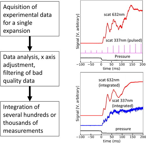
The UV laser utilized provided pulsed and not continuous light. Therefore, it was necessary to measure the same experimental condition several hundreds and in some cases even thousands of times in order to obtain sufficient data to reconstruct a time resolved scattering curve from the few UV data points obtained after each expansion. Figure 3 shows a schematic of the process utilized to reconstruct time resolved Mie scattering curves from pulsed measurements. For each measurement, the acquisition of signal before the expansion is also required to establish the background level. Measurements for each supersaturation degree were acquired for between 700 to 2500 times. Then, the x axis of the plots was adjusted so that the red scattering signal would always start at the same plotted time, and the pressure drop would be located at time 0. Measurements not fulfilling minimum quality requirements (typically less than 5%) were not considered further. The filtered data was then integrated producing coherent peaks for the UV laser that could then be quantified. The red laser scattering signal was also subjected to integration for quality control and a reduction of the sharpness of the ripple structure was observed. Such smoothing is expected due to small variations in the scattering signal over several hundreds of cycles. But does not prevent correct identification of the major peaks. The data from Figure 3 correspond to a super saturation (S) of 1.25.

Figure 3. Flow diagram of data acquisition for a single expansion, and the result after integration of several hundreds to thousands of measurements. The integration process utilizes data quality tools and x axis adjustment to ensure all scattering lies within tight limits. Nevertheless, due to minor variabilities of the process, it is visible that the red scattering signal degrades slightly after integration. However, this process permits reconstructing the scattering signal from the UV source, which would otherwise be impossible from a pulsed laser.

The reason behind using a red laser in addition to the UV laser is that the well-known experimental Mie ripple structure from a 632 nm is a necessary reference to validate the UV maxima count and avoid mis-assignment between experiment and theory. Mie theory does predict that narrower wavelengths allow detection of smaller particles. However, this also causes a reduction in the scattering intensity as a function of wavelength square (O Preining et al. 1981) and is affected by the change in refractive index as a function of wavelength (Segelstein 1981). Such system attribute makes the global extrema and ripple pattern recognition increasingly difficult with decreasing wavelength. If the peaks in the signal lie near the noise level, growth analysis is no longer trivial. For this reason, a second laser of a visible wavelength is used at 632 nm so that the first Mie scattering pattern of the red laser can be uniquely identified. This can be used as a reference to match the corresponding Mie peaks from the UV because there is a region where both scattering patterns provide measurements at coincidental time and particle size, allowing for temporal and size matching from the two curves of different wavelengths. In addition, any unexpected effect on the growth curve induced by the UV laser could be easily observed as a modification in the red laser growth curve. For these reasons, the aerosol growth curve determinations were performed using a dual wavelength CAMS with coherent lasers at two different wavelengths.

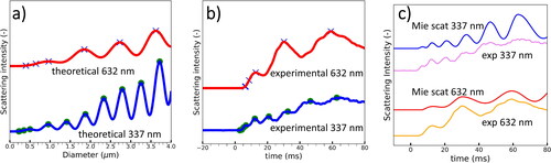
The growth curves are obtained by comparing the theoretical Mie scattering curves with the experimental Mie scattering curves. Theoretical Mie scattering curves are computed using the python programing language by means of the open source scatterlib library. The accuracy of the library and the used code were validated by comparing its results with theoretical growth curves based on Mie scattering reported in the literature (Szymanski and Wagner 1990). In order to obtain experimental growth curves, it is necessary to compare the position of recognizable patterns in the theoretical (Figure 4a) and experimental scattering curves (Figure 4b). The relationship between diameter and time is a non-linear function. A program was coded in order to identify the local maxima and a filtering function was used to smooth both the theoretical and the experimental curves. This was necessary to ensure correspondence of the theoretical features to the resolution of the measured and integrated peaks. Then, the correspondence between the peaks from the temporally resolved experimental scattering signal could be assigned to a specific particle size. After matching the peaks, the intervals between the peaks were calculated linearly for simplicity and for displaying the correspondence of theory and experiment in Figure 4c). However, it should be noted that the only experimental values further used for the growth curves correspond to the identifiable peaks of the scattering signal. For the first Mie maximum also the point corresponding to half of the maximum is reported. X axis conversion from time to diameter was executed for red and UV signals independently.

Figure 4. (a) Theoretical Mie scattering curves calculated based on python library scatterlib. (b) Experimental Mie scattering curves measured with the UV CAMS that correspond to a pressure drop of 100 mbar (S = 1.25). The maxima are found using a simple algorithm that identifies local maxima. (c) By using a nonlinear x axis maxima matching of a) and b), a relationship between the diameter and time can be found and the theoretical growth curve can be plotted using the same axis than the experimental curve.

Growth curves for six different super saturations could be obtained following the procedure described above (Figure 5). Aerosol size evolution as a function of time from the UV signal is represented by circles while the crosses represent the same information obtained from the red laser. Information from both wavelengths match nicely in the overlapping region. In order to perform a growth rate estimation, the following assumptions were made and are justified as follows: The thermal effects of the enthalpy of condensation of water on increasing the temperature of aerosols have been found to be negligible (Winkler et al. 2004). Preliminary calculations on the thermal effects (Filippov and Rosner 2000) caused by radiation absorption indicate that small particles would heat up more rapidly upon absorbing photons, but at the same time are subject to more rapid cooling as they diffuse more rapidly. On the other hand, bigger particles have a lower surface to volume ratio and cool more slowly, but they also heat up more slowly upon absorbing a photon due to their increased mass. In both cases, the cooling effect through gas collisions is larger than any heating effect from photon absorption even for a 4 ns pulse such as the one produced by the UV laser. In any case, water is not expected to absorb the wavelengths used (632 and 337 nm) (Segelstein 1981). The effect of scattering from the NaCl seeds can be disregarded due to their negligible cross section, their small size and low concentrations. The carrier gas (air) is also not causing scattering at the wavelengths used (Tanaka, Inn, and Watanabe 1953). Loses through the MgF₂ windows that separate the expansion chamber from the lasers and detectors are negligible. Backscattering from the second wavelength is also negligible as a low-pass and a high-pass filter remove backscatter from the laser not intended to be measured by the photomultipliers. The Kelvin and Raoult effects can be neglected because the 10 nm NaCl seed utilized has a negligible contribution for both phenomena at the smallest measurable size (∼350 nm). Similarly, the impact of the NaCl seed in modifying the refractive index of the droplets is also negligible (Tan and Huang 2015) and was not included in the calculations.

Figure 5. Summary of the evolution of diameter for different supersaturations. Crosses are the values obtained from analyzing the 337 UV signal. Circles correspond to the 632 nm red laser measurement. The continuous lines are calculated based on theoretical size evolution calculations.(Vesala et al. 1997).

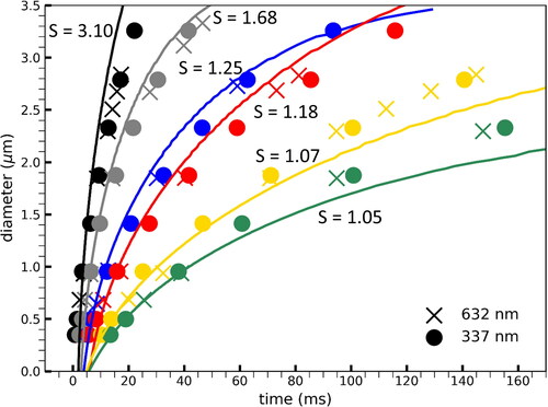
Taking into consideration the above discussed assumptions, an aerosol growth rate calculation was executed based on the condensation models from (Vesala et al. 1997) as a reference for the experimental data and also to observe the agreement between data produced by this new developed SANC and its predecessor (Wagner 1985). The parameters used for the theoretical calculations are the following: experimental values as measured by the system controllers and monitors, numerical solution using the Clement theory (Clement 1985), solution with a transitional correction theory that goes from continuum to free molecular regime from Dahneke (Dahneke 1983). Typically, it is assumed that the continuum regime occurs for Knudsen numbers (Kn) 0 < Kn < 10⁻³, slip flow between 10⁻³ < Kn < 10⁻¹, transition regime between 10⁻¹ < Kn< 10¹ and finally the free molecular regime between 10¹ < Kn and < ∞.(Darabi et al. 2012; Sundaram, Yang, and Zarko 2015) The Knudsen numbers (Kn) for both experimental wavelengths are reported in Table 1. The mass and thermal accommodation coefficients were set to one and the thermal diffusion factor was set to zero. The theoretical curves nicely replicate the experimentally observed trend and clearly follow the expectation that growth proceeds faster at higher saturation ratios.

Table 1. Knudsen number of particles detectable by the red and UV lasers scattering at 30° and a final pressure of 900 mbar.

Wavelength	Kn for first Mie peak	Kn half of first Mie peak
632 nm (red)	0.12	0.16
337 nm (UV)	0.22	0.32

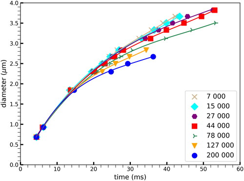
The effect of the number concentration on aerosol growth rate curves was tested in the UV SANC in the concentration range between 7000 and 200000 #/cm³. The results are presented in Figure 6. Vapor depletion during the initial stages of aerosol growth up to about 1000 nm droplet diameter is practically negligible. However, at later stages of aerosol growth, for conditions with high number concentration, the amount of water vapor available gets depleted more rapidly, slowing down the growth process. On the other hand, in the case of lower number concentrations, the aerosols can continue growing to larger sizes before water vapor gets depleted. These results are in good agreement with previous measurements using the CAMS method (Wagner 1975).

Figure 6. Effect of number concentration on droplet growth for a supersaturation of S = 1.68: at higher number concentrations the growth of the droplet size plateaus earlier than at lower number concentrations due to water vapor depletion.

An important challenge for the CAMS method is the low amount of scattered signal compared to the original light intensity. The scattered intensity with an angular resolution better than 1° is only a fraction in the order of 10⁻⁶ of the incoming intensity. Therefore, in the region where gases absorb heavily (mainly in the vacuum ultraviolet for inert gases), it is not easy to obtain any signal at all unless a very high light intensity is utilized. High intensity VUV sources are generally difficult to obtain and are prone to cause additional difficulties in the measurement such as temperature increase in the gas and potential re-evaporation of the particles, etc. In any case we encourage future researchers to attempt approaching such limits to determine kinetics of aerosol growth rate in the free molecular regime at atmospheric relevant conditions.” The results obtained in this work serve as a proof of principle that it is feasible to experimentally measure smaller sizes of aerosols with UV radiation. Growing droplets are formed in an expansion chamber which produces reproducible adiabatic expansions and process variables are well controlled and monitored. The whole system operates reliably, yet some improvements are also possible and will be addressed in future work.

Conclusion

In this work, a UV CAMS detector was designed, constructed and operated to measure aerosol growth curves in situ at sizes below those reported in the literature for this method in forward scattering. The instrument utilized a pulsed UV laser at 337 nm and a red 632 nm continuous wave laser as a reference. The measurements were carried out in the transition regime, at near atmospheric pressure and with Kn numbers as low as 0.32. The carrier gas used was air, which displays sufficient transmission at both wavelengths.

In this work, signal integration was utilized to reconstruct temporally resolved Mie scattering growth curves by utilizing a well-controlled setup with sufficiently reproducible and stable process variables and a suitable data analysis and processing code. The reproducibility of the cycle in the UV CAMS was sufficient to allow integration of measurements obtained through several thousands of expansion cycles for reconstructing the temporally resolved Mie scattering growth curves from a 30 Hz pulsed UV laser. This validates the feasibility of using the SANC to extract aerosol kinetics by using pulsed light sources such as the ones available at some free electron lasers (FEL), synchrotrons, and high power UV lasers.

The Mie scattering growth curve measured by a detector at 30° from the 337 nm light source produced a first peak at 500 nm, with half of the first peak height at 349 nm. This compares with the ones produced by a 632 nm red laser which are 934 nm and 684 nm for the first peak and half of its height, respectively. In addition, there is a remarkable agreement in growth in the overlapping region of the two laser signals. The growth in the chamber behaves as expected: particle growth is faster with higher super saturation (S). Particle growth also terminates earlier with higher concentration but this does not affect growth in the sub 1000 nm region.

The results obtained in this study pave the road toward the development of the vacuum ultraviolet size analyzing nuclei counter (VUV-SANC). Such an instrument could provide direct evidence on the mass and thermal accommodation coefficients in the free molecular and transition regime. Both coefficients are still under debate, and can only be measured in aerosol growth conditions dominated by the kinetic regime. Furthermore, such endeavors can help us to get closer in understanding nucleation. For achieving the required accuracy, the availability of a high power, high quality and accessible light sources in the vacuum ultraviolet is essential. A continuous light-source is ideal for this experiment but pulsed sources can also be used as shown in this study. However, for using pulsed sources in the reconstruction of growth curves, it is paramount to count with a fine tuned process control and a highly reproducible system.

Additional information

Competing financial interest: M.V.P., P. M. W. declare no competing financial interests.

Acknowledgments

We would like to thank Prof. Paul Wagner for his insightful advice and recommendations for the realization of this work, Christian Tauber for his SANC know-how and support, Paulus Bauer, Sophia Brilke, Dominik Stolzenburg, Harald Schuh and Peter Dangl for their help with technical matters, insightful discussions and support, and Steve McClain for useful discussions in optics. Also special thanks to Prof. Arndt and his group for lending us the UV pulsed laser. This work was supported by the ERC consolidator grant project under the FP7 excellence program “Ideas”, project No. 616075. We are also thankful to Marcello Coreno, Emiliano Principi and Heinz Amenitsch for useful synchrotron, instrumentation, and detection discussions, to Angelo Giglia, Konstantin Koshmak, and Stefano Nannarone for relevant beamline and data acquisition support. The research leading to this result has been supported by the project CALIPSOplus under Grant Agreement 730872 from the EU Framework Programme for Research and Innovation HORIZON 2020.

References

- Bunker, K. W., S. China, C. Mazzoleni, A. Kostinski, and W. Cantrell. 2012. Measurements of ice nucleation by mineral dusts in the contact mode. Atmos. Chem. Phys. Discuss. 12 (8):20291–309. doi:https://doi.org/10.5194/acpd-12-20291-2012.
- Clement, C. (1815/1985). Aerosol formation from heat and mass transfer in vapour–gas mixtures. Proc. R. Soc. London. A. Math. Phys. Sci. 398, 307–39. doi:https://doi.org/10.1098/rspa.1985.0037.
- Cox, P. M., R. A. Betts, C. D. Jones, S. A. Spall, and I. J. Totterdell. 2000. Acceleration of global warming due to carbon-cycle feedbacks in a coupled climate model. Nature 408 (6809):184–7. doi:https://doi.org/10.1038/35041539.
- Craig, F. B., F. Bohren, and D. Huffman. 1983. Absorption and scattering of light by small particles.
- Dahneke, B. 1983. Simple kinetic theory of Brownian diffusion in vapors and aerosols, in Theory of dispersed multiphase flow. The Mathematics Research Center, the University of Wisconsin–Madison: Academic Press, 97–133.
- Darabi, H., A. Ettehad, F. Javadpour, and K. Sepehrnoori. 2012. Gas flow in ultra-tight shale strata. J. Fluid Mech. 710:641–58. doi:https://doi.org/10.1017/jfm.2012.424.
- Diebolder, P., M. Vazquez-Pufleau, N. Bandara, C. Mpoy, R. Raliya, E. Thimsen, P. Biswas, and B. E. Rogers. 2018. Aerosol-synthesized siliceous nanoparticles: impact of morphology and functionalization on biodistribution. Int. J. Nanomed. 13:7375–93. doi:https://doi.org/10.2147/IJN.S177350.
- Filippov, A., and D. Rosner. 2000. Energy transfer between an aerosol particle and gas at high temperature ratios in the Knudsen transition regime. Int. J. Heat Mass Transfer 43 (1):127–38. doi:https://doi.org/10.1016/S0017-9310(99)00113-1.
- Fladerer, A., and R. Strey. 2003. Growth of homogeneously nucleated water droplets: a quantitative comparison of experiment and theory. Atmos. Res. 65 (3-4):161–87. doi:https://doi.org/10.1016/S0169-8095(02)00148-5.
- Fladerer, A., and R. Strey. 2006. Homogeneous nucleation and droplet growth in supersaturated argon vapor: The cryogenic nucleation pulse chamber. J. Chem. Phys. 124 (16):164710. doi:https://doi.org/10.1063/1.2186327.
- Friedlander, S. K. 2000. Smoke, dust, and haze. New York: Oxford University Press.
- Horvath, H. 2009. Gustav Mie and the scattering and absorption of light by particles: Historic developments and basics. J. Quant. Spectrosc. Radiat. Transfer 110 (11):787–99. doi:https://doi.org/10.1016/j.jqsrt.2009.02.022.
- Iland, K., J. Wedekind, J. Wölk, and R. Strey. 2009. Homogeneous nucleation of nitrogen. J. Chem. Phys. 130 (11):114508. doi:https://doi.org/10.1063/1.3078246.
- Iland, K., J. Wölk, R. Strey, and D. Kashchiev. 2007. Argon nucleation in a cryogenic nucleation pulse chamber. J. Chem. Phys. 127 (15):154506. doi:https://doi.org/10.1063/1.2764486.
- Kolb, C. E., R. A. Cox, J. P. D. Abbatt, M. Ammann, E. J. Davis, D. J. Donaldson, B. C. Garrett, C. George, P. T. Griffiths, D. R. Hanson, et al. 2010. An overview of current issues in the uptake of atmospheric trace gases by aerosols and clouds. Atmos. Chem. Phys. 10 (21):10561–605. doi:https://doi.org/10.5194/acp-10-10561-2010.
- Liu, Y., and P. H. Daum. 2002. Indirect warming effect from dispersion forcing. Nature 419 (6907):580–1. doi:https://doi.org/10.1038/419580a.
- McMurry, P. H. 2000. A review of atmospheric aerosol measurements. Atmos. Environ. 34 (12-14):1959–99. doi:https://doi.org/10.1016/S1352-2310(99)00455-0.
- Moosmüller, H., R. Chakrabarty, and W. Arnott. 2009. Aerosol light absorption and its measurement: A review. J. Quant. Spectrosc. Radiat. Transfer 110 (11):844–78. doi:https://doi.org/10.1016/j.jqsrt.2009.02.035.
- Nagy, A., W. Szymanski, P. Gal, A. Golczewski, and A. Czitrovszky. 2007. Numerical and experimental study of the performance of the dual wavelength optical particle spectrometer (DWOPS). J. Aerosol. Sci. 38 (4):467–78. doi:https://doi.org/10.1016/j.jaerosci.2007.02.005.
- Neeleshwar, S., C. L. Chen, C. B. Tsai, Y. Y. Chen, C. C. Chen, S. G. Shyu, and M. S. Seehra. 2005. Size-dependent properties of CdSe quantum dots. Phys. Rev. B 71 (20):201307(R). doi:https://doi.org/10.1103/PhysRevB.71.201307.
- Nguyen, H. V., and R. C. Flagan. 1991. Particle formation and growth in single-stage aerosol reactors. Langmuir 7 (8):1807–14. doi:https://doi.org/10.1021/la00056a038.
- O Preining, P., E. Wagner, F. G. Pohl, and W. Szymanski. 1981. Aerosol Research Part III Heterogeneous nucleation and droplet growth. Vienna, Austria: Institut für Experimentalphysik der Universität Wien.
- Peeters, P., J. Hrubý, and M. E. H. van Dongen. 2001. High pressure nucleation experiments in binary and ternary mixtures. J. Phys. Chem. B 105 (47):11763–71. doi:https://doi.org/10.1021/jp011670+.
- Peeters, P., C. C. M. Luijten, and M. E. H. van Dongen. 2001. Transitional droplet growth and diffusion coefficients. Int. J. Heat Mass Transfer 44 (1):181–93. doi:https://doi.org/10.1016/S0017-9310(00)00098-3.
- Pinnick, R. G., J. Rosen, and D. Hofmann. 1973. Measured light-scattering properties of individual aerosol particles compared to Mie scattering theory. Appl. Opt. 12 (1):37–41. doi:https://doi.org/10.1364/AO.12.000037.
- Pinterich, T., A. Vrtala, M. Kaltak, J. Kangasluoma, K. Lehtipalo, T. Petäjä, P. M. Winkler, M. Kulmala, and P. E. Wagner. 2016. The versatile size analyzing nuclei counter (vSANC). Aerosol. Sci. Technol. 50 (9):947–58. doi:https://doi.org/10.1080/02786826.2016.1210783.
- Sando, K. M., and A. Dalgarno. 1971. The absorption of radiation near 600 Å by helium. Mol. Phys. 20 (1):103–12. doi:https://doi.org/10.1080/00268977100100111.
- Segelstein, D. J. 1981. The complex refractive index of water. M.S. Thesis., University of Missouri–Kansas City.
- Stocker, T. F., D. Qin, G.-K. Plattner, M. Tignor, S. K. Allen, J. Boschung, A. Nauels, Y. Xia, V. Bex, and P. M. Midgley. 2013. The physical science basis. In Contribution of Working Group I to the Fifth Assessment Report of the Intergovernmental Panel on Climate Change, in Intergovernmental Panel on Climate Change, New York: Cambridge University Press, 1535.
- Sumlin, B. J., W. R. Heinson, and R. K. Chakrabarty. 2018. Retrieving the aerosol complex refractive index using PyMieScatt: A Mie computational package with visualization capabilities. J. Quant. Spectrosc. Radiat. Transfer 205:127–34. doi:https://doi.org/10.1016/j.jqsrt.2017.10.012.
- Sundaram, D. S., V. Yang, and V. E. Zarko. 2015. Combustion of Nano aluminum particles. Combust. Explos. Shock Waves 51 (2):173–96. doi:https://doi.org/10.1134/S0010508215020045.
- Sutugin, A. G., and N. A. Fuchs. 1968. Formation of condensation aerosols at high vapor supersaturation. J. Colloid Interface Sci. 27 (2):216–28. doi:https://doi.org/10.1016/0021-9797(68)90029-5.
- Sutugin, A. G., and N. A. Fuchs. 1970. Formation of condensation aerosols under rapidly changing environmental conditions: Theory and method of calculation. J. Aerosol. Sci. 1 (4):287–93. doi:https://doi.org/10.1016/0021-8502(70)90002-9.
- Szymanski, W. W., A. Nagy, and A. Czitrovszky. 2009. Optical particle spectrometry—Problems and prospects. J. Quant. Spectrosc. Radiat. Transfer 110 (11):918–29. doi:https://doi.org/10.1016/j.jqsrt.2009.02.024.
- Szymanski, W. W., A. Nagy, A. Czitrovszky, and P. Jani. 2002. A new method for the simultaneous measurement of aerosol particle size, complex refractive index and particle density. Meas. Sci. Technol. 13 (3):303–7. doi:https://doi.org/10.1088/0957-0233/13/3/311.
- Szymanski, W. W., and P. E. Wagner. 1990. Absolute aerosol number concentration measurement by simultaneous observation of extinction and scattered light. J. Aerosol. Sci. 21 (3):441–51. doi:https://doi.org/10.1016/0021-8502(90)90072-6.
- Tan, C.-Y., and Y.-X. Huang. 2015. Dependence of refractive index on concentration and temperature in electrolyte solution, polar solution, nonpolar solution, and protein solution. J. Chem. Eng. Data 60 (10):2827–33. doi:https://doi.org/10.1021/acs.jced.5b00018.
- Tanaka, Y., E. C. Y. Inn, and K. Watanabe. 1953. Absorption coefficients of gases in the vacuum ultraviolet. Part IV. Ozone. J. Chem. Phys. 21 (10):1651–3. doi:https://doi.org/10.1063/1.1698638.
- Vazquez-Pufleau, M. 2016. Applications of aerosol technologies in the silicon industry. St. Louis, MO: EECE, Washington University. doi:https://doi.org/10.7936/K79K48N7.
- Vazquez-Pufleau, M., Y. Wang, P. Biswas, and E. Thimsen. 2020. Measurement of sub-2 nm stable clusters during silane pyrolysis in a furnace aerosol reactor. J. Chem. Phys. 152 (2):024304. doi:https://doi.org/10.1063/1.5124996.
- Vazquez-Pufleau, M., and M. Yamane. 2020. Relative kinetics of nucleation and condensation of silane pyrolysis in a helium atmosphere provide mechanistic insight in the initial stages of particle formation and growth. Chem. Eng. Sci. 211:115230. doi:https://doi.org/10.1016/j.ces.2019.115230.
- Vazquez‐Pufleau. M. 2019. The effect of nanoparticle morphology in the filtration efficiency and saturation of a silicon beads fluidized bed. AlChE J. doi:https://doi.org/10.1002/aic.16871.
- Vesala, T., M. Kulmala, R. Rudolf, A. Vrtala, and P. E. Wagner. 1997. Models for condensational growth and evaporation of binary aerosol particles. J. Aerosol Sci. 28 (4):565–98. doi:https://doi.org/10.1016/S0021-8502(96)00461-2.
- Wagner, P. E. 1975. The interdependence of droplet growth and concentration. II. Experimental test of droplet growth theory. J. Colloid Interface Sci. 53 (3):439–46. doi:https://doi.org/10.1016/0021-9797(75)90060-0.
- Wagner, P. E. 1985. A constant-angle Mie scattering method (CAMS) for investigation of particle formation processes. J. Colloid Interface Sci. 105 (2):456–67. doi:https://doi.org/10.1016/0021-9797(85)90319-4.
- Wilkinson, P. G. 1957. High-resolution absorption spectra of nitrogen in the vacuum ultraviolet. Astrophys. J. 126:1. doi:https://doi.org/10.1086/146362.
- Winkler, P. M., G. Steiner, A. Vrtala, H. Vehkamäki, M. Noppel, K. E. Lehtinen, G. P. Reischl, P. E. Wagner, and M. Kulmala. 2008. Heterogeneous nucleation experiments bridging the scale from molecular ion clusters to nanoparticles. Science 319 (5868):1374–7. doi:https://doi.org/10.1126/science.1149034.
- Winkler, P. M., A. Vrtala, P. E. Wagner, M. Kulmala, K. E. J. Lehtinen, and T. Vesala. 2004. Mass and thermal accommodation during gas-liquid condensation of water. Phys. Rev. Lett. 93 (7):075701(R). doi:https://doi.org/10.1103/PhysRevLett.93.075701.
- Wiscombe, W. J. 1980. Improved Mie scattering algorithms. Appl. Opt. 19 (9):1505–9. doi:https://doi.org/10.1364/AO.19.001505.
- Wu, J. J., and R. C. Flagan. 1987. Onset of runaway nucleation in aerosol reactors. J. Appl. Phys. 61 (4):1365–71. doi:https://doi.org/10.1063/1.338115.
- Wu, J. J., and R. C. Flagan. 1988. A discrete-sectional solution to the aerosol dynamic equation. J. Colloid Interface Sci. 123 (2):339–52. doi:https://doi.org/10.1016/0021-9797(88)90255-X.
- Wyslouzil, B. E., and J. Wölk. 2016. Overview: Homogeneous nucleation from the vapor phase—The experimental science. J. Chem. Phys. 145 (21):211702. doi:https://doi.org/10.1063/1.4962283.