Determination of the collision rate coefficient between charged iodic acid clusters and iodic acid using the appearance time method

Abstract

Ions enhance the formation rate of atmospheric aerosol particles, which play an important role in Earth’s radiative balance. Ion-induced nucleation involves the stepwise accretion of neutral monomers onto a molecular cluster containing an ion, which helps to stabilize the cluster against evaporation. Although theoretical frameworks exist to calculate the collision rate coefficients between neutral molecules and ions, they need to be experimentally confirmed, ideally under atmospherically relevant conditions of around 1000 ion pairs cm⁻³. Here, in experiments performed under atmospheric conditions in the CERN CLOUD chamber, we have measured the collision rate coefficients between neutral iodic acid (HIO₃) monomers and charged iodic acid molecular clusters containing up to 11 iodine atoms. Three methods were analytically derived to calculate ion-polar molecule collision rate coefficients. After evaluation with a kinetic model, the 50% appearance time method is found to be the most robust. The measured collision rate coefficient, averaged over all iodine clusters, is (2.4 ± 0.8)×10⁻⁹cm³ s⁻¹, which is close to the expectation from the surface charge capture theory.

EDITOR:

• Jingkun Jiang

Introduction

Gordon et al. 2017 estimated that around half of the global cloud condensation nuclei (CCN) originate from new particle formation (NPF) in the atmosphere. Laboratory measurements in the CERN CLOUD chamber find that ions can enhance the formation rates of particles from sulfuric acid (SA), sulfuric acid-ammonia (Kirkby et al. 2011), and pure biogenic vapors (Kirkby et al. 2016) by up to two orders of magnitude compared with ion-free experiments, indicating the important role of ion-induced nucleation (IIN). Ions enhance particle formation via two mechanisms. First, the presence of an ion in a molecular cluster increases its binding energy, thereby reducing its evaporation rates. Second, the collision rate coefficient between neutral molecules and charged clusters is faster than that calculated for hard-sphere kinetic limits, due to ion-dipole interactions (Su and Bowers 1973a) and dipole-dipole interactions (Sceats 1989). This enhances particle formation by accelerating the growth of the embryonic molecular clusters when they are highly mobile and most susceptible to scavenging loss on preexisting aerosol particles. The importance of ions for atmospheric new particle formation and climate underscores the need for a fundamental understanding of ion-polar molecule collision.

One of the key parameters in the charged cluster growth processes is the ion-polar molecule collision rate coefficient (hereafter referred to as the “collision rate coefficient”). It can be determined with both theoretical and experimental methods. Various theoretical methods yield significantly different values for the same molecular species (e.g., Kummerlöwe and Beyer 2005; Lushnikov and Kulmala 2005; Su 1988; Troe 1987; Hu and Su 1986; Sakimoto 1985; Su and Chesnavich 1982). Consequently, experimental measurements of the collision rate coefficients have been carried out in the laboratory for selected systems at elevated vapor and ion concentrations (e.g., Balaj et al. 2004a, 2004b; Froyd and Lovejoy 2003; Viggiano et al. 1982, 1990, 1992). However, relative contributions of loss processes, such as evaporation, ion-ion recombination and coagulation with larger particles, are generally quite different in the laboratory compared with the real atmosphere, and this could sometimes make it difficult to obtain accurate collision rate coefficients. For instance, an elevated neutral monomer concentration will enhance the neutral cluster population exponentially (Lehtipalo et al. 2016), which will in turn collide with charged clusters. Such coagulation processes not only enhance the loss processes of a smaller charged cluster, but also add additional sources of larger charged clusters, which can be hard to distinguish in the measurement. Here we report experiments in the CERN CLOUD chamber under atmospheric conditions where neutral cluster coagulation rate is negligible.

Methods

CLOUD facility

In this study, we report measurements of the appearance times of charged clusters during ion-induced nucleation of iodic acid (HIO₃) at atmospheric vapor concentrations, carried out in experiments at the CERN CLOUD chamber. Iodine containing species are believed to be an important source of particles in coastal areas and in the Arctic (O’Dowd et al. 2002; Sipilä et al. 2016).

The CLOUD chamber is located at CERN (European Center for Nuclear Research), Geneva, Switzerland. This 26.1 m³ stainless steel cylinder chamber, described in Kirkby et al. 2011, enables experiments to be conducted at near-atmospheric conditions. The data set for this study is from the CLOUD12 experiments performed in autumn, 2017. The experiments were conducted under very clean conditions, with total organic contamination below 150 pptv (Kirkby et al. 2016). Experiments were performed at approximately +11 °C, 34% relative humidity, and 40 ppbv ozone concentration.

The synthetic air fed into the chamber was humidified with ultra-purified water. Ozone was produced by passing ultra-clean synthetic air through an ozone generator. Molecular iodine (I₂, Sigma-Aldrich, 99.999% purity) was injected into the chamber from a temperature-controlled evaporator to produce mixing ratios in the chamber of 0.1 to 1100 pptv. The stainless-steel injection line through which the molecular iodine passed was coated with sulfinert to minimize losses. Fresh gases and ultrapure humidified air were continuously injected at the bottom of the chamber to compensate for sampling and dilution losses, and mixed by two magnetically driven fans, with one located at the top, and the other on the bottom of the chamber.

A green light, consisting of 528 nm light emitting diodes inside a quartz tube (153 W optical power), was installed in the chamber to photolyze gas-phase molecular iodine into iodine atoms and initiate iodine oxidation in the chamber, producing HIO₃ as one of the final products.

The CLOUD chamber allows unique control over the ionization state of the chamber. Electrodes installed in the chamber can produce a strong electric field to remove ions within one second, so that ions do not influence new particle formation or growth rates during neutral experiments (which are not presented in this study). With the clearing field turned off, ions pairs are produced by galactic cosmic rays (GCR) and reach equilibrium concentrations of around 1000 ion pairs cm⁻³, allowing study of particle formation under typical sea-level ion concentrations. GCR ionization from galactic cosmic rays (GCR) produced iodate ions (IO₃^-) as the seed anion in our IIN experiments.

Instrumentation

Ozone was measured with an ozone monitor (Thermo Environmental Instruments TEI 49 C). Two Atmospheric Pressure Interface Time Of Flight mass spectrometers (APi-TOF, Junninen et al. 2010) measured negatively and positively charged clusters, and an APi-TOF coupled with a nitrate chemical ionization unit (nitrate-CIMS, nitrate-CI-APi-TOF, Jokinen et al. 2012) to measure the gas-phase concentration of HIO₃. The calibration of the nitrate-CIMS follows Kürten et al. 2012. Briefly, the concentration of HIO₃ is estimated from (1) $$\left[\text{HI}{\mathrm{O}}_3\right]=C\times \frac{\mathrm{I}{{\mathrm{O}}_3}^{-}+\text{HI}{\mathrm{O}}_3\mathrm{N}{{\mathrm{O}}_3}^{-}+\text{HI}{\mathrm{O}}_3\text{HN}{\mathrm{O}}_3\mathrm{N}{{\mathrm{O}}_3}^{-}}{\mathrm{N}{{\mathrm{O}}_3}^{-}+\text{HN}{\mathrm{O}}_3\mathrm{N}{{\mathrm{O}}_3}^{-}+(\text{HN}{\mathrm{O}}_3{)}_2\mathrm{N}{{\mathrm{O}}_3}^{-}}$$(1) where [HIO₃] is the concentration of HIO₃; C is the calibration factor estimated as 8.09 × 10⁹ molecules cm⁻³ by measurements of sample gas with known amount of sulfuric acid; different anion concentrations were determined from the signals measured by the nitrate-CIMS. The sampling line losses are incorporated into the calibration factor and the overall systematic uncertainty is estimated to be −33%/+50% (3σ). H₂SO₄ is a well-known compound that is kinetically detected by nitrate-CIMS (Jokinen et al. 2012). To show that HIO₃ is also detected at the kinetic limit, we further calculate the dissociation enthalpies of HIO₃NO₃^-, the major iodic acid peak, using quantum chemical calculations (details provided in the next section). The calculated dissociation enthalpies to 1) HIO₃ + NO₃^- and 2) IO₃^- + HNO₃ are 30.9 and 25.7 kcal mol⁻¹, respectively, which suggests that the second pathway is the dominant fragmentation pathway in our instrument. As the major fragment, IO₃^-, is efficiently detected in our instrument, HIO₃ can be considered kinetically detected, similar to H₂SO₄. Therefore, we adopted the calibration factor of H₂SO₄ to HIO₃.

A Neutral cluster and Air Ion Spectrometer (NAIS) was used to measure the mobilities and concentrations of the charged clusters (only the ion measurement mode was used; the total particle mode was turned off to increase time resolution of ion measurements). The total concentrations of ions of each polarity reported in this study are the sum of all the ion channels in the NAIS of that polarity.

The experiments presented in this study represent well-controlled conditions (relatively low concentrations of HIO₃ – around 10⁷ cm⁻³ – where most of the clusters formed are from ion-related processes. This is important, since were the clusters to originate mainly from neutral processes (such as in Mace Head (Sipilä et al. 2016), and in the sulfuric acid – dimethyl amine experiments in Lehtipalo et al. 2016), then charged clusters could be formed by charge transfer to neutral clusters (formed from neutral nucleation processes), which would affect the interpretation of pure IIN processes.

Quantum chemical calculations

Theoretical collision rate coefficients (Su and Bowers 1973a; Kummerlöwe and Beyer 2005) are further calculated to compare with measurement values. In order to calculate theoretical collision rate coefficients, polarizabilities and dipole moments of neutral molecules are needed. The method used to obtain polarizabilities and dipole moments of neutral molecules have been described in an earlier study (Iyer et al. 2016), we describe it only briefly here. The initial conformer sampling is performed using the Spartan ’14 program. For HIO₃I₂O₅ and I₂O₅I₂O₅ clusters, ABCluster, a novel cluster sampling algorithm (Zhang and Dolg 2015, 2016) is applied to generate a series of conformers. The program uses the initial (rigid) geometries of the individual molecules in the cluster, and the partial charges and the Lennard-Jones potentials of the individual atoms. The partial charges are calculated at the ωB97X-D/aug-cc-pVTZ-PP level of theory by running a single-point calculation with the Pop = MKUFF keyword. Iodine pseudopotential definitions are taken from the EMSL basis set library (Feller 1996). The ABCluster procedure uses force-field method (CHARMM, Vanommeslaeghe et al. 2010) to generate a list of the 20 most energetically favorable conformers. These conformers are then optimized using Density Function Theory (DFT) methods at the ωB97X-D (Chai and Head-Gordon 2008)//SDD level. The SDD basis set is equivalent to the D-95 basis set (Dunning and Hay 1977) for atoms up to argon, and uses the Stuttgart/Dresden pseudopotentials for the core electrons of the heavier atoms (Fuentealba et al. 1982). Conformers within 3 kcal mol⁻¹ in relative electronic energies are then optimized using a higher DFT ωB97X-D//aug-cc-pVTZ-PP method (Kendall, Dunning, and Harrison 1992; Frisch et al. 2009). The dipole moments and polarizabilities used in collision rate calculations are also calculated at the ωB97X-D//aug-cc-pVTZ-PP level of theory and corresponded to that of the lowest-energy conformer. Calculations are carried out using the Gaussian 09 program (Frisch et al. 2009).

Theoretical calculation of the collision rate coefficient

Ion-molecule collisions have been previously studied both theoretically and experimentally. Su and Bowers (Su and Bowers 1973a) derived the widely used “average dipole orientation” (ADO) theory for ion-polar molecule collision rate coefficients, which considers the thermal rotational energy of the polar molecules. However, Balaj and coworkers reported collision rate coefficients exceeding the ADO theory by a factor of 3.7 in the collision between Pt₇O⁺ and CO, and by a factor of 3 in the collision between (H₂O)_n^- and CO₂ (Balaj et al. 2004a, 2004b). Mackay et al. 1976 also observed that the ADO theory underestimates collision rate coefficients by 10-40%. A number of theories have been developed to overcome the limitations in the ADO approach (Kummerlöwe and Beyer 2005; Lushnikov and Kulmala 2005; Su 1988; Troe 1987; Hu and Su 1986; Sakimoto 1985; Su and Chesnavich 1982). While detailed trajectory calculations are often difficult to carry out in reactivity studies, Kummerlöwe and Beyer (Kummerlöwe and Beyer 2005) proposed two new approaches: the Hard Sphere Average dipole orientation (HSA) theory, and the Surface Charge Capture (SCC) theory, which are both modified versions of the ADO theory. HSA theory accounts for the finite size of the charged cluster, while SCC accounts for the location of the charge. HSA theory amends the ADO theory by introducing the concept of hard sphere deflection, where the neutral molecule is not captured, but instead reflected by the charge to collide with the charged cluster because the charged cluster has a finite size. SCC theory, on the other hand, assumes that the charge is on the surface of the charged clusters (rather than at the center), leading to a more effective capture and thus a higher collision rate coefficient.

The collision rate coefficient by ADO theory can be calculated by the following equation (2) $$k_{i,j,\mathit{ADO}}=\frac{q_i}{{2\epsilon }_0}{m}_{\mathit{red}}^{-\frac{1}{2}}\left[{\left({4\pi \epsilon }_0{\alpha }_j\right)}^{\frac{1}{2}}+C{\mu }_j{\left(\frac{2}{{\pi k}_{R}T}\right)}^{\frac{1}{2}}\right]$$(2) where m_red is the reduced mass of the colliding pair, q_i is the ion charge, α_j and μ_j are the polarizability volume and the dipole moment of the neutral molecule, respectively, ε₀ is the vacuum permittivity, C is an empirical factor scaling the importance of the ion-dipole term (C was found to be as 0.22 for HIO₃, 0.17 for I₂O₅, 0.14 for HIO₃I₂O₅ and 0 for I₄O₁₀ in our study, by fitting to data from Su and Bowers 1973b). The polarizability and the dipole moment are calculated using quantum chemical methods as detailed in Methods and SI. The HSA and SSC values are calculated by the tool provided by Kummerlöwe and Beyer 2005, based on the values calculated above. These methods are used to calculate the collision rate coefficient of charged iodic acid clusters and will be presented in Results and Discussions.

A kinetic model to simulate charged iodic acid cluster formation processes

We have developed a kinetic model (Polar ANd high-altituDe Atmospheric research 520, PANDA520) to simulate the charged iodic acid cluster formation processes (see the online supplementary information [SI] Section 3, SI3 for model descriptions). This model includes a detailed description of the cluster formation and loss processes in the CLOUD chamber.

The model considers neutral clusters containing up to 10 monomers and charged clusters with up to 15 monomers (including the core anion). All charged clusters larger than the 15-mer are treated the same, and share the same parameters as the 15-mer. Similarly, all the neutral clusters larger than the 10-mer are treated the same and share the same parameters as the 10-mer. This is a valid simplification since we only study charged clusters equal to or smaller than the 11-mer in this study. The simulation data are used from the start of the experiment to the time when the 11-mer reaches its maximum, and clusters larger than the 11-mer play a minor role in this study. The real time needed for this is typically less than 1000s. This simplification significantly saves computational time, while preserving accuracy.

Results and discussions

Charged cluster appearance

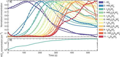
The chemical composition and the time evolution of the charged iodic acid clusters were measured with a negative APi-TOF. We present the time evolution of the negatively charged iodic acid clusters in Figure 1a. Zero time corresponds to switching on the green light and initiating the photolysis of iodine and its subsequent oxidation. The oxidation processes lead to the formation of iodine oxides (I_xO_y) and oxoacids (HIO_y). Galactic cosmic rays trigger primary air ion production, which in turn produces iodate (IO₃^-) by collisions with iodic acid. The interaction between ions and iodine-containing molecules initializes IIN processes, which is followed by charged cluster growth. The composition of the measured anions from the monomer to the 11-mer is noted by different colors, as shown in the legend. The measurements show a distinct appearance for each cluster, with the concentration rising to a peak and then gradually decreasing due to the growth processes. The negatively charged iodine clusters appear sequentially, with the (n + 1)-mer appearing after the n-mer. This suggests that the measured I₂O₅ in the negatively charged clusters is from the condensation and conversion of two HIO₃ molecules, providing critical support to the mechanism proposed in an earlier study (Sipilä et al. 2016). If the direct condensation of I₂O₅ would contribute significantly to the ion-induced iodic acid nucleation, the time sequence of the negatively charged clusters would not display such a pattern, as (n + 2)-mer would form immediately from n-mer. Thus, we confirm that the (HIO₃)_0-1·(I₂O₅)_n·IO₃^- clusters measured in Sipilä et al. 2016 can indeed form from pure HIO₃ addition in the presence of IO₃^- core anions.

Figure 1. Example evolution of the time sequence of a single ion-induced nucleation experiment in the CLOUD chamber. The experimental conditions are 11 °C, 34% RH, 40 ppbv ozone and 8 (±6) pptv I₂ with green light on. (a) The concentrations of charged clusters are measured by an negative APi-TOF (circles joined by lines); model predictions are shown by smooth curves. They are normalized by the maximum and minimum of individual time series. The colors indicate the number of iodine atoms in the charged cluster. The chemical composition and number of iodine atoms in the charged clusters are listed in the legend with respect to colors. (b) HIO₃ concentration during the experiment. Time represents the elapsed time from the starting of the experiment in seconds.

Collision rate coefficient calculation from measurement data

In this section, we analytically derive two methods to calculate collision rate coefficients of charged iodic acid clusters and HIO₃ molecules. We use an appearance time method since it has already been successfully used to calculate particle growth rates (Lehtipalo et al. 2014) which are conceptually similar to cluster growth rates. Step-by-step derivations can be found in the SI Section 2 (SI2), and we describe only the key steps here.

In order to obtain analytical solutions, several assumptions have to be made. While the validity of these assumptions is detailed in the SI, we briefly list these assumptions here:

1. The HIO₃ concentration is constant.

2. The ion production rate is constant.

3. At t = 0, the synthetic air is assumed to be clean, without any ions or neutral HIO₃.

4. The collision rate coefficients are the same for all the charged clusters regardless of size.

5. Only the HIO₃ monomer condenses on the charged clusters, while the neutral clusters do not coagulate with the charged clusters.

6. Cluster scavenging processes including wall loss, dilution loss, ion recombination, condensation sinks and thermal evaporation are assumed to be negligible.

With these assumptions, the growth of the charged clusters can be represented by a set of differential equations as follows (3) $$\{\begin{array}{l}\genfrac{}{}{0pt}{}{\frac{d[e^{-}]}{dt}=Q=a_1\times [e^{-}]}{\frac{d[u_1]}{dt}=a_1\times [e^{-}]-a_1\times [u_1]}\hfill \\ \genfrac{}{}{0pt}{}{\frac{d[u_2]}{dt}=a_1\times [u_1]-a_1\times [u_2]}{\frac{d[u_3]}{dt}=a_1\times [u_2]-a_1\times [u_3]}\\ \genfrac{}{}{0pt}{}{\dots }{\frac{d[u_i]}{dt}=a_1\times [u_{i-1}]-a_1\times [u_i]}\end{array}$$(3) where the e^- is the primary negative ion which is produced by galactic cosmic rays (the primary negative ions include e.g., electrons and O₂^-); Q is the ion production rate; [u_i] is the concentration of the charged cluster i-mer; a₁ is [HIO₃] × k₁ where [HIO₃] is the concentration of neutral HIO₃ and k₁ is the collision rate coefficient.

Using MATLAB 2017 to analytically solve the differential equations, the primary ion is found to follow (4) $$\{\begin{array}{c}\left[e^{-}\right]=\frac{Q-{Q\mathrm{e}}^{{-a}_{1}t}}{a_1}\\ \frac{d\left[e^{-}\right]}{dt}={Q\mathrm{e}}^{{-a}_{1}t}\\ \frac{d^2\left[e^{-}\right]}{{dt}^2}=-{Qa}_1{\mathrm{e}}^{{-a}_{1}t}\end{array}$$(4)

For the charged clusters, we find (5) $$\{\begin{array}{l}[u_i]=\frac{{-Qe}^{{-a}_{1}t}[{-e}^{a_{1}t}i!+i!+\sum _{n=1}^{i-1}(a_1^n{t}^n\prod _{m=n+1}^{i}m)+a_1^i{t}^i]}{a_{1}i!}\\ \frac{d[u_i]}{dt}=\frac{{Qa}_1^i{t}^i{e}^{{-a}_{1}t}}{i!}\\ \frac{d^2[u_i]}{{dt}^2}=-\frac{{Qa}_1^i{t}^{i-1}{e}^{{-a}_{1}t}(a_{1}t-i)}{i!}\end{array}$$(5)

We note that since MATLAB can only analytically solve until the [u₅], we further summarized and generalized the results into (5).

We further find (as detailed in SI2) that a maximum production rate method (MPR) can provide the following analytical solution for the collision rate coefficients (6) $$t_{i+1,\mathit{max}}{-t}_{i,\mathit{max}}=\frac{1}{a_1}=\frac{1}{\left[{\mathrm{HIO}}_3\right]\times k_1}=\tau$$(6) where t_i,max is the time when the i-mer reaches its maximum net production rate (note the difference to the maximum concentration), and τ is the expected lifetime of a single i-mer as it grows to become an (i + 1)-mer.

However, this analytical method is not suitable for experimental data with poor time resolution. The calculation of t_i,max requires $\frac{d^2[u_i]}{d{t}^2}=0$ to be calculated, which can yield high uncertainties with noisy experimental data. Therefore, another form needs to be derived.

From Equation (5)(5) $$\{\begin{array}{l}[u_i]=\frac{{-Qe}^{{-a}_{1}t}[{-e}^{a_{1}t}i!+i!+\sum _{n=1}^{i-1}(a_1^n{t}^n\prod _{m=n+1}^{i}m)+a_1^i{t}^i]}{a_{1}i!}\\ \frac{d[u_i]}{dt}=\frac{{Qa}_1^i{t}^i{e}^{{-a}_{1}t}}{i!}\\ \frac{d^2[u_i]}{{dt}^2}=-\frac{{Qa}_1^i{t}^{i-1}{e}^{{-a}_{1}t}(a_{1}t-i)}{i!}\end{array}$$(5) , the concentration difference between (i + 1)- and i-mers at time t can be represented as (7) $$\mathrm{\Delta }\left[u_{i,i+1}\right]\left(t\right)=[u_i]\left(t\right)-\left[u_{i+1}\right]\left(t\right)=e^{{-a}_{1}t}Q\frac{t^{i+1}{a}_1^i}{\left(i+1\right)!}$$(7)

Where $\Delta [u_{i,i+1}]$ is the concentration difference between i- and (i + 1)-mers. Further derivations find that the time t_i+1,maxDiff when $\Delta [u_{i,i+1}]$ achieves its maximum is the same time as the time t_i+1,max, i.e. (8) $$t_{i+1,\mathit{maxDiff}}=t_{i+1,\mathit{max}}=\frac{i+1}{a_1}$$(8)

We name this method as maximum concentration difference method (MCD). This means that at a time when an i-mer reaches its maximum production rate, the concentration difference between the (i-1)- and i-mers is the largest. However, we note here that despite MCD and MPR methods arrive at the same points under the conditions assumed in this study, they are intrinsically different methods.

Finally, despite the fact that the 50% appearance time method (APP50) cannot achieve analytical solutions to calculate the collision rate coefficient, we use it to derive two parameters to show its level of fidelity in comparison to MCD and MPR methods. (9) $$L_i=\frac{i!\left({-e}^{i}i!+2i!+2\sum _{n=1}^{i-1}\left(i^n\prod _{m=n+1}^{i}m\right)+{2i}^i\right)}{2i!i^i}$$(9) (10) $$Y_i=\frac{-\left[{-e}^{i+L_i}i!+i!+\sum _{n=1}^{i-1}\left({\left(i+L_i\right)}^n\prod _{m=n+1}^{i}m\right)+{\left(i+L_i\right)}^i\right]}{e^{i+L_i}i!}$$(10)

In order to achieve close enough results to MCD and MPR methods, two conditions need to be satisfied: the difference between L_i+1 and L_i needs to be small and Y_i+1 is close enough to 0.5. We show in Figure S1 that while for i < 5, these two conditions are not well satisfied, for i ≥ 5, they are well satisfied. Thereby, we conclude that when i < 5, the APP50 method produces a certain level of inaccuracy, while when i ≥ 5, the APP50 method produces close enough results to MCD and MPR methods, under the conditions defined for the derivation.

The collision rate coefficient between the (i + 1)-mer cluster and HIO₃ molecule is therefore calculated according to (11) $$k_{i+1}=\frac{1}{[HI{O}_3{]}_{\text{avg}}\times (t_{i+1}-t_i)}$$(11) where t_i+1, t_i are the characteristic times (derived from MCD, MPR or APP50 methods) of the (i + 1)-mer and i-mer, and [HIO₃]_avg is the averaged HIO₃ concentration during the time interval [t_i+1, t_i].

In order to visualize the difference among the three methods, we made a test simulation using the PANDA520 model with the same assumptions as in the derivation above. The input parameters are (12) $$\{\begin{array}{c}\left[{\mathrm{HIO}}_3\right]=2\times {10}^7 {\mathrm{cm}}^{-3}\\ Q=2 {\mathrm{s}}^{-1}\\ k_1=2\times {10}^{-9} {\mathrm{cm}}^3{\mathrm{molecules}}^{-1}{\mathrm{s}}^{-1}\end{array}$$(12)

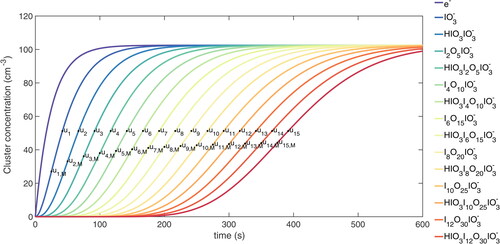
The results are shown in Figure 2. The MPR/MCD methods produce the points u_i,M, while the 50% appearance time method produces the points u_i. These two sets of points differ from each other, but with increasing i, the concentration differences decrease, as do the time differences between the neighboring points.

Figure 2. Schematic plot illustrating the difference between MPR/MCD and APP50 methods. The chemical composition and number of iodine atoms in the charged clusters are listed in the legend with respect to colors. u_i represents the APP50 points while u_i,M represents the MPR/MCD points.

A fundamental advantage shared by all three methods derived here is that they do not require charged cluster concentrations to calculate the collision rate coefficient. The characteristic times can be derived from normalized time series of individual charged clusters (Figure 2). This overcomes the difficulty that the number concentrations of atmospheric charged molecular clusters are only around 10-100 cm⁻³ at boundary layer conditions which are difficult to measure precisely. However, if concentrations of charged clusters can be measured precisely, for instance, under laboratory conditions, a simpler method can be found in e.g., Li et al. 2019.

Inter-comparison of the three methods

To test the accuracy of the three derived methods in calculating the collision rate coefficients, we treat the input collision rate coefficients in the PANDA520 model as the true values. After running the model, the time series of the charged clusters generated by the model are used to calculate the collision rate coefficients using the APP50, MCD and MPR methods. Two parameters are subjected to change in the comparison: the input collision rate coefficient and the HIO₃ concentration, while all other parameters stayed unchanged as described in the (SI).

In the first scenario, HIO₃ concentration is set to 2 × 10⁷ molecules cm⁻³ and all the collision rate coefficients are set to 2 × 10⁻⁹cm³ s⁻¹. This scenario is fairly similar to the simulation shown in Figure 2, except that all the loss and production processes are included in the simulation. The ratios between the calculated collision rate coefficients calculated by the three methods and the model input values are shown in Figure 3. The average over-estimations are 15%, 13% and 4% for APP50, MPR and MCD methods, respectively. We note that by the definition of the MCD method, the collision rate coefficient between IO₃^- and HIO₃ cannot be calculated. Thereby, the k₁ for the MCD method is not shown in the figure. In this scenario, all the three methods show good results, with the best estimation from the MCD method.

Figure 3. Comparison of the APP50, MPR and MCD methods under different experimental conditions. The y axis shows the ratio of the calculated collision rate coefficient to the model input. Different markers indicate different methods, as shown in the legend. (a) The HIO₃ concentration is 2 × 10⁷ molecules cm⁻³ and all the collision rate coefficients are set to 2 × 10⁻⁹cm³ s⁻¹. (b) The HIO₃ concentration is set to vary, the same trend as the HIO₃ concentration shown in Figure 1b. All the collision rate coefficients for odd number charged clusters are set to 2.5 × 10⁻⁹cm³ s⁻¹ and 1.5 × 10⁻⁹cm³ s⁻¹ for even number charged clusters. The missing values are negative values which the corresponding method fails to calculate.

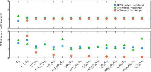
In the second scenario, the HIO₃ time series is input from the experiment shown in the Figure 1, i.e., it is increasing first then approaching a stable concentration. Additionally, the collision rate coefficient in the model is also set to vary. The collision rate coefficients for all the odd number charged clusters (e.g., monomer, trimer and so on) are set to 2.5 × 10⁻⁹cm³ s⁻¹, while the value is 1.5 × 10⁻⁹cm³ s⁻¹ for the rest. While this setting is not physically reasonable, it can, to a certain degree, mimic real atmospheric measurements in which data are not always smooth. Surprisingly, MCD method shows substantially worse results than the APP50 and MPR methods. Additionally, the APP50 method appears to be more stable against the MPR method.

Overall, the MCD method can achieve slightly better results when the real collision rate coefficients do not fluctuate, and when experimental conditions are more stable. On the other hand, the APP50 method has a more robust performance in the tested scenarios. Thus, we choose the APP50 method as the method to calculate the collision rate coefficient in this study. However, we note that in different applications, the MPR and the MCD methods could be more accurate, and thereby should not be discarded.

Collision rate coefficients between charged iodic acid clusters and iodic acid

The results of the collision rate coefficient calculated from the charged cluster appearance are shown in Figure 4. We note that since the iodate anion (IO₃^-) appears before the starting of our experiment, we cannot calculate the collision rate coefficients k₁ and k₂, according to Equation (11)(11) $$k_{i+1}=\frac{1}{[HI{O}_3{]}_{\text{avg}}\times (t_{i+1}-t_i)}$$(11) . This is because a small amount of residual HIO₃ was charged by natural anions because of its low proton affinity, causing an inaccurate estimation of the appearance time of the IO₃^-. The calculated collision rate coefficients have an average value of 2.4 × 10⁻⁹cm³ s⁻¹ with a standard variation of 8.2 × 10⁻¹⁰cm³ s⁻¹.

Figure 4. Collision rate coefficient calculated by the APP50 method and theoretical methods. The expected charged cluster collision rate coefficients from ADO theory are shown by the solid purple curve, values from HSA theory are shown by the solid pink line, values from the SCC method are shown by solid blue curve. The gray triangles are collision rate coefficients calculated by APP50 method based on the data shown in the Figure 1.

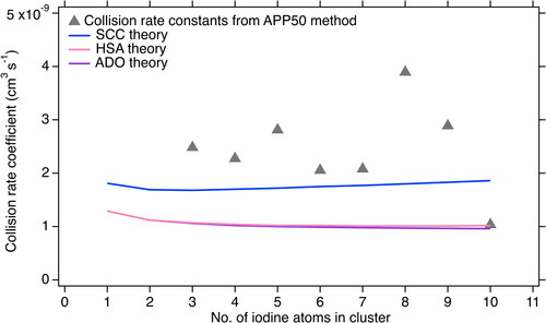
The collision rate coefficients calculated by ADO, HAS and SSC theories are also shown in Figure 4. The ADO and HSA theories produce similar results since the hard sphere collision assumption does not contribute significantly to the overall collision rate coefficient significantly. SCC theory produces much higher collision rate coefficients than the other two methods suggesting that if the charge is on the surface of the charged cluster, the rate coefficient can be enhanced (Kummerlöwe and Beyer 2005). Additionally, Ahonen et al. 2019 concluded that the hydration of charged iodic acid clusters increased the collision cross section by most 12% (up to saturation ratio of 0.65) which has a negligible effect on the overall collision rate coefficient. Our calculated collision rate coefficients are higher than all of the theoretical values, and closest to the SCC values. We further investigated the effect of wall loss and ion-ion recombination on the accuracy of the APP50 method as shown in the Figure S4. We find that, by including wall loss and ion-ion recombination into the model simulation, the calculated collision rate coefficients by the APP50 method are increased by 4% and 10%, respectively. This would suggest that the difference between the measured collision rate coefficients and the SCC theory values can partly arise from the error of the APP50 method. Nevertheless, as only one set of experimental data is used as an example case in this study, further investigations are needed to constrain the statistics and external losses on the accuracy of the proposed three methods.

Simulation of charged iodic acid cluster formation

Finally, we use the calculated collision rate coefficients as input in the PANDA520 model and try to simulate the measured charged iodic acid cluster formation processes shown in Figure 1. We note that theoretical values from the SCC theory are used for the missing collision rate coefficients that are not measured, since SCC theory produces results that are closest to our measured values. The initial total positive ion concentration was measured to be 806 ions cm⁻³, while the initial total negative ion concentration was 630 ions cm⁻³. The imbalance between the positive and negative ions is due to the NAIS ion detection size threshold and differences in the mobility size distributions of the initial positive and negative small ions. The anions are divided into “other negative ions” (377 molecules cm⁻³) and “IO₃^-” (253 molecules cm⁻³). This attribution is found empirically to fit the initial IO₃^- normalized ratio from the model to the APi-TOF measurement data (approximately 0.8) in Figure 1a by carrying out multiple simulations. Such attribution was made since we could not quantify the concentration of the measured charged clusters. However, since the APP50 method does not require charged cluster concentration as input values, the missing absolute concentrations do not affect the calculation of collision rate coefficients.

The results are shown by the solid lines in Figure 1a. We can see that the simulation reproduces the charged iodic acid cluster formation reasonably well, supporting the application of the APP50 method to calculate the collision rate coefficients. However, starting from the tetramer, our simulation seems to reach the maximum somewhat faster than the measured charged clusters. This implies that the application of the APP50 method may over-estimate the collision rate coefficients because the derivation of MCD, MPR, and APP50 methods neglects a number of loss and production processes.

Conclusion

In this study, we derived and evaluated three methods for the calculation of ion-polar molecule collision rate coefficients from the analysis of charged cluster appearance data. Of these, the 50% appearance time method is shown to be the most robust method, and it is thus chosen for our data analysis. With these methods, we are able to calculate the collision rate coefficient from the measured evolution of charged clusters and neutral molecules under atmospheric conditions. The collision rate coefficients have a mean value of (2.4 ± 0.8)×10⁻⁹cm³ s⁻¹ (1σ error). The enhanced collision rate coefficient, for charged clusters, together with their reduced evaporation rates, result in rapid growth of embryonic charged clusters, when they are especially vulnerable to scavenging loss. The results reported here are the first direct measurement of ion-polar molecule collision rate coefficients at atmospherically relevant conditions. In order to simulate charged iodic acid cluster formation processes, we further developed a kinetic model (PANDA520, see SI3) which accounts for all the cluster loss and formation processes in the CLOUD measurements. The simulation reproduces our measured charged iodic acid cluster appearance data reasonably well and validates our calculated collision rate coefficients. However, we note that future studies should account for the loss processes which are currently neglected in our derivation of the appearance time method.

Iodine-containing species have been measured globally (Saiz-Lopez et al. 2012), and iodic acid nucleation has been shown as an important process in coastal regions such as Mace Head, Ireland and Villum, Greenland (Sipilä et al. 2016). Given the threefold increase in atmospheric iodine over the past 70 years (Cuevas et al. 2018), the global contribution of ion-induced iodic acid nucleation is likely to continue to grow in future. However, despite its importance, ion-induced iodic acid nucleation is not yet included in global simulations. A part of the reason is that there is no quantitative information available to do so. The collision rate coefficients provided in our study can be used in global aerosol simulations to evaluate the contribution of ion-induced HIO₃ nucleation to regional and global new particle formation.

Acknowledgments

X.-C.H., S.I., V.-M.K, R.C.F., J.Kon., J.Kir., T.K. and M.K. wrote and/or edited the manuscript. X.-C.H., M.Sip., J.Kir. and M.K. designed the experiments. X.-C.H. and J.P. derived equations. X.-C.H. designed, wrote and ran the kinetic model. S.I., T.K. and X.-C.H. performed quantum chemical calculations. X.-C.H., A.Y., M.P., R.B., M.Sim. analyzed data. All other authors participated in either the development and preparations of the CLOUD facility and the instruments, and/or collecting and analysing the data.

Additional information

Funding

We thank the European Organization for Nuclear Research (CERN) for supporting CLOUD with important technical and financial resources and for providing a particle beam from the CERN Proton Synchrotron. This research has received supports from the Academy of Finland projects (316114, 307331, 310682, 266388, 306853, 296628, 299574, 326948); The European Research Council projects (692891, 616075, 764991, 316662, 742206, 714621); CSC – Finnish IT center; Austrian Science fund (FWF, J3951-N36, P27295-N20); the Swiss National Science Foundation (20FI20_159851, 200021_169090, 200020_172602, 20FI20_172622); the U.S. National Science Foundation Grants (AGS1447056, AGS1439551, AGS1801897, AGS1649147, AGS1801280, AGS1602086, AGS1801329); MSCA H2020 COFUND-FP-CERN-2014 fellowship (665779); German Federal Ministry of Education and Research: CLOUD-16 (01LK1601A); Academy of Finland Centre of Excellence in Atmospheric Sciences (grant no. 272041).

References

- Ahonen, L., C. Li, J. Kubecka, S. Iyer, H. Vehkamaki, T. Petäjä, M. Kulmala, and C. J. Hogan. 2019. Ion mobility-mass spectrometry of iodine pentoxide-iodic acid hybrid cluster anions in dry and humidified atmosphere. J. Phys. Chem. Lett. 10 (8):1935–41. doi:https://doi.org/10.1021/acs.jpclett.9b00453.
- Balaj, O. P., I. Balteanu, T. T. J. Roßteuscher, M. K. Beyer, and V. E. Bondybey. 2004a. Catalytic oxidation of CO with N2O on gas-phase platinum clusters. Angew. Chem. 116 (47):6681–4.
- Balaj, O. P., C.-K. Siu, I. Balteanu, M. K. Beyer, and V. E. Bondybey. 2004b. Reactions of hydrated electrons (H2O)n- with carbon dioxide and molecular oxygen: Hydration of the CO2- and O2- ions. Chemistry 10 (19):4822–30. doi:https://doi.org/10.1002/chem.200400416.
- Chai, J.-D., and M. Head-Gordon. 2008. Long-range corrected hybrid density functionals with damped atom-atom dispersion corrections. Phys. Chem. Chem. Phys. 10 (44):6615–20. doi:https://doi.org/10.1039/b810189b.
- Cuevas, C. A., N. Maffezzoli, J. P. Corella, A. Spolaor, P. Vallelonga, H. A. Kjaer, M. Simonsen, M. Winstrup, B. Vinther, C. Horvat, et al. 2018. Rapid increase in atmospheric iodine levels in the North Atlantic since the mid-20th century. Nat. Commun. 9 (1):1452. doi:https://doi.org/10.1038/s41467-018-03756-1.
- Dunning, T. H., and P. J. Hay. 1977. Gaussian basis sets for molecular calculations. In Methods of electronic structure theory, ed. H. F. Schaefer, 1–27. Boston, MA: Springer US.
- Feller, D. 1996. The role of databases in support of computational chemistry calculations. J. Comput. Chem 17 (13):1571–86.
- Friedlander, S. K. 2000. Smoke, dust, and haze: Fundamentals of aerosol dynamics. New York, NY: Oxford University Press.
- Frisch, M. J., G. W. Trucks, H. B. Schlegel, G. E. Scuseria, M. A. Robb, J. R. Cheeseman, G. Scalmani, V. Barone, B. Mennucci, G. A. Petersson, et al. 2009. Gaussian 09, revision D.01. Wallingford CT: Gaussian, Inc.
- Froyd, K. D., and E. R. Lovejoy. 2003. Experimental thermodynamics of cluster ions composed of H2SO4 and H2O. 2. Measurements and ab initio structures of negative ions. J. Phys. Chem. A 107 (46):9812–24.
- Fuentealba, P., H. Preuss, H. Stoll, and L. Von Szentpály. 1982. A proper account of core-polarization with pseudopotentials: Single valence-electron alkali compounds. Chem. Phys. Lett. 89 (5):418–22.
- Gordon, H., J. Kirkby, U. Baltensperger, F. Bianchi, M. Breitenlechner, J. Curtius, A. Dias, J. Dommen, N. M. Donahue, E. M. Dunne, et al. 2017. Causes and importance of new particle formation in the present-day and preindustrial atmospheres. J. Geophys. Res. Atmos. 122 (16):8739–60.
- Hu, S., and T. Su. 1986. Trajectory calculations of the effect of the induced dipole–induced dipole potential on ion–polar molecule collision rate constants. J. Chem. Phys. 85 (5):3127–8.
- Iyer, S., F. Lopez-Hilfiker, B. H. Lee, J. A. Thornton, and T. Kurtén. 2016. Modeling the detection of organic and inorganic compounds using iodide-based chemical ionization. J. Phys. Chem. A 120 (4):576–87. doi:https://doi.org/10.1021/acs.jpca.5b09837.
- Jokinen, T., M. Sipilä, H. Junninen, M. Ehn, G. Lönn, J. Hakala, T. Petäjä, R. L. Mauldin, M. Kulmala, and D. R. Worsnop. 2012. Atmospheric sulphuric acid and neutral cluster measurements using CI-APi-TOF. Atmos. Chem. Phys. 12 (9):4117–25. doi:https://doi.org/10.5194/acp-12-4117-2012.
- Junninen, H., M. Ehn, T. Petäjä, L. Luosujärvi, T. Kotiaho, R. Kostiainen, U. Rohner, M. Gonin, K. Fuhrer, M. Kulmala, et al. 2010. A high-resolution mass spectrometer to measure atmospheric ion composition. Atmos. Meas. Tech. 3 (4):1039–53., doi:https://doi.org/10.5194/amt-3-1039-2010.
- Kendall, R. A., T. H. Dunning, and R. J. Harrison. 1992. Electron affinities of the first‐row atoms revisited. Systematic basis sets and wave functions. J. Chem. Phys. 96 (9):6796–806.
- Kirkby, J., J. Curtius, J. Almeida, E. Dunne, J. Duplissy, S. Ehrhart, A. Franchin, S. Gagné, L. Ickes, A. Kürten, et al. 2011. Role of sulphuric acid, ammonia and galactic cosmic rays in atmospheric aerosol nucleation. Nature 476 (7361):429–33. doi:https://doi.org/10.1038/nature10343.
- Kirkby, J., J. Duplissy, K. Sengupta, C. Frege, H. Gordon, C. Williamson, M. Heinritzi, M. Simon, C. Yan, J. Almeida, et al. 2016. Ion-induced nucleation of pure biogenic particles. Nature 533 (7604):521–6., J. doi:https://doi.org/10.1038/nature17953.
- Kummerlöwe, G., and M. K. Beyer. 2005. Rate estimates for collisions of ionic clusters with neutral reactant molecules. Int. J. Mass Spectrom. 244 (1):84–90.
- Kürten, A., L. Rondo, S. Ehrhart, and J. Curtius. 2012. Calibration of a chemical ionization mass spectrometer for the measurement of gaseous sulfuric acid. J. Phys. Chem. A 116 (24):6375–86. doi:https://doi.org/10.1021/jp212123n.
- Lehtipalo, K., J. Leppä, J. Kontkanen, J. Kangasluoma, A. Franchin, D. Wimmer, S. Schobesberger, H. Junninen, T. Petäjä, and M. Sipilä. 2014. Methods for determining particle size distribution and growth rates between 1 and 3 nm using the Particle Size Magnifier. Boreal Environ. Res. 19 (suppl. B):215–36.
- Lehtipalo, K., L. Rondo, J. Kontkanen, S. Schobesberger, T. Jokinen, N. Sarnela, A. Kürten, S. Ehrhart, A. Franchin, T. Nieminen, et al. 2016. The effect of acid-base clustering and ions on the growth of atmospheric nano-particles. Nat. Commun. 7:11594. doi:https://doi.org/10.1038/ncomms11594.
- Li, C., M. Lippe, J. Krohn, and R. Signorell. 2019. Extraction of monomer-cluster association rate constants from water nucleation data measured at extreme supersaturations. J. Chem. Phys. 151 (9):094305 doi:https://doi.org/10.1063/1.5118350.
- Lushnikov, A. A., and M. Kulmala. 2005. A kinetic theory of particle charging in the free-molecule regime. J. Aerosol Sci. 36 (9):1069–88.
- Mackay, G. I., L. D. Betowski, J. D. Payzant, H. I. Schiff, and D. K. Bohme. 1976. Rate constants at 297 degree K for proton-transfer reactions with hydrocyanic acid and acetonitrile. Comparisons with classical theories and exothermicity. J. Phys. Chem. 80 (26):2919–22. doi:https://doi.org/10.1021/j100567a019.
- MATLAB. (2017). version 9.2.0 (R2017a). Natick, Massachusetts: The MathWorks Inc.
- O’Dowd, C. D., J. L. Jimenez, R. Bahreini, R. C. Flagan, J. H. Seinfeld, K. Hämeri, L. Pirjola, M. Kulmala, S. G. Jennings, and T. Hoffmann. 2002. Marine aerosol formation from biogenic iodine emissions. Nature 417:632–6.
- Saiz-Lopez, A., J. M. C. Plane, A. R. Baker, L. J. Carpenter, R. von Glasow, J. C. Gómez Martín, G. McFiggans, and R. W. Saunders. 2012. Atmospheric chemistry of iodine. Chem. Rev. 112 (3):1773–804. doi:https://doi.org/10.1021/cr200029u.
- Sakimoto, K. 1985. On the capture rate constant of collisions between ions and symmetric-top molecules. Chem. Phys. Lett. 116 (1):86–8.
- Sceats, M. G. 1989. Brownian coagulation in aerosols—the role of long range forces. J. Colloid Interface Sci. 129 (1):105–12.
- Sipilä, M., N. Sarnela, T. Jokinen, H. Henschel, H. Junninen, J. Kontkanen, S. Richters, J. Kangasluoma, A. Franchin, O. Peräkylä, et al. 2016. Molecular-scale evidence of aerosol particle formation via sequential addition of HIO3. Nature 537 (7621):532–4. doi:https://doi.org/10.1038/nature19314.
- Su, T. 1988. Trajectory calculations of ion–polar molecule capture rate constants at low temperatures. The Journal of Chemical Physics 88 (6):4102–3.
- Su, T., and M. T. Bowers. 1973a. Theory of ion‐polar molecule collisions. Comparison with experimental charge transfer reactions of rare gas ions to geometric isomers of difluorobenzene and dichloroethylene. J. Chem. Phys. 58 (7):3027–37.
- Su, T., and M. T. Bowers. 1973b. Ion-Polar molecule collisions: the effect of ion size on ion-polar molecule rate constants; the parameterization of the average-dipole-orientation theory. Int. J. Mass Spectrom. Ion Phys. 12 (4):347–56.
- Su, T., and W. J. Chesnavich. 1982. Parametrization of the ion–polar molecule collision rate constant by trajectory calculations. J. Chem. Phys. 76 (10):5183–5.
- Troe, J. 1987. Statistical adiabatic channel model for ion–molecule capture processes. J. Chem. Phys. 87 (5):2773–80.
- Vanommeslaeghe, K., E. Hatcher, C. Acharya, S. Kundu, S. Zhong, J. Shim, E. Darian, O. Guvench, P. Lopes, I. Vorobyov, et al. 2010. CHARMM general force field: A force field for drug-like molecules compatible with the CHARMM all-atom additive biological force fields. J. Comput. Chem. 31 (4):671–90. doi:https://doi.org/10.1002/jcc.21367.
- Viggiano, A. A., R. A. Morris, F. Dale, J. F. Paulson, K. Giles, D. Smith, and T. Su. 1990. Kinetic energy, temperature, and derived rotational temperature dependences for the reactions of Kr+(2P3/2) and Ar+ with HCl. J. Chem. Phys. 93 (2):1149–57.
- Viggiano, A. A., R. A. Morris, J. M. Van Doren, and J. F. Paulson. 1992. The effect of low frequency vibrations in CH4 on the rate constant for the reaction of O2+ (X 2Πg, v = 0) with CH4. J. Chem. Phys. 96 (1):275–84.
- Viggiano, A. A., R. A. Perry, D. L. Albritton, E. E. Ferguson, and F. C. Fehsenfeld. 1982. Stratospheric negative-ion reaction rates with H2SO4. J. Geophys. Res. 87 (C9):7340. doi:https://doi.org/10.1029/JC087iC09p07340.
- Zhang, J., and M. Dolg. 2015. ABCluster: the artificial bee colony algorithm for cluster global optimization. Phys. Chem. Chem. Phys. 17 (37):24173–81. doi:https://doi.org/10.1039/c5cp04060d.
- Zhang, J., and M. Dolg. 2016. Global optimization of clusters of rigid molecules using the artificial bee colony algorithm. Phys. Chem. Chem. Phys. 18 (4):3003–10. doi:https://doi.org/10.1039/c5cp06313b.