Effect of charge on aerosol microphysics of particles emitted from a hot wire generator: Theory and experiments

Abstract

The origin of ions in the lower atmosphere is attributed to sources like galactic cosmic rays, radioactive isotopes, gamma radiation, etc. These ions interact with atmospheric constituents affecting various atmospheric processes. Aerosol microphysical processes also get modified due to the presence of charge on particles. For aerosol generation, charging during generation and consequent effect on evolution dynamics is an important aspect. One of the efficient methods for the generation of nanaoparticle aerosols is via electrically heated wires i.e. hot wire generator (HWG). Although studies exist focusing on experimental insights, not much work has been performed in the direction of modeling the process for HWG systems. At present, there is a knowledge gap in the detailed understanding of charged aerosol microphysics of such high temperature systems. Models have been developed for different aspects of charged particles; but to the best of our knowledge, there are no studies which model the complete process for a hot wire generator, factoring both the effect of charge and Computational Fluid Dynamics (CFD). A CFD coupled aerosol microphysical model was developed for HWG in our earlier work. Charge has been added in the modified theoretical framework for the present work. The modified charged aerosol dynamic model has been coupled to the module for ion generation from hot sources. Thus, a newly developed CFD coupled charged aerosol microphysical model has been used for modeling the nanoparticle generation from HWG system. Results from the simulations have been compared with the experimental observations performed with a laboratory made HWG.

Copyright © 2021 American Association for Aerosol Research

EDITOR:

• Nicole Riemer

1. Introduction

Nanotechnology has great innovative and economic potential, and has, in recent years gained increasing significance. Nanoparticles (sizes less or equal to 100 nm) are drastically different than the corresponding bulk properties for any material. Nanoparticles have comparitively higher surface area and smaller volume. Consequently, the quantized conduction electrons are confined to a small volume, which allows them to interact with each other more effectively than larger particles (Khan et al. 2014). The properties of nanoparticles can be uniquely tuned by controlling its size, purity and crystallinity. This opens up various applications of nanoparticles, ranging from medicine, energy consumption and conversion, information technology to the chemical industry (Paschen et al. 2004). There are various reported methods for generation of nanoparticles in the laboratory. The most commonly used is wetchemistry (Brust et al. 1994; Giersig and Mulvaney 1993; Yonezawa and Kunitake 1999; Boies, Lvina, and Martens 2010). However, the use of solvents in this method leads to contamination of the particles and unwanted surface chemistry leading to impurities (Khan et al. 2014). Another method is nanoparticle generation through aerosols. It is achieved by gas-to-particle synthesis using furnace (Okuyama et al. 1989), flame (Pratsinis 1998), plasma (Kim 2005), laser reactors (Supronowicz et al. 2002), glowing wires (hot wire generator) (Peineke, Attoui, and Schmidt-Ott 2006), and spark discharges (Schwyn, Garwin, and Schmidt-Ott 1988), etc. This method provides the advantage of purity and crystallinity, compared to generation from liquids, due to the absence of solvents. Moreover, continuous production is more feasible in the gas phase.

Generation of nanoparticles from hot wire generator (HWG) is an efficient method, wherein a resistively heated wire is used to evaporate the material to gas phase (Schmidt-Ott, Schurtenberger, and Siegmann 1980). The gas vapors subsequently condense to form nanoparticle aerosols. The significant advantage of this method is that it offers a precise control over contamination (Peineke et al. 2009). Another advantage of this method of production of nanoparticle aerosols is the significantly higher number emission rates, which make them suitable for use in specific purposes such as validation of microphysics-based aerosol evolution models. However, due to the lack of measurment techniques, there is a knowledge gap in the detailed understanding of aerosol microphysics of HWG system, especially the nucleatioan process (of less than 3 nm size paticles) in earlier stages (Wang 2014). Also, chemical ionization and thermal ionization mechanisms (Fialkov 1997) lead to the generation of a high concentration of ions and charged clusters. Recent studies using sophisticated particle detectors showed that the fraction of charged species can be quite high for generation of aerosol from a high temperature source Wang, Vasaikar, et al. (2017). The ions and charged clusters lead to generation of charged nanoparticles in the system, which further changes the properties (such as size, shape, and crystallinity) (Novoselov et al. 2007; Shan et al. 2013; Li, Chahl, and Gopalakrishnan 2020). The characteristics of charge on the nanoparticles significantly effect the aerosol microphysics. For example, unipolar-ion environments has a different effect than bipolar ion environments (Vemury and Pratsinis 1995; Vemury and Pratsinis 1995; Zhang et al. 2011; Shan et al. 2013; Wang et al. 2016; Shen and Ren 2017). Measurements have also showed that positive ions had smaller mobilities than negative ions, resulting in higher fraction of negatively charged nanoparticles in the system Wang, (Kangasluoma, et al. 2017). Recently, we have studied the generation of vapors from HWG in detail (Ghosh et al. 2017), using aerosol microphysics coupled with Computational Fluid Dynamics (CFD). However the effect of particle charge was not incorporated in the developed theoretical framework.

The impact of charge in aerosol microphysics for different systems is demostrated in several studies (Kulmala, Pirjola, and Mäkelä 2000; Ghosh et al. 2017). Charge becomes extremely important when the particle size is less than 1 micrometer, especially for nano-size particles. This is because electrostatic force has a greater impact on smaller sizes compared to gravitational force, therefore charge becomes a key player in the aerosol microphysics of nanoparticles. Reported literature has also established that charge impacts significantly when the charge distribution is bipolar and ion concentration is greater than 10⁶ number/cc (Verheggen et al. 2007; Kulmala, Pirjola, and Mäkelä 2000). However, no studies have been conducted for a hot wire generator system. During the past few decades, a lot of interest has developed in ion-induced nucleation, which has resulted in new molecular based theories (Kusaka, Wang, and Seinfeld 1995) specifically dedicated to sign preference. Recent molecular works conclude that nucleation on negative ion is much stronger than positive because anionic clusters are more compact than cationic (Brodskaya, Lyubartsev, and Laaksonen 2002). Molecular theory and model simulations provide the understanding of sign preference nucleation and chemical nature of ions. Monte Carlo simulations on nucleation of water vapor reveals that anions are better nucleators because H⁺ prefers anions creating a considerable shorter anion-H distance (Oh, Gao, and Zeng 2001). Other studies (Kusaka, Wang, and Seinfeld 1995; Kusaka, Wang, and Seinfeld 1995) have concluded that size of the ions is also an important factor along with sign preference for nucleation (Kathmann, Schenter, and Garrett 2005). However, all models (Kusaka, Wang, and Seinfeld 1995; Kusaka, Wang, and Seinfeld 1995) results invariably reach the conclusion that water vapor prefers negative ions for nucleation. Another interesting result is that in certain cases, ion-induced nucleation is able to produce similar growth as observed in field experiments. The differences in the physical properties of positive and negative ions lead to in asymmetric charging, resulting in large difference in concentrations of positive and negatively charged particles. The governing particle sizes are inclined to establish a unique positive to negative ions ratio, which affects the steady state charge distribution of all other sizes. Therefore, for a polydisperse aerosol where ion concentrations are dictated by ion-aerosol attachment, the charge distribution will depend on the specific sizes of particles (Hoppel and frick). The production of charged nanoparticles from hot surfaces like glowing wires have been used earlier in connection with mobility classification, but the phenomenon is not well understood (Peineke and Schmidt-Ott 2008). To fully understand it, we have introduced charge dynamics module to the published CFD-aerosol microphysics (CFD-AM) HWG system model (Ghosh et al. 2020), to see the combined effects of charge and CFD on aerosol microphysics of HWG.

In this work, we have modified the CFD-AM by including ion effects in aerosol microphysics. This model uses the spatial profile of temperature and flow velocity around the glowing wire and incorporates them into aerosol microphyscis to develop a unique model to spatially simulate the genaration of charged particles from HWG. Dynamic implicit numerical scheme was used to solve mass, momentum and energy transfer in optimal time. Standard models for ion-induced nucleation (Lai and Nazaroff 2000; Pirjola et al. 1999; Raes and Janssens 1986), charge condensation (Lai and Nazaroff 2000), charged particle coagulation (Lai and Nazaroff 2000; Vohra et al. 2017; Ghosh et al. 2017) and electro static dispersion (Crump and Seinfeld 1981; Ghosh et al. 2017) have been used. The newly developed model (charge CFD-AM) has been validated with results obtained from experiments performed in laboratory-made HWG (Khan et al. 2014). SMPS have been employed to measure time evolution of integral number concentration ($\ge 4.5$ nm), size distribution ($5-350$ nm) and charged particle distribution with various sizes at the outlet (Joshi et al. 2012) of HWG cell. Relevant input parameters (such as temperature of wire and surrounding space in glowing condition, wire characteristics, etc.) have been measured and used for simulations. Thus, a complete aerosol microphysical model has been developed which is capable of simulating aerosol behavior accurately for high temperature aerosol generation sources. The inclusion of charge in an aerosol microphysical model, which also takes Computational Fluid Dynamics into account, has been achieved for the first time. In this regard, the work done in this is innovative and extremely important for any work that requires the understanding of aerosols. This model (charge CFD-AM), shown as validated CFD coupled with charge aerosol microphysics, can be used to understand the generation of charge from hot wire generator system or any other high temperature complex systems like car exhaust, chimneys, jet plume, plasma related application, etc.

2. Simulation methodology

In order to evaluate the generation, interaction and pathway of the charged particles in the HWG system, we used ion-induced nucleation model, charge condensation model, charge coagulation model and ion-induced deposition model; coupled with the CFD model, developed for HWG system:

2.1. Generation of ion and charge aerosol dynamics

The most recent theory for generation of charge inside a HWG chamber includes both positive and negative ion generation from high temperature source, as proposed by C. Peineke and A. Schmidt-Ott in 2007. Surface ionization theory predicts that many metallic materials show significant positive ion formation close to their melting temperature (Wahlin and Sordahl 1934). The flux of positive ions is obtained by evaporation rates of the material and charging efficiencies, the positive current density ($I_{+}$) described as (1) $$I_{+}(T_{\mathit{wire}})=e.\sum _{i=1}^n{E}_i(T_{\mathit{wire}}).B_i(T_{\mathit{wire}})$$(1)

where E_i can be described as (2) $$E_i=m_i.E_{\mathit{subs}}$$(2)

where m_i is used as two-component systems. The substrate and a species of significantly smaller ionization energy are represented by molar fractions of $(1-m_1)$ and m₁. In equation no. 1 B_i is the ionization probability of the i_th component and E_i represents the evaporation rate of the i_th component per unit surface area. The evaporation rate of the bulk material is given by the Hertz–Knudsen model described as (3) $$E_{\mathit{subs}}=\lambda {\left(\frac{N_a}{2\pi M_{\mathit{molar}}{K}_b{T}_{\mathit{wire}}}\right)}^{1/2}(P_{\mathit{sat}}(T_{\mathit{wire}})-P_o)$$(3)

λ is an accommodation coefficient to account for reduced evaporation due to reflection of vapor molecules from the surrounding atmosphere. N_a is Avogadro’s number, M_molar the molar mass and P_sat the saturation vapor pressure of species. Since, in the HWG the evaporated material is constantly transported away from the evaporation source, re-condensation on the wire is suppressed. This is accounted for by setting the vapor pressure in the surrounding atmosphere, P_o = 0.

At high temperatures thermal emission of electrons can generate negative ions in the system. The negative current density by the well-known Richardson equation can be described by (4) $$I_{-}=A.T_{\mathit{wire}}^2\hspace{0.17em}\text{exp}\hspace{0.17em}(-\frac{\varphi }{K_b{T}_{\mathit{wire}}})$$(4)

where $\varphi$ is the work function of the species, A can be described as (5) $$A=\frac{4\pi m_{\mathit{electron}}{K}_b^{2}e}{h^3}$$(5)

where m_electron being the electron mass and h being Planck’s constant. We assume that the evaporated material including ions completely nucleate to form charged and neutral particles. Thus, ion-aerosol interaction can be ignored as all ions formed are converted into charged particles through nucleation. The ion-induced nucleation rate is described in the following sections.

2.1.1. Equation for ion-induced nucleation

The possibility of ion induced nucleation increases drastically after generation of ions from the wire inside the chamber. For this phenomenon, the detailed ion induced nucleation model proposed by Kulmala (2002) has been used. This model is state-of-the-art as it includes all electrical forces: electrostatic coulomb, Van der Waals forces and image-forces. The simulated temperature (T_air) and vapor concentration (C) including ion concentration distribution from fluid dynamics model have been used for calculating nucleation rate (I_nu) expressed as (6) $$I_{nu}^q=R_{ab}{C}^{q}Z\hspace{0.17em}\text{exp}\hspace{0.17em}\left(\frac{-\mathit{delG}}{K{T}_{\mathit{air}}}\right)$$(6) where R_ab is the average condensation rate (Laakso et al. 2002), Z is the zeldowich nonequilibrium factor (Laakso et al. 2002), q denotes charge magnitude, K is the Boltzmann constant and delG is for nucleation barrier energy which can be expressed as (7) $$\mathit{delG}=\frac{-4\pi r_{\mathit{cri}}^{3}K{T}_{\mathit{air}}\hspace{0.17em}\text{log}\hspace{0.17em}S}{3v_{\mathit{mole}}}+4\pi \sigma r_{\mathit{cri}}^2+\frac{q^2}{8\pi {ϵ}_o}(1-\frac{1}{{ϵ}_r})\left(\frac{1}{r_{\mathit{cri}}}\right)$$(7) where v_mole is the molecular volume, σ is for surface tension of vaporized wire material (McNallan and Debroy 1991), S is the ratio between partial vapor pressure (P_surrounding) with saturation vapor pressure (Pvs) (Alcock, Itkin, and Horrigan 1984) and r_cri is the critical radius of nucleating charged and neutral particles. The critical radius generally this is taken as the first bin for the model. But, if the model predicted critical nucleation size is less than the molecular size of the evaporating material, then the molecular size is considered as the first bin. The r_cri can be described as (8) $$r_{\mathit{cri}}=\frac{2\sigma v_{\mathit{mole}}}{K{T}_{\mathit{air}}\hspace{0.17em}\text{log}\hspace{0.17em}S}[1-\frac{e^2(1-\frac{1}{{ϵ}_r})}{64{\pi }^2{ϵ}_o\sigma r_{\mathit{cri}}^3}]$$(8)

2.1.2. Charge condensation

The charge condensation rate is given by Laakso et al. (2002) can be calculated as (9) $$C_{\mathit{rate}}^q=F{c}_{\mathit{eff}}{N}_i^q{C}^q$$(9) where $C_{\mathit{rate}}^q$ is the charge condensation rate, F is the enhancment factor due to image force between vapor molecule and a charge particle, $N_i^q$ is the aerosol concentration and c_eff is the condensation coeeficient (Laakso et al. 2002).

2.1.3. Charge particle coagulation and ion induced deposition

Charge coagulation model is considered as collisions between neutral or charged particles and also ion collisions with aerosol particles, as described in (Laakso et al. 2002) and Ghosh et al. (2017). The charge coagulation term can be explained as (10) $$\frac{d{N}_i^q}{dt}=K{g}_{ij}^{mn}{N}_l^m{N}_j^n$$(10) where m, n refers to the charge and l, j to particle sizes. Coagulation coefficient $K{g}_{lj}^{mn}$ between the particles of size l and j. The updated coefficient for charged particle coagulation is given by (11) $$K{g}_{l,j}^{m,n}={\alpha }_{l,j}^{m,n}K{g}_{l,j}^B$$(11) where ${\alpha }_{l,j}^{m,n}$ is the correction due to charge and $K{g}_{l,j}^B$ is the particle Brownian coagulation coefficient. $K{g}_{l,j}^B$ includes all transition corrections as proposed by Fuchs Fuchs (1963). (12) $$K{g}_{l,j}^B=\frac{4\pi D_{l,j}{R}_{l,j}}{\frac{R_{l,j}}{R_{l,j}+{\delta }_{l,j}}+\frac{4D_{l,j}}{v_{l,j}+R_{l,j}}}$$(12)

The correction factor ${\alpha }_{l,j}^{m,n}$ was calculated from electrostatic, image and ion induced Van der Waal’s forces due to charge on particle in accordance with Ghosh et al.’s (2017) correction factor with respect to both size and charge was reformed as: (13) $${\alpha }_{l,j}^{m,n}=\hspace{0.17em}\text{exp}\left[\frac{-{\varphi }_{l,j}^{m,n}(r_m)}{KT}\right]$$(13)

In all other cases (valid for collision between neutral and charged particles also), the rearranged form will be (14) $${\alpha }_{l,j}^{m,n}=\frac{r_m^2(1-{\varphi }_{l,j}^{m,n}(r_m)/KT)}{R_{l,j}^2}$$(14) where $R_{l,j}$ is summation of R_l (radius of the particles for i size class) and R_j (radius of the particles for j size class). For repulsive case, in Equation (13)(13) $${\alpha }_{l,j}^{m,n}=\hspace{0.17em}\text{exp}\left[\frac{-{\varphi }_{l,j}^{m,n}(r_m)}{KT}\right]$$(13) r_m is the value where collision potential $\varphi$ becomes maximum. In Equation (14)(14) $${\alpha }_{l,j}^{m,n}=\frac{r_m^2(1-{\varphi }_{l,j}^{m,n}(r_m)/KT)}{R_{l,j}^2}$$(14) , r_m is the value where right hand side numerator reaches its minimum value. The collision potential $\varphi (r)$ is (15) $$\varphi (r_m)={\varphi }_{es}(r_m)+{\varphi }_{\mathit{img}}(r_m)+{\varphi }_{\mathit{vdw}}(r_m)$$(15) where ${\varphi }_{es}(r_m)$ is the collision potential for electrostatic force, ${\varphi }_{\mathit{img}}(r_m)$ is the collision potential for electrical image force and ${\varphi }_{\mathit{vdw}}(r_m)$ is the ion induced Van der Waals force described by Huang, Seinfeld, and Okuyama (1991), and further modified by Laakso et al. (2002) for multi sized particles.

The depositional losses due to diffusion, gravitational settling including electrostatic dispersion was described by Crump and Seinfeld (1981) and Ghosh et al. (2017). The loss rate for each grid can be calculated using the deposition velocities toward different surfaces as shown below. (16) $${\lambda }^I(p,U_I,t)=[A_{up}^I{v}_{up}^I(p,U_I,t)+A_{\mathit{down}}^I{v}_{\mathit{down}}^I(p,U_I,t)+A_{\mathit{side}}^I{v}_{\mathit{side}}^I(p,U_I,t)]/V_{\mathit{chamber}}^I$$(16) where λ^l is the particle deposition rate for each grid of the chamber; I denotes each grid of the chamber, A_up, A_down and A_side are the surface areas of the top, floor and walls of the each grid; v_up, v_down and v_side are the deposition velocities of particles calculated at respective portions of each grid. Corresponding v_side, v_top and v_floor details are described in Ghosh et al. (2017).

The newly formed charged particles are expected to condense and coagulate followed by deposition inside the chamber. For this process, the latest kernel for condensation, coagulation and deposition given by Jacobson has been used. This kernel is fast and provides a stable solution for any time step saving computational time compared to other available kernels. To account for the electrical factor, we have used the latest correction factor reported by Laakso et al. (2002) and our previously published work Ghosh et al. (2017).

2.2. Inclusion of CFD in the model

The inclusion of CFD for HWG case was necessary to validate the overall model results with experiments. The CFD model was chosen specially for natural convection case which was closest to the experimental set-up. The general flow dynamics of the HWG chamber was modulated using Navier-Stokes equation including buoyancy effects. The details of momentum, mass and energy balance equations are described in detail in the previous work of our group Ghosh et al. (2020). The complete flow (CFD) part of the model comprises of three major components: Rate of flow; vapor concentration and the temperature.

2.2.1. Calculation of rate of flow

The rate of flow is derived from the momentum equation as described in Ghosh et al. (2020). In this present context, the momentum equation has been modified to include buoyancy effect. The equation representing conservation of momentum for the present context as follows (17) $$\frac{\partial ({\rho }_{\mathit{air}}{u}_i)}{\partial t}+\frac{\partial ({\rho }_{\mathit{air}}{u}_i{u}_j)}{\partial x_i}=-\frac{\partial P}{\partial x_i}+\frac{\partial }{\partial x_i}\left({\mu }_{\mathit{eff}}\frac{\partial u_i}{\partial x_i}\right)+{\rho }_{\mathit{air}}{g}_i$$(17)

where P is the system pressure (same as atmospheric pressure here), $g_i\approx g$ is the acceleration due to gravity Last term used in Equation (17)(17) $$\frac{\partial ({\rho }_{\mathit{air}}{u}_i)}{\partial t}+\frac{\partial ({\rho }_{\mathit{air}}{u}_i{u}_j)}{\partial x_i}=-\frac{\partial P}{\partial x_i}+\frac{\partial }{\partial x_i}\left({\mu }_{\mathit{eff}}\frac{\partial u_i}{\partial x_i}\right)+{\rho }_{\mathit{air}}{g}_i$$(17) accounts for the buoyancy force under constant gravity. Effective viscosity (μ_eff) used in Equation (17)(17) $$\frac{\partial ({\rho }_{\mathit{air}}{u}_i)}{\partial t}+\frac{\partial ({\rho }_{\mathit{air}}{u}_i{u}_j)}{\partial x_i}=-\frac{\partial P}{\partial x_i}+\frac{\partial }{\partial x_i}\left({\mu }_{\mathit{eff}}\frac{\partial u_i}{\partial x_i}\right)+{\rho }_{\mathit{air}}{g}_i$$(17) can be expressed as the sum of viscosity of air (μ) and turbulent viscosity (μ_t) quantifying the contribution of turbulence in flow. The calculated flow is used in the dispersion and deposition parts of the complete aerosol dynamics. This is described in the following sections.

2.2.2. Calculation of vapor concentration

The vapor concentration is calculated using mass balance equation following the methods reported in Ghosh et al. (2020). The vapor concentration profile serves as the source term for aerosol formation and growth. Vapor concentration profile (source term for aerosol formation) in the cell can be obtained by solving mass transfer, i.e., advection-diffusion equation which is shown below: (18) $$\frac{\partial ({\rho }_{\mathit{air}}C)}{\partial t}+\frac{\partial ({\rho }_{\mathit{air}}{u}_{i}C)}{\partial x_i}=(\frac{\mu }{Sc}+\frac{{\mu }_t}{Sc})\frac{{\partial }^{2}C}{\partial x_i^2}+C_{\mathit{source}}-I_{nu}{n}_{cr}$$(18)

In this equation; C specifies the concentration of vapor molecules emitted from the heated wire material and Sc denotes the Schmidt number. The last two terms on the right hand side (RHS) are for vapor generation rate from the wire itself and loss rate due to nucleation process. The calculated vapor concentration is used in the nucleation and condensation parts of the complete aerosol dynamics model, described in the following sections.

2.2.3. Calculation of temperature

The electrical power supplied to the wire generates heat in the wire, which is the major source of temperature in the chamber. The temperature is calculated using the energy balance equation following the method reported in Ghosh et al. (2020). In this present context the energy balance equation used the input electrical power as the heat source term. Energy conservation equation for the present context has been written in terms of temperature as follows (19) $$\frac{\partial ({\rho }_{\mathit{air}}{T}_{\mathit{air}})}{\partial t}+\frac{\partial ({\rho }_{\mathit{air}}{u}_i{T}_{\mathit{air}})}{\partial x_i}=\frac{\partial }{\partial x_i}\left(\right(\frac{\mu }{Pr}+\frac{{\mu }_t}{P{r}_t}\left)\frac{\partial T_{\mathit{air}}}{\partial x_i}\right)+\frac{\partial Q_{\mathit{thi}}}{\partial t}$$(19) where T_air is the simulated air temperature and Q_th denotes the heat source term.The temperature profile is an integral part of the complete aerosol dynamics for comparison with experiments, chamber temperature was measured at various places using a K-type thermocouple.

2.3. General dynamics and transport equation of charged aerosol

Formation of charged aerosol particles, evolution of size spectrum and transport in the cell volume (including ion induced deposition on the surfaces) are mathematically expressed as the master equation (Pirjola et al. 1999; Raes and Janssens (1986) shown below, which combines ion induced nucleation model, charged coagulation model, charged condensation model, ion-induced deposition model and flow model developed for HWG system. (20) $$\begin{array}{c}\frac{\partial N_{I,l}^q}{\partial t}+\frac{\partial u_I{N}_{I,l}^q}{\partial x_i}=(D{p}_l+{\mu }_t)\left[\frac{{\partial }^2{N}_{I,l}^q}{\partial x_I^2}\right]+I_{nu}^q\frac{n_{cr}^I-n_{I,l-1}}{n_{I,l}-n_{I,l-1}}{f}_{n_{cr}^I,[n_{I,l-1},n_{i,l}]}+I_{nu}^q\frac{n_{i,l+1}-n_{cr}^i}{n_{i,l+1}-n_{i,l}}{f}_{n_{cr}^I,[n_{I,l},n_{I,l+1}]}\\ +\sum _{m,n=q_{\mathit{min}}}^{m,n=q_{\mathit{max}}}\sum _{j=1}^l\sum _{k=j}^l\frac{{\delta }_{m+n,q}^{I}K{g}_{j,k}^{m,n}(I)}{(1+{\delta }_{j,k}^I)(1+{\delta }_{m,n}^I)}{N}_{I,j}^m(t)N_{I,k}^n(t)-N_{I,l}^q(t)\sum _{m=1}^{N_c}\sum _{j=1}^{\mathit{nclass}}K{g}_{l,j}^{q,m}(I)N_{I,j}^m(t)-N_{I,l}^q(t){\lambda }_{I,l}^q\end{array}$$(20)

In above equation x_I represents directional coordinate for X and Y and N_I represents corresponding number concentration. Second term in LHS and first term in RHS quantify aerosol transport due to advection and diffusion. Second and third term in RHS are for particle formation due to nucleation (Laakso et al. 2002). The next two terms are for charge particle coagulation (Ghosh et al. 2017; Vohra et al. 2017). In above formulation Kg is the coagulation coefficient, j,k represent size classes of the coagulating particles and l represents the updated size after coagulation (j,k,l covering entire size range), n_cr is the critical number of molecule for nucleation, nclass means the final size class of the size distribution, f is the delta function for the case of nucleation, similar to that of coagulation. The coagulation terms used in above equation also allows the interaction of monomer with l-mer. Kronecker’s delta function for the case of coagulation with respect to size can be described as (21) $${\delta }_{n_j+n_k,[n_l,n_{l+1}]}=\{\begin{array}{cc}0,\hfill & n_j+n_k\ne [n_l,n_{l+1}]\hfill \\ 1,\hfill & n_j+n_k=[n_l,n_{l+1}]\hfill \end{array}$$(21)

$K{g}_{i,j}^{m,n}$ is charge coagulation coefficient, N_c is the number of bins for charge categories, q is the new charge category arising due to coagulation between two model charge categories l and m. ${\delta }_{m,n}$ and ${\delta }_{m+n,q}$ are the Kronecker delta function with respect to charges, given by (22) $${\delta }_{m+n,q}=\{\begin{array}{cc}0,\hfill & m+n\ne q\hfill \\ 1,\hfill & m+n=q\hfill \end{array}$$(22) (23) $${\delta }_{m,n}=\{\begin{array}{cc}0,\hfill & m\ne n\hfill \\ 1,\hfill & m=n\hfill \end{array}$$(23)

The last right hand side term of the Equation (20)(20) $$\begin{array}{c}\frac{\partial N_{I,l}^q}{\partial t}+\frac{\partial u_I{N}_{I,l}^q}{\partial x_i}=(D{p}_l+{\mu }_t)\left[\frac{{\partial }^2{N}_{I,l}^q}{\partial x_I^2}\right]+I_{nu}^q\frac{n_{cr}^I-n_{I,l-1}}{n_{I,l}-n_{I,l-1}}{f}_{n_{cr}^I,[n_{I,l-1},n_{i,l}]}+I_{nu}^q\frac{n_{i,l+1}-n_{cr}^i}{n_{i,l+1}-n_{i,l}}{f}_{n_{cr}^I,[n_{I,l},n_{I,l+1}]}\\ +\sum _{m,n=q_{\mathit{min}}}^{m,n=q_{\mathit{max}}}\sum _{j=1}^l\sum _{k=j}^l\frac{{\delta }_{m+n,q}^{I}K{g}_{j,k}^{m,n}(I)}{(1+{\delta }_{j,k}^I)(1+{\delta }_{m,n}^I)}{N}_{I,j}^m(t)N_{I,k}^n(t)-N_{I,l}^q(t)\sum _{m=1}^{N_c}\sum _{j=1}^{\mathit{nclass}}K{g}_{l,j}^{q,m}(I)N_{I,j}^m(t)-N_{I,l}^q(t){\lambda }_{I,l}^q\end{array}$$(20) is for wall deposition calculated using simulated velocity from K-Epsilon model, u_i, under the presence of gravity (Vohra et al. 2017). Particle diffusion coefficient (Dp) used above has been calculated from model temperature (T_air) and size of particles (d_p) (Rudyak 2013) as follows: (24) $$Dp=\frac{A+Q}{3\varphi }{N}_{AV}{\left(\frac{m_v}{2\pi }\right)}^{1/2}\frac{{(K{T}_{\mathit{air}})}^{3/2}}{{\rho }_{\mathit{air}}}\frac{1}{{(d_p)}^2}$$(24)

Where $\varphi$ is a constant depending gas molecule interaction (Rudyak, Dubtsov, and Baklanov 2009), N_AVis Avogadro’s number, d_p is the particle diameter and $(A+Q),$ the constant for modified Cunningham slip correction factor, described as (25) $$(A+Q)={(A+Q)}_0{\left(\frac{T_{\mathit{air}}}{T_0}\right)}^J$$(25) where ${(A+Q)}_0$ is the constant 1.657 and T₀ is 295, J is $\approx 1.6$ for particle diameter (d_p) less than $\approx 3.5nm$ and close to unity for particle diameter greater than $\approx 4nm.$

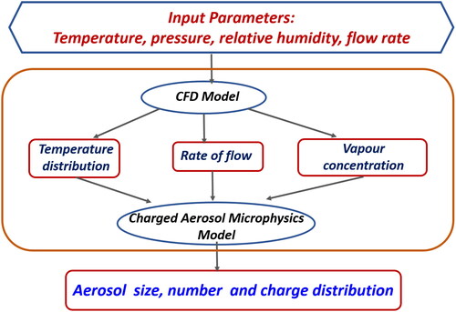
The overall model setup in the form of a schematic flow chart is show in Figure 1.

Figure 1. Schematic diagram showing the components of the developed model.

The model was computationally simulated in Matlab parallel software (2018 version) and validated with results described in Ghosh et al. (2020). MATLAB parallel scheme was used to save computation time. The CPU time is dependent on the number of cores available; for a 16 core processor it takes 10 min to simulate 1 h of simulation. All relevant parameters (system and process related) and constants used in the model are shown in Table 1.

Table 1. Parameters used for model calculation.

Item	Parameter name	Parameter value
Wire material	Length	0.03 m
	Mass	0.0011 Kg
	Inner diameter	0.011 m
	Input Power	10 & 30 Watt
	Specific heat capacity (cp)	450 $\text{Jule}{\text{Kg}}^{-1}{\mathrm{K}}^{-1}$
	Radiation coefficient (erad)	0.15 to 0.4, Makino, Kawasaki, and Kunitomo (1982)
	Thermal conductivity(Kthermal)	2.5 ${\text{Wm}}^{-1}{\mathrm{K}}^{-1}$
	Stefan boltzmann constant (erad)	$5.6\times {10}^{-8}$ ${\text{Wm}}^{-2}{\mathrm{K}}^{-4}$
Chamber dimension	Length	0.12 m
	Height	0.06 m
Model input	Smallest grid size	1 mm
	Growth factor for grid size	1.05, Rincón-Casado et al. (2017)
	Aerosol size bins	25, 50 and 100
	Aerosol size range	1 to 300 nm
	Aerosol charge bins	11
	Aerosol charge range	–5 to 5

2.4. Addition of charge to model setup and numerical scheme

Numerical simulations for the present case was performed for 2-dimension in terms of space along with three more dimensions (size of aerosol, charge of aerosol and time). This makes it a very time consuming simulation, and therefore, parallel computing and special numerical scheme was used for saving time. The HWG related modeling setup is the same as described in Ghosh et al. (2020). We have deployed variable mesh grid sizes in this system, using finer grid at the core and boundary, as most complex processes occur at the core or the boundary. A comparatively coarser grid size has been used for the other parts of the system. The complete flow with charge aerosol microphysics module is solved for all mesh grids, linking the different modules through time step. As all experimental measurements were obtained without external flow, model simulations have also been performed with the same conditions, i.e., considering only natural convection. Separate bins were added to deal with charges in the system. Charge particle generation mechanism (Wahlin and Sordahl 1934) was also introduced. Radiation coefficient (specifying radiation loss of wire in glowing condition) was taken from reported literature (Ghosh et al. 2020). The model simulations are performed for aerosol size distribution from 1 to 300 nm and charge ranges from −5 to +5. Higher charges have not been considered because most of the system particles are in nanometer size range with smaller surface volume causing low charge carrying capacities.

2.5. Validation of charge model sections for limiting cases

As the previously developed model is already complex involving fluid as well as particle dynamics, it is important to validate it for charge module separately before including the charge sub-modules, by either taking specific cases or against published results. These sub-modules include particle ion induced nucleation, charge condensation, charge particle coagulation and ion induced deposition. The ion induced nucleation and charge condensation scheme used in the developed model was validated against results of the model discussed by Laakso et al. (2002). The formulations used for charge particle coagulation and electrostatic dispersion (ion induced deposition) have been validated with results from our previously reported work (Ghosh et al. 2020). Grid independency test was performed again with the new model setup for output variables viz. number concentration, number size distribution and charge size distribution at the outlet of the generator.

3. Experimental layout

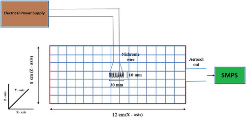
The experimental layout is similar to our previously reported work (Ghosh et al. 2020). Figure 2 shows the schematic diagram of the set-up. Three different power levels (10, 20 and 30 Watt) were used for study cases and th required power was maintained using constant power supply to the glowing wire. For comparison with newly developed charge model simulated results, GRIMM SMPS (scanning mobility particle sizer) was employed for measuring number size (5–350 nm in 45 size channels) distribution. The instrument can measure up to a maximum concentration in photometric mode of 10⁷ particle number/cm³. Six experiments were performed in controlled condition in HWG chamber and no external flow was used during the experiments, except the sampling flow (0.3 lpm) of instruments.

Figure 2. Schematic diagram showing the experimental layout of the chamber setup used for particle generation from HWG system.

4. Results and discussion

4.1. Charged aerosol model characteristics

The charge aerosol dynamics model developed here predicts the ion generation rate inside the chamber. Using Equation (1) and (4), the ion generation rate for each component of the the wire can be simulated and their sum as a function of the weighted mass can be obtained. These ions have been used in ion induced nucleation for generation of charged particles. Figure 3 shows the ion concentration change of different types of ions (Ni and Cr), with increasing wire temperature.

Figure 3. Ion concentration change with increasing wire temperature.

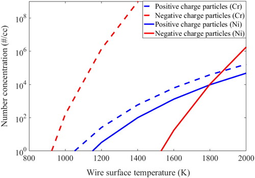
The red line denotes the model simulated values for negative ions and the blue line shows the positive ions concentration. It is clearly understandable that negative ion concentration increases with temperature due to thermal emission. The phenomena is well described in literature (Wahlin 1929). At the melting point of Ni (approx. 1800 K), there is a 10 order difference between positive ions of Cr and Ni; and a larger difference is observed for negative ions of Cr and Ni. This shows that, even at the reachable upper temperature limit of Ni, Cr ions dominate in the system. Therefore, Cr ions more heavily influence the final charge and size distribution of the HWG generated particle, for this type of wire used. It is also clearly observable in the figure that the overall concentration of negative ions is much higher than positive ions. This creates a bipolar environment in the chamber. The charged particle distribution has also been studied for bipolar and Boltzmann cases, to compare the bipolar charge influence in coagulation as against Boltzmann case for the Hot wire system.

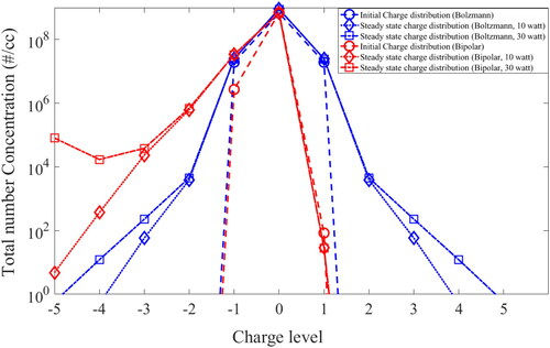
Figure 4 shows the charge particle distribution for different input powers (10 watt and 30 watt) as well as different charge case (bipolar and Boltzmann). The simulated charge distribution at 10 sec from start of simulation time is considered as the initial distribution (denotes as red and blue circles). The steady state charge distribution (denotes by red and blue squares) indicates a higher concentration of negatively charged particles for bipolar charge case compared to Boltzmann case, for both 10 and 30 watts input power. A possible reason for this is the larger number of negative ions generated at higher temperatures for bipolar charge case as shown in Figure 3. The continuous emission of bipolar ions leads to more negative charged particles in the system. This bipolar charge distribution affects the coagulation and deposition process significantly, which shows marked improvement in the results compared to neutral case. The details of the charge effect is discussed in Section 4.3.

Figure 4. Steady state charge distribution in HWG cell: charged and without charged case.

4.2. Flow dynamics model results

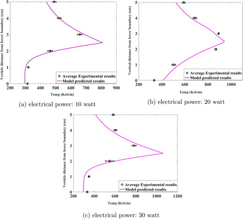
The previously developed CFD-AM model was used to calculate the essential characteristics of fluid flow namely velocity, temperature, density and viscosity. Accurate prediction of spatial temperature profile is crucial as it is directly linked to generation of charged aerosol in the system and its microphysics (Laakso et al. 2002; Pirjola et al. 1999). For the case of charge aerosol formation through electrically heated wire surface, surface ionization process takes place due to high surface temperatures, generating positively charged particles. High temperature also leads to thermal emission of electrons, which is the major sources of negatively charged particles in the system. This introduces highly charged aerosols in the system affecting the aerosol microphysics significantly, along with CFD driven forces. Here we are going to discuss some of the key outcomes of the developed charge model in terms of temperature, velocity and vapor profile as well as its effect on the charge dynamics. Model simulated steady state temperature profile in the chamber was compared with the measured temperature during the experiments. Figure 3 compares the average spatial temperature profile generated from six controlled experiments with results obtained from simulations performed with respect to the experimental conditions (electrical power supplied to the wire = 10, 20 and 30 watt). Temperature profile shown in this Figure 3 is for vertical line passing through the mid-plane of the glowing wire.

In Figure 5, average values for measured temperatures are plotted in black circles and in comparison, model simulation results are shown as red squares. The model predicted temperature values agree well with experimental observation. The temperature profile shown in this figure gives a clear indication of upward convection due to turbulence created by buoyancy effect. Such a non-homogeneous distribution of temperature results in nucleation zones very close to the wire surfaces which may lead to rapid formation of charged aerosol particles. Also, for the case of 30 and 20 watt, core temperature is much higher than for 10 watt input power, leading to more surface ionization and thermionic emission, resulting possibly in more bipolar charged particles. The relationship between temperature and charged particle generation rate is shown in Figure 3. The more detailed temperature related observations are discussed in previous published work (Ghosh et al. 2020).

Figure 5. Steady state spatial temperature profile in HWG cell: experimental measurements and simulations.

4.3. Comparison of model predictions and experimental observations

The results obtained from experiments described in Section 2 were compared against results from ’with charge’ and ’without charge’ model simulation. The experimental measurements for number concentration and number size distribution were performed only at the outlet of the hot wire chamber (see Figure 2). Therefore simulated results of only the boundary layer average grid (1 × 1 cm) was used for this comparison. The time series of total number concentration of charge (–5 to + 5) and without charged aerosol particles (greater than 4.5 nm to 300 nm size bins) for the two input power cases are shown in Figure 6.

Figure 6. Temporal evolution of total number concentration: experiments and simulations (charge vs. without charge).

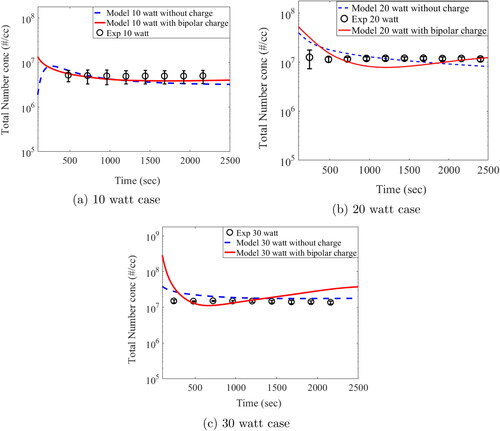
The red and blue lines in the above figure shows model predicted results for ‘charge’ and ‘without charge’ case respectively, while black circles represents the average number concentration measured during six experiments for each input power with error bars, calculated using one standard deviation. The model could predict the total number concentration reasonably well for both charged and without charged case. The major difference between charge and without charge case is found in initial time. The charge case shows more particles than without charge. The possible reason is that ion induced nucleation and charge particle coagulation increases the generation process of 5 nm particles. Investigating further, we have plotted (Figure 7) average size of the steady state distribution with different electrical power cases to determine the effect of charge and electrical power on the growth of particles.

Figure 7. Average size of particles in steady state condition for different power watt: experiments and simulations (charge vs. without charge).

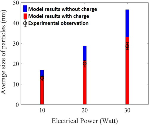
In this Figure 7, the blue bars are the results obtained from the without charge model and red bars are for with charge model for the different input power cases 10, 20, and 30 watt. The experimental results are shown as black circle with error bars. It is observed that with increasing input power, average particle sizes also increases. The increasing power results in rise of temperature at the wire surface, which leads to increasingly high vapor concentration in the system. As is clearly seen in Figure 7, the without charge model over predicts the average size for all input power cases, the difference significantly increasing with increase in input power. This can be explained by the fact that charge distribution suppresses the coagulation rate resulting in smaller size of average particles than that predicted by ‘without charge’ model. Further in the case of charge model, most of the particles are negatively charged as explained in Section 4.1 (Figure 4). This forms a modified bipolar or a pseudo-unipolar condition leading to a lower coagulation rate. The effect is more pronounced on increasing input power as the increasing temperature for each case results in higher initial concentration of charged particles in the system, as shown in Figure 3. This clearly indicates that the presence of charge in HWG system significantly affects the aerosol dynamics, more so for high input power cases. Experimental observations also support this claim as they match more closely with charged model results for all input power cases. Further, we also studied the comparison of particle size distribution evolution as shown in Figure 8.

Figure 8. Particle size distribution: model (charge and without charged) and experiments for (a) 10 watts, (b) 20 watts, and (c) 30 watts input power.

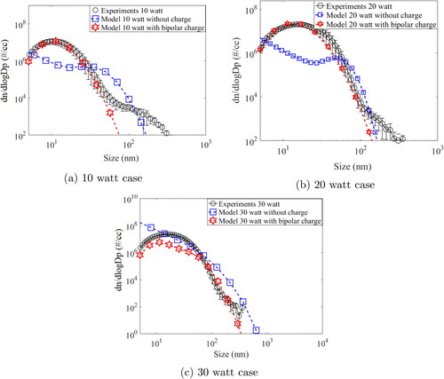
Figure 8 compares the steady state size distribution of aerosol particles at 10, 20, and 30 watt input power. For Figure 8a, the charged model prediction are remarkably close to experimental in comparison with without charge. For without charge case model is under performing could not capture the mode, however, for charge case model shows identical mode as in experiments. The major reason is that due to bipolar charge, the high concentration of nano size (less than 10 nm) particles enhance the coagulation process which changes the mode in comparison with without charge case. For higher sizes, ion induced deposition plays an important role in reducing particle number concentration. However the experiment results shows relatively more number concentration, possibly due to background initial concentration. For 8b, i.e., the without charge model gives mixed results, where it initially under-predicts and then over-predicts the number concentration. The charge model results shows an overall better agreement with the experimental results. However, the charged model also under predicts for sizes less than 100 nm. The same is seen for 8c, where. although the with charge model shows better agreement with experimental observations, it under-predicts for less than 100 nm particles. This indicates future scope for improvement of the model, like considering non-spherical particle coagulation. It is also observerd by Li and Gopalakrishnan (2021) that particle shape is important during diffusion based charging which may result in slightly different steady state charge distribution compared to shpericle particles. The reason that sphericity is assumed in the current model is because the instruments used for experimental validation, i.e., SMPS, calculates the number size distribution based on the assumption that the particles are spherical in nature. Since the model is being compared with the experimental observations, the same assumption has been followed in the model.

5. Conclusion

This work discusses the addition of much needed charge aerosol microphysics module in already developed CFD-AM model which can be used to understand charge effect for high temperature aerosol source systems. The model has been used to study evolution of number concentration, size and charge distribution of nanoparticles generated from glowing wire. The developed model was tested against previously published experimental results. Incorporation of charge module in CFD-AM provides the most realistic model setup for studying this type of system or application. Several experimental studies have been performed for flame generated particles that mentions the system as highly bipolar charged (Wang, Sharma, et al. 2017). The charge-CFD-AM model simulations for steady state charge distribution shows similar results. This well validates the newly developed charge-CFD-AM model and allows to gain knowledge on aerosol behavior for this type of systems. Model simulations showed significant of effect charge on aerosol microphysics, although the production rate of charge particles was very low. It was observed that in presence of constant source of ion (charged particle), steady state aerosol size and number distribution are certainly effected by charge aerosol microphysics. This proves that the idea of inclusion of ion in the understanding of high temperature sources or in atmosphere cloud dynamics model is much needed. In the previous published work (Ghosh et al. 2020), it was already presented how fluid properties effect the dynamics of aerosol particles. Specially the role of buoyancy was highlighted by observation and also through modeling studies. However, it was observed for the case of steady state number size distribution, there was reasonable differences between previous without charge model (CFD-AM) and experimental results for higher size ranges. Now with this improved model (charge-CFD-AM) results we have found good agreement with experimental results for all size ranges, showing a clear marked improvement in the model by inclusion of charge. With this improvement the present model becomes the most advanced model for high temperature aerosol generation systems to the best of our knowledge. It can also be used for diverse applications, e.g., emission of particles from hot surfaces (chimneys, car exhaust, jet plum), forest fires, biomass burning and interaction between atmospheric cloud with GCR (Galactic Cosmic Rays).

Nomenclature

Bi	=	positive charge efficiency
Bi	=	positive charge efficiency
Ei	=	evaporation rate
Ei	=	evaporation rate
$A_{up,\mathit{side},\mathit{down}}$	=	surface area
C	=	vapor concentration
delG	=	Gibbs free energy
Dpl	=	particle diffusion coefficient
g	=	acceleration due to gravity
$I_{+}$	=	positive ion
$I_{+}$	=	positive ion
$I_{-}$	=	negative ion
$I_{-}$	=	negative ion
Inu	=	nucleation rate
K	=	Boltzmann constant
K	=	Boltzmann constant
Kg	=	coagulation coefficient
l, j	=	size bins
mv	=	mass of gas molecule
N	=	aerosol concentration
N AV	=	Avogadro’s number
ncr	=	critical number for nucleation
Nsl	=	source of particles
P	=	chamber pressure
Qth	=	source of heat
Rab	=	average condensation rate
rcri	=	critical radius
$R_{l,j}$	=	summation between two colliding particle radius
S	=	saturation ration
Sc	=	Schmidt number
T	=	temperature
Vchamber	=	chamber volume
vmole	=	molecular volume of wire material
$v_{up,\mathit{side},\mathit{down}}$	=	deposition velocities on surfaces
α	=	correction factor due to charge
${\delta }_{m,n}$	=	Kronecker delta function with respect to charges
λ	=	particle deposition rate
μ	=	air viscosity
μeff	=	effective viscosity
$\varphi (r_m)$	=	collision potential due to charge on particles
λl	=	particle deposition rate
σ	=	surface tension

Acknowledgments

The present study was supported in part by Health, Safety and Environmental group, Bhabha Atomic Research Center, Government of India. Authors are thankful to Pallavi Khandare and Amruta Nakhwa for providing help during experiments. The authors gratefully acknowledge the financial support provided by Board of Research in Nuclear Science (BRNS), Department of Atomic Energy (DAE), Government of India to conduct this research under project no. 36(2,4)/15/01/2015-BRNS.

Additional information

Funding

The present study was supported in part by Health, Safety and Environmental group, Bhabha Atomic Research Center, Government of India. Authors are thankful to Pallavi Khandare and Amruta Nakhwa for providing help during experiments. The authors gratefully acknowledge the financial support provided by Board of Research in Nuclear Science (BRNS), Department of Atomic Energy (DAE), Government of India to conduct this research under project no. 36(2,4)/15/01/2015-BRNS.

References

- Alcock, C., V. Itkin, and M. Horrigan. 1984. Vapour pressure equations for the metallic elements: 298–2500k. Can. Metall. Q. 23 (3):309–13. doi:10.1179/cmq.1984.23.3.309.
- Boies, K., E. Lvina, and M. L. Martens. 2010. Shared leadership and team performance in a business strategy simulation. J. Personnel Psychol. 9 (4):195–202. doi:10.1027/1866-5888/a000021.
- Brodskaya, E., A. P. Lyubartsev, and A. Laaksonen. 2002. Investigation of water clusters containing oh-and h3o + ions in atmospheric conditions. A molecular dynamics simulation study. J. Phys. Chem. B 106 (25):6479–87. doi:10.1021/jp012053o.
- Brust, M., M. Walker, D. Bethell, D. J. Schiffrin, and R. Whyman. 1994. Synthesis of thiol-derivatised gold nanoparticles in a two-phase liquid–liquid system. J. Chem. Soc., Chem. Commun. 7:801–2. doi:10.1039/C39940000801.
- Crump, J. G., and J. H. Seinfeld. 1981. Turbulent deposition and gravitational sedimentation of an aerosol in a vessel of arbitrary shape. J. Aerosol Sci. 12 (5):405–15. doi:10.1016/0021-8502(81)90036-7.
- Fialkov, A. B. 1997. Investigations on ions in flames. Prog. Energy Combust. Sci. 23 (5–6):399–528. doi:10.1016/S0360-1285(97)00016-6.
- Fuchs, N. 1963. On the stationary charge distribution on aerosol particles in a bipolar ionic atmosphere. Geofisica Pura e Appl. 56 (1):185–93. doi:10.1007/BF01993343.
- Ghosh, K., S. Tripathi, M. Joshi, Y. Mayya, A. Khan, and B. Sapra. 2017. Modeling studies on coagulation of charged particles and comparison with experiments. J. Aerosol Sci. 105:35–47. doi:10.1016/j.jaerosci.2016.11.019.
- Ghosh, K., S. Tripathi, M. Joshi, Y. Mayya, A. Khan, and B. Sapra. 2020. Particle formation from vapors emitted from glowing wires: Theory and experiments. Aerosol Sci. Technol. 54 (3):243–61. doi:10.1080/02786826.2019.1688758.
- Giersig, M., and P. Mulvaney. 1993. Preparation of ordered colloid monolayers by electrophoretic deposition. Langmuir 9 (12):3408–13. doi:10.1021/la00036a014.
- Huang, D. D., J. H. Seinfeld, and K. Okuyama. 1991. Image potential between a charged particle and an uncharged particle in aerosol coagulation—Enhancement in all size regimes and interplay with van der waals forces. J. Colloid Interface Sci. 141 (1):191–8. doi:10.1016/0021-9797(91)90314-X.
- Joshi, M., B. Sapra, A. Khan, S. Tripathi, P. Shamjad, T. Gupta, and Y. Mayya. 2012. Harmonisation of nanoparticle concentration measurements using GRIMM and TSI scanning mobility particle sizers. J. Nanopart. Res. 14 (12):1268. doi:10.1007/s11051-012-1268-8.
- Kathmann, S. M., G. K. Schenter, and B. C. Garrett. 2005. Ion-induced nucleation: The importance of chemistry. Phys. Rev. Lett. 94 (11):116104. doi:10.1103/PhysRevLett.94.116104.
- Khan, A., P. Modak, M. Joshi, P. Khandare, A. Koli, A. Gupta, S. Anand, and B. Sapra. 2014. Generation of high-concentration nanoparticles using glowing wire technique. J. Nanopart. Res. 16 (12):2776. doi:10.1007/s11051-014-2776-5.
- Kim, K. 2005. Plasma synthesis and characterization of nanocrystalline aluminum nitride particles by aluminum plasma jet discharge. J. Cryst. Growth 283 (3–4):540–6. doi:10.1016/j.jcrysgro.2005.06.018.
- Kulmala, M., L. Pirjola, and J. M. Mäkelä. 2000. Stable sulphate clusters as a source of new atmospheric particles. Nature 404 (6773):66–9. doi:10.1038/35003550.
- Kusaka, I., Z.-G. Wang, and J. Seinfeld. 1995. Ion-induced nucleation. II. Polarizable multipolar molecules. J. Chem. Phys. 103 (20):8993–9009. doi:10.1063/1.470089.
- Laakso, L., J. M. Mäkelä, L. Pirjola, and M. Kulmala. 2002. Model studies on ion-induced nucleation in the atmosphere. J. Geophys. Res. 107 (D20):AAC-5. doi:10.1029/2002JD002140.
- Lai, A. C., and W. W. Nazaroff. 2000. Modeling indoor particle deposition from turbulent flow onto smooth surfaces. J. Aerosol Sci. 31 (4):463–76. doi:10.1016/S0021-8502(99)00536-4.
- Li, L., H. S. Chahl, and R. Gopalakrishnan. 2020. Comparison of the predictions of langevin dynamics-based diffusion charging collision kernel models with canonical experiments. J. Aerosol Sci. 140 (105481):105481. doi:10.1016/j.jaerosci.2019.105481.
- Li, L., and R. Gopalakrishnan. 2021. An experimentally validated model of diffusion charging of arbitrary shaped aerosol particles. J. Aerosol Sci. 151 (105678):105678. doi:10.1016/j.jaerosci.2020.105678.
- Makino, T., H. Kawasaki, and T. Kunitomo. 1982. Study of the radiative properties of heat resisting metals and alloys: (1st report, optical constants and emissivities of nickel, cobalt and chromium). Bull. JSME 25 (203):804–11. doi:10.1299/jsme1958.25.804.
- McNallan, M., and T. Debroy. 1991. Effect of temperature and composition on surface tension in Fe-Ni-Cr alloys containing sulfur. MTB. 22 (4):557–60. doi:10.1007/BF02654294.
- Novoselov, K. S., Z. Jiang, Y. Zhang, S. Morozov, H. L. Stormer, U. Zeitler, J. Maan, G. Boebinger, P. Kim, and A. K. Geim. 2007. Room-temperature quantum hall effect in graphene. Science 315 (5817):1379. doi:10.1126/science.1137201.
- Oh, K., G. Gao, and X. C. Zeng. 2001. Nucleation of water and methanol droplets on cations and anions: The sign preference. Phys. Rev. Lett. 86 (22):5080–5083. doi:10.1103/PhysRevLett.86.5080.
- Okuyama, K., J.-T. Jeung, Y. Kousaka, H. V. Nguyen, J. J. Wu, and R. C. Flagan. 1989. Experimental control of ultrafine TiO2 particle generation from thermal decomposition of titanium tetraisopropoxide vapor. Chem. Eng. Sci. 44 (6):1369–1375. doi:10.1016/0009-2509(89)85010-9.
- Paschen, S., T. Lühmann, S. Wirth, P. Gegenwart, O. Trovarelli, C. Geibel, F. Steglich, P. Coleman, and Q. Si. 2004. Hall-effect evolution across a heavy-fermion quantum critical point. Nature 432 (7019):881–885. doi:10.1038/nature03129.
- Peineke, C., M. Attoui, R. Robles, A. Reber, S. Khanna, and A. Schmidt-Ott. 2009. Production of equal sized atomic clusters by a hot wire. J. Aerosol Sci. 40 (5):423–430. doi:10.1016/j.jaerosci.2008.12.008.
- Peineke, C., M. Attoui, and A. Schmidt-Ott. 2006. Using a glowing wire generator for production of charged, uniformly sized nanoparticles at high concentrations. J. Aerosol Sci. 37 (12):1651–1661. doi:10.1016/j.jaerosci.2006.06.006.
- Peineke, C., and A. Schmidt-Ott. 2008. Explanation of charged nanoparticle production from hot surfaces. J. Aerosol Sci. 39 (3):244–252. doi:10.1016/j.jaerosci.2007.12.004.
- Pirjola, L., M. Kulmala, M. Wilck, A. Bischoff, F. Stratmann, and E. Otto. 1999. Formation of sulphuric acid aerosols and cloud condensation nuclei: An expression for significant nucleation and model comprarison. J. Aerosol Sci. 30 (8):1079–1094. doi:10.1016/S0021-8502(98)00776-9.
- Pratsinis, S. E. 1998. Flame aerosol synthesis of ceramic powders. Prog. Energy Combust. Sci. 24 (3):197–220. doi:10.1016/S0360-1285(97)00028-2.
- Raes, F., and A. Janssens. 1986. Ion-induced aerosol formation in a h2o-h2so4 system—II. Numerical calculations and conclusions. J. Aerosol Sci. 17 (4):715–722. doi:10.1016/0021-8502(86)90051-0.
- Rincón-Casado, A., F. Sánchez de la Flor, E. Chacón Vera, and J. Sánchez Ramos. 2017. New natural convection heat transfer correlations in enclosures for building performance simulation. Eng. Appl. Comput. Fluid Mech. 11 (1):340–356. doi:10.1080/19942060.2017.1300107.
- Rudyak, V. Y. 2013. Viscosity of nanofluids. why it is not described by the classical theories. ANP. 02 (03):266–279. doi:10.4236/anp.2013.23037.
- Rudyak, V. Y., S. Dubtsov, and A. Baklanov. 2009. Measurements of the temperature dependent diffusion coefficient of nanoparticles in the range of 295–600k at atmospheric pressure. J. Aerosol Sci. 40 (10):833–843. doi:10.1016/j.jaerosci.2009.06.006.
- Schmidt-Ott, A., P. Schurtenberger, and H. Siegmann. 1980. Enormous yield of photoelectrons from small particles. Phys. Rev. Lett. 45 (15):1284–1287. doi:10.1103/PhysRevLett.45.1284.
- Schwyn, S., E. Garwin, and A. Schmidt-Ott. 1988. Aerosol generation by spark discharge. J. Aerosol Sci. 19 (5):639–642. doi:10.1016/0021-8502(88)90215-7.
- Shan, Q., Y. Wang, K. Chen, Z. Liang, J. Li, Y. Zhang, K. Zhang, J. Liu, D. F. Voytas, X. Zheng, et al. 2013. Rapid and efficient gene modification in rice and brachypodium using talens. Mol. Plant. 6 (4):1365–1368. doi:10.1093/mp/sss162.
- Shen, M., and X. Ren. 2017. Highlights on immune checkpoint inhibitors in non-small cell lung cancer. Tumour Biol. 39 (3):1010428317695013. doi:10.1177/1010428317695013.
- Supronowicz, P., P. Ajayan, K. Ullmann, B. Arulanandam, D. Metzger, and R. Bizios. 2002. Novel current-conducting composite substrates for exposing osteoblasts to alternating current stimulation. J. Biomed. Mater. Res. 59 (3):499–506. doi:10.1002/jbm.10015.
- Vemury, S., and S. E. Pratsinis. 1995. Self-preserving size distributions of agglomerates. J. Aerosol Sci. 26 (2):175–185. doi:10.1016/0021-8502(94)00103-6.
- Verheggen, B., M. Mozurkewich, P. Caffrey, G. Frick, W. Hoppel, and W. Sullivan. 2007. Alpha-pinene oxidation in the presence of seed aerosol: Estimates of nucleation rates, growth rates, and yield. Environ. Sci. Technol. 41 (17):6046–6051. doi:10.1021/es070245c.
- Vohra, K., K. Ghosh, S. Tripathi, I. Thangamani, P. Goyal, A. Dutta, and V. Verma. 2017. Submicron particle dynamics for different surfaces under quiescent and turbulent conditions. Atmos. Environ. 152:330–344. doi:10.1016/j.atmosenv.2016.12.013.
- Wahlin, H. 1929. The emission of positive ions from metals. Nature 123 (3111):912–912. doi:10.1038/123912d0.
- Wahlin, H., and L. Sordahl. 1934. Positive and negative thermionic emission from columbium. Phys. Rev. 45 (12):886–889. doi:10.1103/PhysRev.45.886.
- Wang, J., S. Vasaikar, Z. Shi, M. Greer, and B. Zhang. 2017. Webgestalt 2017: A more comprehensive, powerful, flexible and interactive gene set enrichment analysis toolkit. Nucleic Acids Res. 45 (W1):W130–W137. doi:10.1093/nar/gkx356.
- Wang, L., Y. Xiong, Z. Wang, Y. Qiao, D. Lin, X. Tang, and L. Van Gool. 2016. Temporal segment networks: Towards good practices for deep action recognition. In European Conference on Computer Vision, 20–36. Springer.
- Wang, Y., J. Kangasluoma, M. Attoui, J. Fang, H. Junninen, M. Kulmala, T. Petäjä, and P. Biswas. 2017. The high charge fraction of flame-generated particles in the size range below 3 nm measured by enhanced particle detectors. Combust. Flame 176:72–80. doi:10.1016/j.combustflame.2016.10.003.
- Wang, Y., G. Sharma, C. Koh, V. Kumar, R. Chakrabarty, and P. Biswas. 2017. Influence of flame-generated ions on the simultaneous charging and coagulation of nanoparticles during combustion. Aerosol Sci. Technol. 51 (7):833–844. doi:10.1080/02786826.2017.1304635.
- Wang, Z. L. 2014. Triboelectric nanogenerators as new energy technology and self-powered sensors–Principles, problems and perspectives. Faraday Discuss. 176:447–458. doi:10.1039/C4FD00159A.
- Yonezawa, T., and T. Kunitake. 1999. Practical preparation of anionic mercapto ligand-stabilized gold nanoparticles and their immobilization. Colloids Surf. A. 149 (1–3):193–199. doi:10.1016/S0927-7757(98)00309-4.
- Zhang, Z.-Q., Q.-H. Fan, V. Pesic, H. Smit, A. V. Bochkov, A. Khaustov, A. Baker, A. Wohltmann, T. Wen, J. W. Amrine, et al. 2011. Order trombidiformes reuter, 1909. In: Zhang, z.-q.(ed.) animal biodiversity: An outline of higher-level classification and survey of taxonomic richness. Zootaxa 3148 (1):129–138. doi:10.11646/zootaxa.3148.1.24.