Optimal iteration and its application to some problems in aerosol science and particle dynamics

Abstract

Iteration is a common technique for finding the solutions to an equation. It is easy to code, straightforward to apply, readily comprehensible, and can be run indefinitely until a given accuracy is attained. However, for a given equation there are multiple iteration schemes that can be employed, with different convergence rates, and there is no obvious way to determine a priori which is best. Here the convergence rates of different approaches to simple iteration schemes are analyzed and the new technique of optimal iteration, which determines the scheme that maximizes the convergence rate, is introduced and illustrated by its application to several common problems in aerosol and particle dynamics. The first application is determination of the mobility diameter of an aerosol particle from the measured mobility, which is complicated by the nonlinearity of the Cunningham correction. This same equation occurs in the determination of the diameter of multiply charged particles with the same mobility diameter as singly charged particles. The next application is determination of the aerodynamic diameter from the mobility diameter for situations in which the Cunningham correction must be taken into account. The final two applications are determination of the terminal velocity from the diameter, and of the diameter from the terminal velocity, for particles sufficiently large that Stokes’ Law does not apply. The technique is easy to apply and can be employed in a number of situations.

Editor:

• Jim Smith

Introduction

Iteration is a common technique for finding a solution to an equation of the form (1) $$x=f\left(x\right)$$(1) in situations for which explicit solutions are not possible or not readily determined. Although other methods, including look-up tables, graphical methods, and root-solving routines like Newton’s Method can be employed to solve such equations, there are some instances where these other techniques are not viable or desirable, and where the simplicity and transparency of iteration makes it a common and useful option. The general principles are well known: an initial value, x₀, is chosen and substituted into the right side of Equation (1)(1) $$x=f\left(x\right)$$(1) to determine a value x₁, and this process is repeated indefinitely as successive values x_i+1 = f(x_i), where i is the number of the iteration, converge (hopefully) toward a value x_∞ that solves Equation (1)(1) $$x=f\left(x\right)$$(1) . However, different iteration schemes can be employed for the same equation, with different rates of convergence, and the choice of which is best is generally not obvious a priori.

This article introduces the technique of optimal iteration, which to the author’s knowledge has not previously been reported. This technique allows a priori determination of a simple iteration scheme from a given equation that yields the most rapid convergence. Here optimal iteration will be applied to several examples from aerosol dynamics: calculation of the mobility diameter of an aerosol particle from the measured mobility, calculation of the aerodynamic diameter of an aerosol particle, determination of the terminal velocity of a large particle from its diameter, and determination of the diameter of a large particle from its terminal velocity. Not only are these problems of interest in their own right, but also serve to demonstrate how the technique of optimal iteration can be applied to other situations. As these examples are selected to illustrate the power of this technique, only spherical particles will be considered, although the results could be extended to consider non-spherical particles for which a shape factor is required (Brockmann and Rader 1990; DeCarlo et al. 2004).

The outline of the manuscript is as follows. First, various iteration schemes for determination of the mobility diameter from the measured mobility will be presented. This is a familiar problem and thus will provide a framework that will facilitate understanding of the optimal iteration technique. Next, the convergence rate of an iteration scheme will be examined in general and the convergence rates the various schemes presented for the determination of the mobility diameter will be explained. This examination leads to the technique of optimal iteration: the scheme with the fastest convergence rate, which will be introduced for a general equation, and a geometric explanation for iteration will be presented. Optimal iteration will then be applied to the specific example of determination of the mobility diameter, and a technique for determining an accurate value for the initial value to begin iteration is presented. After this, various iteration schemes for the determination of the aerodynamic diameter will be presented and the technique of optimal iteration will be applied to this problem. Finally, optimal iteration will be applied to the determination of the terminal velocity from the diameter, and determination of the diameter from the terminal velocity, for a sphere sufficiently large that Stokes’ Law does not apply. A summary of the optimal iteration schemes and check values for each of the four cases are presented in the online supplementary information.

Example 1: Calculation of mobility diameter

The aerodynamic drag force, F_aero, on a spherical particle with diameter d moving through a gas at constant velocity u is typically given by Stokes’ Law (Stokes 1850), which states that this force is directly proportional to the velocity and to the diameter: F_aero = 3πµ_gdu, where µ_g is the dynamic viscosity of the gas. For sufficiently small particles, this expression must be reduced by a factor C, the Cunningham correction, which accounts for the discrete nature of the gas in which the particle is moving (Cunningham 1910; Millikan 1923) and depends on the ratio of the diameter of the particle to the mean free path of the gas, λ. The Cunningham correction is shown in Figure 1 for particles with mobility diameters from 1 to 1000 nm. Over this range it decreases from a very large value, approximately 2aλ/d_mob (where a is a constant near 1.65), at small mobility diameters to near unity for large mobility diameters (at 1000 nm, C ≈ 1.16). For the examples presented here, the formulation of Kim et al. (2005) is used: $C=1+\left(\frac{2\lambda }{d_{\text{mob}}}\right)\cdot \{1.165+0.483\cdot \hspace{0.17em}\text{exp}\hspace{0.17em}[-0.997\cdot \left(\frac{d_{\text{mob}}}{2\lambda }\right)]\}$ (although nothing in the analysis depends upon this specific choice), and a mean free path of 66.4 nm (Allen and Raabe 1982), the value for air at 20 °C and 1 atm, is assumed.

Figure 1. Cunningham correction, C, and its asymptotic value for low mobility diameter, d_mob, and X ≡ d_mob/C(d_mob), as functions of the mobility diameter. C is dimensionless, units for X are nm.

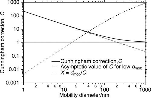
A typical problem in aerosol dynamics is determination of the mobility diameter of an aerosol particle, d_mob, from a measured mobility (e.g. Stolzenburg and McMurry 2008). This determination would be trivial but for the Cunningham correction. The equation to be solved in this situation, which is obtained by matching the drag force on the particle to the electrical force, is (2) $$\frac{d_{\text{mob}}}{C\left(d_{\text{mob}}\right)}=X,$$(2) or equivalently, d_mob = X·C(d_mob), for a given value of X that is inversely proportional to the measured mobility. This equation is in the form of Equation (1)(1) $$x=f\left(x\right)$$(1) , with x replaced by d_mob and with f(x) equal to X·C(d_mob). The relationship between X and the solution d_mob to Equation (2)(2) $$\frac{d_{\text{mob}}}{C\left(d_{\text{mob}}\right)}=X,$$(2) is shown in Figure 1. Another specific example that requires solution of this equation is the calculation of the diameter of a particle with charge q, d_mob^q, that has the same mobility diameter as that of a particle with a single charge, d_mob¹. In this case, X ≡ q·d_mob¹/C(d_mob¹), and the equation to be solved is d_mob^q/C(d_mob^q) = X.

There are many options for solving Equation (2)(2) $$\frac{d_{\text{mob}}}{C\left(d_{\text{mob}}\right)}=X,$$(2) , but most discussions of mobility diameter in the literature provide no details as to which is used. For instance, Mulholland, Bryner, and Croarkin (1999) and Kim et al. (2005) merely state that the equation is solved iteratively (Mulholland et al. 2006 does describe the iterative scheme employed, but this is an exception). One obvious iteration scheme is (3) $$d_{\text{mob},i+1}=X\cdot C\left(d_{\text{mob},i}\right).$$(3)

The solution to this equation for d_mob from 1 to 1000 nm is shown in Figure 2 as the percent difference of successive iterations from the actual value, for an initial value 50% greater than the solution. This initial value, although far greater than what would typically be used, and far greater than the initial value presented below, is selected here to better illustrate the convergence properties.

Figure 2. Percent differences from actual values of mobility diameter, d_mob, of the successive iterations using schemes given by Equation (3)(3) $$d_{\text{mob},i+1}=X\cdot C\left(d_{\text{mob},i}\right).$$(3) , black; Equation (4)(4) $$d_{\text{mob},i+1}={\left[d_{\text{mob},i}\cdot X\cdot C\left(d_{\text{mob},i}\right)\right]}^{\frac{1}{2}}.$$(4) , red; and Equation (5)(5) $$d_{\text{mob},i+1}={\left\{d_{\text{mob},i}\cdot X^2\cdot {\left[C\left(d_{\text{mob},i}\right)\right]}^2\right\}}^{\frac{1}{3}}.$$(5) , blue, as a function of mobility diameter.

This scheme converges rapidly for large particles. For example, successive iterations for mobility diameter 500 nm, starting with an initial value of 750 nm, are 460, 511, 497, and 501 nm. Successive iterations are alternately below and above the solution, and thus the fractional differences shown in Figure 2 are alternately negative and positive. However, convergence is very slow for smaller particles: successive iterations for mobility diameter 5 nm, starting with an initial value of 7.5 nm, are 3.35, 7.42, 3.39, and 7.35 nm. The values are again alternatively above and below the solution, but do not change much on alternate successive iterations. For intermediate sizes, the scheme yields slow convergence: for mobility diameter 50 nm, starting with an initial value of 75 nm, successive iterations yield 35.7, 67.5, 38.9, and 62.5 nm.

The convergence behavior of this scheme can be understood by noting that C is near unity for large mobility diameters, in which case the iterative scheme is nearly the same as d_mob = X. Conversely, as C is near 2aλ/d_mob for small mobility diameters, the iterative scheme is basically the same as d_mob = (2aλX)/d_mob, where the numerator is constant; thus successive iterations alternate between values below and above the actual value, and alternate iterations are roughly equal to the initial value in magnitude.

Another iteration scheme for Equation (2)(2) $$\frac{d_{\text{mob}}}{C\left(d_{\text{mob}}\right)}=X,$$(2) can be obtained by multiplying both sides of the equation by d_mob and taking the square root of both sides: (4) $$d_{\text{mob},i+1}={\left[d_{\text{mob},i}\cdot X\cdot C\left(d_{\text{mob},i}\right)\right]}^{\frac{1}{2}}.$$(4)

This approach is equivalent to taking the geometric mean of the right-hand side of Equation (3)(3) $$d_{\text{mob},i+1}=X\cdot C\left(d_{\text{mob},i}\right).$$(3) , X·C(d_mob), and d_mob (Mulholland et al. 2006 employ a similar technique but take the arithmetic mean of these two quantities). The results of this scheme over the same range of d_mob also shown in Figure 2, again as the percent difference of successive iterations from the actual value, with an initial value 50% greater than the solution. Convergence is extremely rapid for small particles, but slower for larger particles. For example, successive iterations for mobility diameter 5 nm, starting with an initial value of 7.5 nm, are 5.02 and 5.00009, whereas those for mobility diameter 500 nm, starting with an initial value of 750 nm, are 587, 532, 512, and 505 nm. For intermediate values of mobility diameter, convergence is also rapid. For instance, successive iterations for mobility diameter 50 nm, starting with an initial value of 75 nm, are 51.7, 50.1, and 50.008 nm. Convergence is monotonic for all mobility diameters. The rapid convergence of this scheme for small particles can be understood by noting that as C is nearly inversely proportional to d_mob for small mobility diameters, the quantity in brackets on the right side of Equation (4)(4) $$d_{\text{mob},i+1}={\left[d_{\text{mob},i}\cdot X\cdot C\left(d_{\text{mob},i}\right)\right]}^{\frac{1}{2}}.$$(4) is nearly constant.

Yet another scheme can be devised in which both sides of Equation (2)(2) $$\frac{d_{\text{mob}}}{C\left(d_{\text{mob}}\right)}=X,$$(2) are squared and then multiplied by d_mob, after which the cube root is taken: (5) $$d_{\text{mob},i+1}={\left\{d_{\text{mob},i}\cdot X^2\cdot {\left[C\left(d_{\text{mob},i}\right)\right]}^2\right\}}^{\frac{1}{3}}.$$(5)

The results of this scheme over a range of X, also shown in Figure 2 for initial values 50% greater than the solution, demonstrate that it yields rapid convergence over the entire range of d_mob considered. Successive iterations for mobility diameter 5 nm, with initial value 7.5 nm, are 4.39, 5.22, 4.93, and 5.02 nm; those for mobility diameter 500 nm, with initial value 750 nm, are 541, 507, 501, and 500.2 nm (monotonic convergence), and those for mobility diameter 50 nm, initially at 75 nm, are 45.7, 51.1, 49.7, 50.07 nm. The value after four iterations is within 0.5% of the actual over the entire range of mobility diameters considered, even for an initial value so far from the actual solution.

The various convergence properties of the different iteration schemes, Equations (3)(4) $$d_{\text{mob},i+1}={\left[d_{\text{mob},i}\cdot X\cdot C\left(d_{\text{mob},i}\right)\right]}^{\frac{1}{2}}.$$(4) , (4)(4) $$d_{\text{mob},i+1}={\left[d_{\text{mob},i}\cdot X\cdot C\left(d_{\text{mob},i}\right)\right]}^{\frac{1}{2}}.$$(4) , and (5)(5) $$d_{\text{mob},i+1}={\left\{d_{\text{mob},i}\cdot X^2\cdot {\left[C\left(d_{\text{mob},i}\right)\right]}^2\right\}}^{\frac{1}{3}}.$$(5) , for the same equation prompt several questions: What is it about the various schemes that yields the different convergence properties? Why does one scheme yield slow convergence in a given range of mobility diameter whereas another one does not? Why do some schemes yield values that are alternatively above and below the solution, whereas others converge monotonically? How would one have arrived at the third scheme, Equation (5)(5) $$d_{\text{mob},i+1}={\left\{d_{\text{mob},i}\cdot X^2\cdot {\left[C\left(d_{\text{mob},i}\right)\right]}^2\right\}}^{\frac{1}{3}}.$$(5) , which is rather non-intuitive, but yields rapid convergence? More to the point, what analysis can guide the search for an iteration scheme that performs best over a certain range? These questions will be addressed by first examining the convergence of iterative schemes in general, and then using these results to explain the different convergence properties of the three schemes used above to determine the mobility diameter. After that, the technique of optimal iteration will be introduced and described.

Analysis of convergence schemes

Analysis of the convergence of iterative schemes typically proceeds by writing the value at a given iteration, x_i, as x_i = x_∞ + ε_i, that is, as the sum of the actual value and a small difference, and substituting this expression into Equation (1)(1) $$x=f\left(x\right)$$(1) , which is then expanded in a Taylor series for which only first-order terms are retained. This approach makes the assumption that the initial guess, and all subsequent iteration values, are sufficiently close to the solution that higher-order terms can be neglected. In aerosol studies, however, there is generally a wide range of particle sizes considered, and it is not the difference, but rather the fractional difference, between a value x_i and the solution x_∞ that is the relevant quantity (for example, an inaccuracy of 2 nm between the value at a certain iteration step and the solution will have much greater consequences for a mobility diameter of 5 nm than for one of 500 nm). Thus, the above approach will be slightly modified to consider the fractional difference from the solution, and the value at a given iteration will be written as x_i = x_∞·(1 + ε_i), which will then be substituted into Equation (1)(1) $$x=f\left(x\right)$$(1) and expanded to yield $$x_{\mathrm{\infty }}\left(1+{\epsilon }_{i+1}\right)=f\left(x_{\mathrm{\infty }}\left(1+{\epsilon }_i\right)\right)=f\left(x_{\mathrm{\infty }}\right)+{\frac{df}{dx}|}_{x_{\mathrm{\infty }}}\cdot \left(x_{\mathrm{\infty }}{\epsilon }_i\right)+\dots =f\left(x_{\mathrm{\infty }}\right)\cdot \left\{1+{\left[\left(\frac{x}{f}\right)\cdot \left(\frac{df}{dx}\right)\right]|}_{x_{\mathrm{\infty }}}\cdot {\epsilon }_i+\dots \right\}.$$

Upon simplification, taking into account the fact that x_∞ = f(x_∞), the following result can be obtained for the convergence ratio, R_ε, the limit of the ratio of the fraction differences from the solution: (6) $$R_{\epsilon }\equiv \underset{i\to \infty }{\lim }\frac{{\epsilon }_{i+1}}{{\epsilon }_i}={\left[\left(\frac{x}{f}\right)\cdot \left(\frac{df}{dx}\right)\right]|}_{x_{\infty }}={\frac{d\hspace{0.17em}\text{ln}\hspace{0.17em}f}{d\hspace{0.17em}\text{ln}\hspace{0.17em}x}|}_{x_{\infty }}$$(6) (it is assumed here in taking the logarithm that f > 0, although the analysis could easily be extended to situations where f < 0). This result, that R_ε is equal to the derivative of the logarithm of the functional expression with respect to the logarithm of the independent variable, evaluated at the solution x_∞, is the key to answering the questions posed at the end of the last section. It is worth noting that as x_∞ = f(x_∞), the quantity dlnf/dlnx is equal to df/dx when both are evaluated at x_∞; however, use of the logarithmic derivative will prove more convenient in the analysis, as shown below.

The convergence ratio R_ε given by Equation (6)(6) $$R_{\epsilon }\equiv \underset{i\to \infty }{\lim }\frac{{\epsilon }_{i+1}}{{\epsilon }_i}={\left[\left(\frac{x}{f}\right)\cdot \left(\frac{df}{dx}\right)\right]|}_{x_{\infty }}={\frac{d\hspace{0.17em}\text{ln}\hspace{0.17em}f}{d\hspace{0.17em}\text{ln}\hspace{0.17em}x}|}_{x_{\infty }}$$(6) determines whether or not the iteration scheme will converge, and if so, the rate of this convergence (for sufficiently well-behaved functions and sufficiently small fractional deviations that the linearized analysis is accurate). Convergence requires that the magnitude of R_ε must be less than unity, and the smaller the magnitude the more rapidly the fractional error decreases. Additionally, the sign of R_ε determines whether the convergence is monotonic (R_ε > 0) or whether successive iterations are alternately above and below the actual solution (R_ε < 0).

This analysis explains the results obtained for the various iteration schemes used to solve Equation (2)(2) $$\frac{d_{\text{mob}}}{C\left(d_{\text{mob}}\right)}=X,$$(2) . For the first iteration scheme, Equation (3)(3) $$d_{\text{mob},i+1}=X\cdot C\left(d_{\text{mob},i}\right).$$(3) , for which the function f is equal to X·C(d_mob), the convergence behavior is determined by R_ε = dlnC/dlnd_mob. As C is nearly inversely proportional to d_mob for small mobility diameters and approaches unity for large mobility diameters, the quantity R_ε increases monotonically from near −1 to near 0 over this range (Figure 3): from −0.99 for d_mob = 5 nm, to −0.87 at d_mob = 50 nm, to −0.25 at d_mob = 500 nm and −0.13 at d_mob = 1000 nm (it can be seen here how use of the logarithmic derivative simplifies the analysis, as it requires only the functional dependence of C on d_mob and does not involve any multiplicative constants like X). At large mobility diameters, at which R_ε is near zero, each successive iteration yields a fractional error much smaller than the previous one, whereas at small mobility diameters, at which R_ε is near −1, each successive iteration alternates above and below the actual value, with little approach toward the actual solution.

Figure 3. Convergence ratio, R_ε, given by Equation (6)(6) $$R_{\epsilon }\equiv \underset{i\to \infty }{\lim }\frac{{\epsilon }_{i+1}}{{\epsilon }_i}={\left[\left(\frac{x}{f}\right)\cdot \left(\frac{df}{dx}\right)\right]|}_{x_{\infty }}={\frac{d\hspace{0.17em}\text{ln}\hspace{0.17em}f}{d\hspace{0.17em}\text{ln}\hspace{0.17em}x}|}_{x_{\infty }}$$(6) evaluated for the iteration schemes given by Equations (3)–(5), as functions of the mobility diameter.

For the second iteration scheme, Equation (4)(4) $$d_{\text{mob},i+1}={\left[d_{\text{mob},i}\cdot X\cdot C\left(d_{\text{mob},i}\right)\right]}^{\frac{1}{2}}.$$(4) , for which the function f is equal to (X·d_mob·C)^1/2, the convergence criterion is determined by R_ε = (1/2)⋅(1 + d ln C/d ln d_mob), which increases from near 0 at small mobility diameters to near 0.5 at large mobility diameters (Figure 3). Thus, this scheme converges very rapidly for small mobility diameters, and fairly slowly at large mobility diameters, but the approach to the actual solution is always monotonically. Similarly, for the third iteration scheme, Equation (5)(5) $$d_{\text{mob},i+1}={\left\{d_{\text{mob},i}\cdot X^2\cdot {\left[C\left(d_{\text{mob},i}\right)\right]}^2\right\}}^{\frac{1}{3}}.$$(5) , R_ε = (1/3)⋅(1 + 2⋅dlnC/dlnd_mob), which increases from near −1/3 at small mobility diameters to near +1/3 at large mobility diameters (Figure 3), yielding rapid convergence over the entire range. For d_mob < ∼210 nm, R_ε < 0 and successive iterations are alternately greater than and less than the actual value, whereas for larger mobility diameters, convergence is monotonic.

Calculation of R_ε and examination of its dependence on d_mob for the three iteration schemes explains the behaviors observed and answers most of the questions posed above concerning their convergence properties. However, it does not present guidance as to how to select the iteration scheme with the most rapid convergence over a given range. Here this selection process will be presented in complete generality for Equation (1)(1) $$x=f\left(x\right)$$(1) , which will demonstrate how it can be applied to any such equation. Then it will be applied to the example of determination of the mobility diameter in Equation (2)(2) $$\frac{d_{\text{mob}}}{C\left(d_{\text{mob}}\right)}=X,$$(2) .

Determination of an optimal iteration scheme

The selection of the iteration scheme that yields the most rapid convergence follows from the observation that multiplication of the right-hand side of Equation (1)(1) $$x=f\left(x\right)$$(1) by the quantity G(f(x))/G(x), for an arbitrary function G, yields an equation with the same solution. Here the single-parameter function G(x) = x^n-1 is selected, where the value of n is to be determined later by optimizing the convergence rate. Thus, the right-hand side of Equation (1)(1) $$x=f\left(x\right)$$(1) is multiplied by the quantity [f(x)/x]^n-1, which is equivalent to raising both sides of Equation (1)(1) $$x=f\left(x\right)$$(1) to the power n and solving the resulting equation for x. The corresponding form that is suitable for iteration is x_i+1 = [f(x_i)]ⁿ/x_i^n-1, for which the convergence ratio is given by (7) $$R_{\epsilon }=n\cdot \frac{d\mathit{ln}f}{d\mathit{ln}x}-\left(n-1\right)=1-n\cdot \left(1-\frac{d\mathit{ln}f}{d\mathit{ln}x}\right).$$(7)

The optimal value n_opt is that for which R_ε = 0: (8) $$n_{\text{opt}}=\frac{1}{1-\frac{d\mathit{ln}f}{d\mathit{ln}x}},$$(8) where the derivative is evaluated at the solution x_∞. Equation (8)(8) $$n_{\text{opt}}=\frac{1}{1-\frac{d\mathit{ln}f}{d\mathit{ln}x}},$$(8) can be also applied to situations for which f is not an explicit analytic function of x, such as those that require tables or numerical calculations, by calculating f for two values of x and approximating the logarithmic derivative as a difference.

This procedure can also be used to select an optimal value of n that maximizes convergence for a family of functions, such as that given for Equation (2)(2) $$\frac{d_{\text{mob}}}{C\left(d_{\text{mob}}\right)}=X,$$(2) over a given range of X, i.e. the value for which the magnitude of R_ε is as small as possible over the range of solutions x. Typically, the function f is monotonic over the range of interest (otherwise there is not a unique solution), so that dlnf/dlnx will remain the same sign over this range, and n will be chosen so that R_ε will have different signs, but the same magnitude, at the extremes of the range. In other words, n_opt is chosen so that 1 + n_opt⋅(d ln f/d ln x|_lo − 1) = -[1 + n_opt⋅(d ln f/d ln x|_hi − 1)], or (9) $$n_{\text{opt}}=\frac{1}{1-\frac{1}{2}\cdot (\frac{d\mathit{ln}f}{d\mathit{ln}x}{|}_{\text{lo}}+\frac{d\mathit{ln}f}{d\mathit{ln}x}{|}_{\text{hi}}}),$$(9) where the subscripts “lo” and “hi” refer to the values at the extremes of the range of x. Equations (9)(9) $$n_{\text{opt}}=\frac{1}{1-\frac{1}{2}\cdot (\frac{d\mathit{ln}f}{d\mathit{ln}x}{|}_{\text{lo}}+\frac{d\mathit{ln}f}{d\mathit{ln}x}{|}_{\text{hi}}}),$$(9) is essentially the same as Equation (8)(8) $$n_{\text{opt}}=\frac{1}{1-\frac{d\mathit{ln}f}{d\mathit{ln}x}},$$(8) but uses an average derivative rather than one at a specific value.

A geometric interpretation of iteration that illustrates the basis of optimal iteration is shown in Figure 4, which shows a region about the intersection of the line y = x and the curve y = f(x) at the solution x_∞ (the region is sufficiently small that the curvature in f(x) is not apparent), for both f ′(x) < 0 (top panel) and f ′(x) > 0 (bottom panel). In either case, an initial value x₀ is selected, and the value f(x₀) is determined and a point placed at (x₀, f(x₀)). As the value x₁ is equal to f(x₀), the next point is placed at (x₁, f(x₀)), which is where a horizontal line through the first point intersects the line y = x. As x₂ = f(x₁), the next point is placed at (x₁, f(x₁)), at the intersection of a vertical line through the previous point and the graph y = f(x). The value x₂ is the x-value where the horizontal line through (x₁, f(x₁)) intersections the line y = x, so the next point is placed at (x₂, f(x₁)). The process continues until the desired accuracy is attained as the points move closer to the intersection of y = x and y = f(x) at (x_∞, f(x_∞)).

Figure 4. Geometric illustration of iteration procedure, for f ′(x) < 0 (top panel) and f ′(x) > 0 (bottom panel).

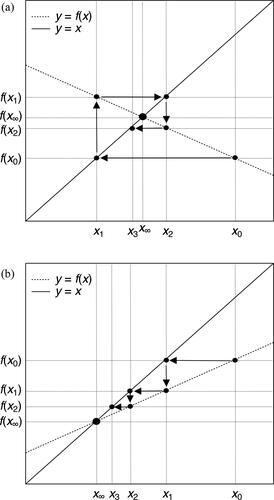
It can be seen that a convergent solution requires that |f ′(x)| < 1, or else successive points will be farther from the solution. Additionally, successive iterations (i.e. values x_i) are alternately above and below the solution for f ′(x) < 0, whereas convergence is monotonic for f ′(x) > 0. Optimal convergence occurs when f ′(x) = 0, when any initial value (sufficiently close to the solution that linearized analysis accurately captures the convergence behavior) will, upon the first iteration, yield the actual solution – that is, the horizontal line through (x₀, f(x₀)) intersections the line y = x at the solution x_∞.

Application of optimal iteration to Equation (2)(2) $$\frac{d_{\text{mob}}}{C\left(d_{\text{mob}}\right)}=X,$$(2) yields a general expression for the iteration scheme, d_mob,i+1 = Xⁿ⋅[C(d_mob,i)]ⁿ/d_mob,i^n-1, which encompasses the three specific ones discussed above: n = 1 in Equation (3)(3) $$d_{\text{mob},i+1}=X\cdot C\left(d_{\text{mob},i}\right).$$(3) , n = 1/2 in Equation (4)(4) $$d_{\text{mob},i+1}={\left[d_{\text{mob},i}\cdot X\cdot C\left(d_{\text{mob},i}\right)\right]}^{\frac{1}{2}}.$$(4) , and n = 2/3 in Equation (5)(5) $$d_{\text{mob},i+1}={\left\{d_{\text{mob},i}\cdot X^2\cdot {\left[C\left(d_{\text{mob},i}\right)\right]}^2\right\}}^{\frac{1}{3}}.$$(5) . The convergence properties of the various schemes are determined by R_ε, which is equal to (10) $$R_{\epsilon }=n\cdot \frac{d\mathit{ln}C}{d\mathit{ln}{d}_{\text{mob}}}-\left(n-1\right)=1-n\cdot \left(1-\frac{d\mathit{ln}C}{d\mathit{ln}{d}_{\text{mob}}}\right).$$(10)

As the quantity in parentheses in the last term on the right-hand side decreases from near 2 to near 1 as mobility diameter increases from low values to high values, R_ε ranges from near 1 - 2n for low mobility diameters to near 1 - n for large mobility diameters. The choice n = 1, Equation (3)(3) $$d_{\text{mob},i+1}=X\cdot C\left(d_{\text{mob},i}\right).$$(3) , provides the optimal scheme for large mobility diameters, for which dlnC/dlnd_mob is near 0. The choice n = 1/2, Equation (4)(4) $$d_{\text{mob},i+1}={\left[d_{\text{mob},i}\cdot X\cdot C\left(d_{\text{mob},i}\right)\right]}^{\frac{1}{2}}.$$(4) , provides the optimal scheme for low mobility diameters, for which dlnC/dlnd_mob is near −1. The optimal scheme covering the entire range of mobility diameters considered results from the choice n = 2/3, Equation (5)(5) $$d_{\text{mob},i+1}={\left\{d_{\text{mob},i}\cdot X^2\cdot {\left[C\left(d_{\text{mob},i}\right)\right]}^2\right\}}^{\frac{1}{3}}.$$(5) , which follows from the analysis resulting in Equation (19)(19) $${\mathit{Re}}_{i+1}={\left\{\frac{Y^2}{{\mathit{Re}}_i\cdot {\left[C_D\left({\mathit{Re}}_i\right)\right]}^2}\right\}}^{\frac{1}{3}}.$$(19) , as the limiting values of dlnC/dlnd_mob are −1 and 0. For this choice, R_ε ranges between −1/3 and +1/3, yielding rapid convergence over the entire range of particle sizes. As R_ε never exceeds 1/3 in magnitude, the fractional error decreases by more than an order of magnitude every two iterations.

Selection of initial value for the mobility diameter

Every iteration scheme requires an initial value (i.e. starting guess), and obviously the closer this value is to the actual solution, the fewer iterations will be required to attain a given accuracy. One approach that often works to find a good initial value is to merge the asymptotic solutions for small and large values of the independent variable. For determination of the mobility diameter for Equation (3)(3) $$d_{\text{mob},i+1}=X\cdot C\left(d_{\text{mob},i}\right).$$(3) , d_mob ≈ (2aλX)^1/2, with a near 1.65, for small mobility diameters, and d_mob ≈ X for large mobility diameters. One way to merge these two solutions is to take their sum: d_mob,0 = (2aλX)^1/2 + X. This provides a rather crude starting guess, overestimating the actual value by up to 35%, although the rapid convergence of the optimal iteration scheme determined above ensures that the fractional error will be less than 0.5% within three iterations for any value of d_mob. A better merger for this example is the square root of the sum of the squares of the asymptotic values: d_mob,0 = (2aλX + X²)^1/2. This underestimates the actual value by no more than 6% (and thus is better than the initial value proposed by Mulholland et al. (2006), which underestimates the actual solution by up to 16%), ensuring that the actual solution will be approached within 1% after only two iterations. In fact, this combination of starting guess and the optimal iterative scheme with n = 2/3 provides even faster convergence, with maximum fractional uncertainty no more than 1.05% after a single iteration. The reason for this rapid convergence is that the accuracy of the initial guess is highest where convergence is slowest, and vice-versa; the initial value is very accurate at both low and high mobility diameters, where R_ε is near 1/3 in magnitude, and has the largest uncertainties at intermediate mobility diameters, where R_ε is near zero.

Example 2: Calculation of aerodynamic diameter

The next example to which optimal iteration will be applied is the calculation of the aerodynamic diameter, d_aero, of a particle with density ρ and diameter d. This quantity is defined as the diameter of a particle with density ρ₀ = 1 g cm⁻³ that has the same Stokes’ settling velocity as the given particle (Brockmann and Rader 1990; DeCarlo et al. 2004), and thus satisfies the equation ρ₀⋅d_aero²⋅C(d_aero) = ρ⋅d²⋅C(d), which is obtained by matching the aerodynamic drag force to the gravitational or centripetal force (actually, any force that is directly proportional to the mass of the particle). Following the same approach that was employed to determine the mobility diameter, this equation can be written in the form (11) $${d_{\text{aero}}}^2\cdot C\left(d_{\mathrm{aero}}\right)=Y,$$(11) where Y ≡ (ρ/ρ₀)⋅d²⋅C(d) is independent of d_aero. Most of the literature that deals with this equation does not discuss how it is to be solved, one exception being Raabe (1976), who stated that the solution “must be calculated by iteration,” but gave no further details.

One iteration scheme that can be applied to Equation (11) is (12) $$d_{\text{aero},i+1}={\left[\frac{Y}{C\left(d_{\text{aero},i}\right)}\right]}^{\frac{1}{2}}.$$(12)

The results of this scheme are shown for d_aero from 1 to 1000 nm in Figure 5 as the percent difference of successive iterations from the actual value, with an initial value of 50% greater than the solution to better illustrate the convergence properties. This scheme converges rapidly for large aerodynamic diameters, with successive iterations for aerodynamic diameter 500 nm, with initial value 750 nm, given by 521, 503, 500.3, and 500.04 nm, but converges slower for small aerodynamic diameters, with successive iterations for aerodynamic diameter 5 nm, with initial value 7.5 nm, yielding 6.1, 5.5, 5.2, and 5.1 nm (Figure 5).

Figure 5. Percent differences from actual values of aerodynamic diameter, d_aero, of the successive iterations using schemes given by Equation (12)(12) $$d_{\text{aero},i+1}={\left[\frac{Y}{C\left(d_{\text{aero},i}\right)}\right]}^{\frac{1}{2}}.$$(12) , black; Equation (13)(13) $$d_{\text{aero},i+1}=\frac{Y}{d_{\text{aero},i}\cdot C\left(d_{\text{aero},i}\right)}$$(13) , red; and Equation (14)(14) $$d_{\text{aero},i+1}=\frac{Y^n}{{d_{\text{aero},i}}^{2n-1}\cdot C^n\left(d_{\text{aero},i}\right)};.$$(14) with n = 2/3, blue, as a function of aerodynamic diameter.

An alternative iterative scheme given by (13) $$d_{\text{aero},i+1}=\frac{Y}{d_{\text{aero},i}\cdot C\left(d_{\text{aero},i}\right)}$$(13) has very rapid convergence for small aerodynamic diameters, but very slow convergence for large aerodynamic diameters (Figure 5). For example, successive iterations for aerodynamic diameter 5 nm, with initial value 7.5 nm, yield 4.97 and 5.0004 nm, whereas those for aerodynamic diameter 500 nm, with initial value 750 nm, are 363, 629, 418, and 570 nm.

To apply optimal iteration to Equation (11), both sides are raised to a yet to be determined power n, and the result is solved for d_aero: (14) $$d_{\text{aero},i+1}=\frac{Y^n}{{d_{\text{aero},i}}^{2n-1}\cdot C^n\left(d_{\text{aero},i}\right)};.$$(14)

For n = 1/2 this is Equation (12)(12) $$d_{\text{aero},i+1}={\left[\frac{Y}{C\left(d_{\text{aero},i}\right)}\right]}^{\frac{1}{2}}.$$(12) , and for n = 1 this is Equation (13)(13) $$d_{\text{aero},i+1}=\frac{Y}{d_{\text{aero},i}\cdot C\left(d_{\text{aero},i}\right)}$$(13) . The convergence ratio corresponding to Equation (14)(14) $$d_{\text{aero},i+1}=\frac{Y^n}{{d_{\text{aero},i}}^{2n-1}\cdot C^n\left(d_{\text{aero},i}\right)};.$$(14) follows from Equation (6)(6) $$R_{\epsilon }\equiv \underset{i\to \infty }{\lim }\frac{{\epsilon }_{i+1}}{{\epsilon }_i}={\left[\left(\frac{x}{f}\right)\cdot \left(\frac{df}{dx}\right)\right]|}_{x_{\infty }}={\frac{d\hspace{0.17em}\text{ln}\hspace{0.17em}f}{d\hspace{0.17em}\text{ln}\hspace{0.17em}x}|}_{x_{\infty }}$$(6) : (15) $$R_{\epsilon }=-\left(2n-1\right)-n\cdot \frac{d\mathit{ln}C}{d\mathit{ln}{d}_{\text{aero}}}=1-n\cdot \left(2+\frac{d\mathit{ln}C}{d\mathit{ln}{d}_{\text{aero}}}\right),$$(15) which ranges from near 1 - n for small aerodynamic diameters to near 1 - 2n for large aerodynamic diameters. For the iteration scheme given by Equation (12)(12) $$d_{\text{aero},i+1}={\left[\frac{Y}{C\left(d_{\text{aero},i}\right)}\right]}^{\frac{1}{2}}.$$(12) , for which n = 1/2, R_ε = (-1/2)⋅dlnC/dlnd_aero and ranges from near 0.5 for small aerodynamic diameters, implying rather slow convergence, to near zero for large aerodynamic diameters, implying quite rapid convergence (Figure 5). 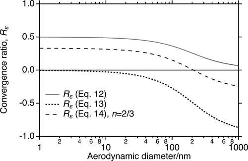Conversely, for the iteration scheme given by Equation (13)(13) $$d_{\text{aero},i+1}=\frac{Y}{d_{\text{aero},i}\cdot C\left(d_{\text{aero},i}\right)}$$(13) , for which n = 1, R_ε = -(1 + dlnC/dlnd_aero), which ranges from near 0 for small aerodynamic diameters, implying very rapid convergence, to near −1 for large aerodynamic diameters, implying quite slow convergence (Figure 6). An optimal iterative scheme that yields rapid convergence over the entire range of d_aero is given by the choice n = 2/3, for which R_ε ranges between +1/3 and −1/3 (Figure 6), implying a decrease in the fractional uncertainty of at least an order of magnitude for each two iterations. The results of this iteration scheme are also shown in Figure 5.

Figure 6. Convergence ratio, R_ε, given by Equation (15)(15) $$R_{\epsilon }=-\left(2n-1\right)-n\cdot \frac{d\mathit{ln}C}{d\mathit{ln}{d}_{\text{aero}}}=1-n\cdot \left(2+\frac{d\mathit{ln}C}{d\mathit{ln}{d}_{\text{aero}}}\right),$$(15) evaluated for the iteration schemes given by Equations (12)–(13), and Equation (14)(14) $$d_{\text{aero},i+1}=\frac{Y^n}{{d_{\text{aero},i}}^{2n-1}\cdot C^n\left(d_{\text{aero},i}\right)};.$$(14) with n = 2/3, as functions of the aerodynamic diameter.

An accurate initial value for d_aero as a function of Y for Equation (11) will minimize the number of iterations required to attain a given accuracy. For low values of d_aero, for which C is approximately equal to 2aλ/d_aero, d_aero ≈ Y/(2aλ), whereas for large aerodynamic diameters, for which C is near unity, d_aero ≈ Y^1/2. The harmonic sum (the reciprocal of the sum of the reciprocals) of these two asymptotic values, d_aero,o = 1/{[1/(Y/(2aλ)] + 1/(Y^1/2)}, understimates the actual solution by up to nearly 30%, but the expression d_aero,o = 1/{[1/(Y/(2aλ)]² + 1/(Y^1/2)²}^1/2 overstimates the actual values by no more than ∼7%. Using this latter expression as the initial value for the optimal iterative scheme given by Equation (14)(14) $$d_{\text{aero},i+1}=\frac{Y^n}{{d_{\text{aero},i}}^{2n-1}\cdot C^n\left(d_{\text{aero},i}\right)};.$$(14) with n = 2/3, for which the magnitude of R_ε never exceeds 1/3, will thus yield values that are within 1% of the true value within two iterations. However, as with the situation above for mobility diameter, the convergence is even more rapid because R_ε is lowest where the initial value is least accurate and vice-versa. As a result, the first iteration is accurate to within 1.3% and the second to within 0.3% over the entire range of d_aero.

Relation between diameter and terminal velocity of a large sphere

With increasing particle diameter, the Cunningham correction becomes progressively closer to unity and thus less important, decreasing from ∼1.15 for d_mob = 1 µm to less than 1.01 for d_mob = 20 µm, above which it can be taken as unity with little loss in accuracy. However, other effects concurrently become important and Stokes’ Law increasingly underestimates the aerodynamic drag force on a particle due to nonlinearities in the motion of the surrounding fluid, and hence overestimates the terminal velocity, u. For particles with diameter 20 µm, this overestimation is only ∼1%, but it increases to more than 5% at diameter 50 µm, 20% at 100 µm, and a factor of 2 at 250 µm.

The motion of a spherical particle in this size range is best treated in terms of two dimensionless numbers: the Reynolds number, Re ≡ du/ν_g, where ν_g is the kinematic viscosity of the gas in which the particle is moving (assumed to be air), and the drag coefficient, C_D, a normalized force, defined by (16) $$C_D\equiv \frac{F_{\text{aero}}}{\left(\frac{{\rho }_g{u}^2}{2}\right)\cdot \left(\frac{\pi d^2}{4}\right)}=\left(\frac{4}{3}\right)\cdot \left(\frac{{\rho }_p}{{\rho }_g}\right)\cdot \left(\frac{gd}{u^2}\right),$$(16) where ρ_g is the density of the gas, ρ_p is the density of the particle, and g is the acceleration due to gravity. The second equality in Equation (16)(16) $$C_D\equiv \frac{F_{\text{aero}}}{\left(\frac{{\rho }_g{u}^2}{2}\right)\cdot \left(\frac{\pi d^2}{4}\right)}=\left(\frac{4}{3}\right)\cdot \left(\frac{{\rho }_p}{{\rho }_g}\right)\cdot \left(\frac{gd}{u^2}\right),$$(16) holds because at terminal velocity the aerodynamic drag force is equal to the gravitational force. The dependences of the density and viscosity of the gas on temperature and pressure make treatment of this problem much more straightforward in terms of the dimensionless quantities Re and C_D than in terms of d and u. For the examples considered here, a particle density of 10³ kg m⁻³ is assumed, and the temperature and pressure are taken as 20 °C and 1 atm, respectively, at which the kinematic viscosity of air is 1.51⋅10⁻⁵ m² s⁻¹ and the density of air is 1.20 kg m⁻³. Reynolds numbers from 0.002 up to 4000 are considered, corresponding to diameters 10 µm to 5 mm and terminal velocities 0.3 cm s⁻¹ to nearly 12 m s⁻¹.

For a rigid sphere, C_D is a function of only Re (Rayleigh 1909-1910). Water drops with diameters up to near 1 mm falling at their terminal velocities behave like rigid spheres (Pruppacher and Beard 1970), and thus this analysis applies also to them. A multitude of relations for C_D(Re) have been proposed, but here the expression of Brown and Lawler (2003) will be used (Figure 7); many others are very similar, and the differences are small and inconsequential for the purposes of illustrating the technique of optimal iteration. For small Re, C_D ≈ 24/Re (Figure 7), which is Stokes’ Law, and the aerodynamic drag force is directly proportional to both the speed and the particle diameter. In this limit, u ≈ (1/18)⋅(ρ_p/ρ_g)⋅(g/ν_g)⋅d² and d ≈ [18⋅(ρ_g/ρ_p)⋅(ν_g²/g)⋅Re]^1/3. With increasing Re over the range considered, C_D decreases continuously to near a nearly constant value C_D,∞ ≈ 0.39 (Figure 7). For constant C_D, the aerodynamic drag force is directly proportional to the square of the speed and the square of the particle diameter. In this limit, u ≈ [(4/3)⋅(ρ_p/ρ_g)⋅(g/C_D,∞)⋅d]^1/2 and d ≈ [(3/4)⋅(ρ_g/ρ_p)⋅(ν_g²/g)⋅C_D,∞⋅Re²]^1/3. The quantity that will be important in determining the convergence rates of various iteration schemes discussed below is dlnC_D/dlnRe, which ranges from −1 for low Re to near zero for large Re (Figure 8).

Figure 7. Drag coefficient, C_D, with asymptotic limits for small and large Reynolds number, Re, and quantities Re²⋅C_D and Re/C_D, as functions of Re.

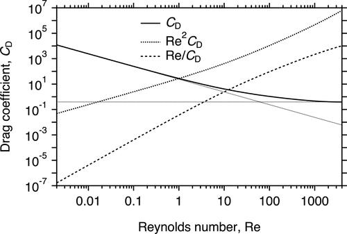
Figure 8. Logarithmic derivative of drag coefficient, C_D, with respect to Reynolds number, Re, and convergence ratio, R_ε, for Equations (19)(19) $${\mathit{Re}}_{i+1}={\left\{\frac{Y^2}{{\mathit{Re}}_i\cdot {\left[C_D\left({\mathit{Re}}_i\right)\right]}^2}\right\}}^{\frac{1}{3}}.$$(19) and (20)(20) $${\mathit{Re}}_{i+1}={\left\{{\mathit{Re}}_i\cdot X^2\cdot {\left[C_D\left({\mathit{Re}}_i\right)\right]}^2\right\}}^{\frac{1}{3}}.$$(20) , as functions of Re.

Determination of the terminal velocity for a given particle diameter, or the diameter of a particle with given terminal velocity, is not straightforward because of the nonlinear relation between C_D and Re. Although the literature is rife with relations between d and u, and graphical approaches and look-up tables have also been proposed, only iteration will be examined here, and only the optimal schemes will be presented. Two relations that will prove useful for relating diameter and terminal velocity are (17) $${\mathit{Re}}^2\cdot C_D(Re)=(\frac{4}{3})(\frac{{\rho }_p}{{\rho }_g})(\frac{d^{3}g}{{{\nu }_g}^2}){(\frac{d}{d^{\mathrm{*}}})}^3\equiv Y,$$(17) where $d^{\mathrm{*}}\equiv {\left[\left(\frac{3}{4}\right)\cdot \left(\frac{{\rho }_g}{{\rho }_p}\right)\cdot \left(\frac{{{\nu }_g}^2}{g}\right)\right]}^{\frac{1}{3}}$ is approximately 28 µm, and (18) $$\frac{Re}{C_D\left(Re\right)}=\left(\frac{3}{4}\right)\cdot \left(\frac{{\rho }_g}{{\rho }_p}\right)\cdot \left(\frac{u^3}{{\nu }_{g}g}\right)\equiv {\left(\frac{u}{u^{\mathrm{*}}}\right)}^3\equiv X,$$(18) where $u^{\mathrm{*}}\equiv {\left[\left(\frac{4}{3}\right)\cdot \left(\frac{{\rho }_p}{{\rho }_g}\right)\cdot \left({\nu }_{g}g\right)\right]}^{\frac{1}{3}}$ is approximately 0.55 m s⁻¹. Both Y and X are shown in Figure 7 as a function of Re. From Equations (17)(17) $${\mathit{Re}}^2\cdot C_D(Re)=(\frac{4}{3})(\frac{{\rho }_p}{{\rho }_g})(\frac{d^{3}g}{{{\nu }_g}^2}){(\frac{d}{d^{\mathrm{*}}})}^3\equiv Y,$$(17) and (18)(18) $$\frac{Re}{C_D\left(Re\right)}=\left(\frac{3}{4}\right)\cdot \left(\frac{{\rho }_g}{{\rho }_p}\right)\cdot \left(\frac{u^3}{{\nu }_{g}g}\right)\equiv {\left(\frac{u}{u^{\mathrm{*}}}\right)}^3\equiv X,$$(18) , iterations schemes for determination of u from a known value of d, and of d from a known value of u, can be obtained from a corresponding determination of Re from a known value of either Re²⋅C_D or Re/C_D.

The terminal velocity for a given diameter can be determined from the value of Re that satisfies Equation (17)(17) $${\mathit{Re}}^2\cdot C_D(Re)=(\frac{4}{3})(\frac{{\rho }_p}{{\rho }_g})(\frac{d^{3}g}{{{\nu }_g}^2}){(\frac{d}{d^{\mathrm{*}}})}^3\equiv Y,$$(17) . This equation is (coincidently) very similar to Equation (11), with d_aero replaced by Re, C(d_aero) replaced by C_D, and Y equal to the known quantity on the right-hand side (the similarity of the names for the quantities C and C_D is likewise coincidental). As with Equation (11), there are a variety of iteration schemes that can be employed, but the optimal one over the entire range of values of Re considered follows from the analysis presented after Equation (15)(15) $$R_{\epsilon }=-\left(2n-1\right)-n\cdot \frac{d\mathit{ln}C}{d\mathit{ln}{d}_{\text{aero}}}=1-n\cdot \left(2+\frac{d\mathit{ln}C}{d\mathit{ln}{d}_{\text{aero}}}\right),$$(15) , with n = 2/3: (19) $${\mathit{Re}}_{i+1}={\left\{\frac{Y^2}{{\mathit{Re}}_i\cdot {\left[C_D\left({\mathit{Re}}_i\right)\right]}^2}\right\}}^{\frac{1}{3}}.$$(19)

As with the situations for mobility and aerodynamic diameter, were only a restricted range of Re to be of interest, a different optimal iteration scheme could be found using Equation (9)(9) $$n_{\text{opt}}=\frac{1}{1-\frac{1}{2}\cdot (\frac{d\mathit{ln}f}{d\mathit{ln}x}{|}_{\text{lo}}+\frac{d\mathit{ln}f}{d\mathit{ln}x}{|}_{\text{hi}}}),$$(9) . For a given value of d, the right-hand side of Equation (17)(17) $${\mathit{Re}}^2\cdot C_D(Re)=(\frac{4}{3})(\frac{{\rho }_p}{{\rho }_g})(\frac{d^{3}g}{{{\nu }_g}^2}){(\frac{d}{d^{\mathrm{*}}})}^3\equiv Y,$$(17) determines Y, and an initial value is substituted into Equation (19)(19) $${\mathit{Re}}_{i+1}={\left\{\frac{Y^2}{{\mathit{Re}}_i\cdot {\left[C_D\left({\mathit{Re}}_i\right)\right]}^2}\right\}}^{\frac{1}{3}}.$$(19) and iterated until satisfactory convergence is attained, after which u is determined from the given d and the definition of Re.

The convergence ratio for this iteration scheme, R_ε = -(1/3)⋅(1 + 2⋅dlnC_D/dlnRe), never exceeds 1/3 in magnitude over the range of Re considered (Figure 8), and thus the fractional error in the iterated value decreases by at least an order of magnitude for each two iterations. In practice, convergence is even faster. For low Re, Equation (17)(17) $${\mathit{Re}}^2\cdot C_D(Re)=(\frac{4}{3})(\frac{{\rho }_p}{{\rho }_g})(\frac{d^{3}g}{{{\nu }_g}^2}){(\frac{d}{d^{\mathrm{*}}})}^3\equiv Y,$$(17) yields Re ≈ Y/24, and for high Re, Re ≈ (Y/C_D,∞)^1/2. Taking the harmonic sum of these two limits yields an initial value, Re₀ = 1/[1/(Y/24) + 1/(Y/C_D,∞)^1/2], that is accurate to within ∼20% over the entire range of Re considered. As with the situations above for determinations of the mobility diameter and aerodynamic diameter, the convergence ratio is largest in magnitude where the initial value is accurate, and near zero where the initial guess is most inaccurate (Figure 8). Thus, one iteration yields values that are accurate to within 1.7%, and two iterations yield values that are accurate to within 0.3%, over the entire range of Re considered.

Determination of d from a known value of u proceeds similarly using Equation (18)(18) $$\frac{Re}{C_D\left(Re\right)}=\left(\frac{3}{4}\right)\cdot \left(\frac{{\rho }_g}{{\rho }_p}\right)\cdot \left(\frac{u^3}{{\nu }_{g}g}\right)\equiv {\left(\frac{u}{u^{\mathrm{*}}}\right)}^3\equiv X,$$(18) . This equation is (coincidentally) similar in structure to Equation (2)(2) $$\frac{d_{\text{mob}}}{C\left(d_{\text{mob}}\right)}=X,$$(2) , with d_mob replaced by Re, the Cunningham correction replaced by C_D, and X equal to the known quantity on the right-hand side. The optimal iteration scheme for this equation is thus analogous to Equation (5)(5) $$d_{\text{mob},i+1}={\left\{d_{\text{mob},i}\cdot X^2\cdot {\left[C\left(d_{\text{mob},i}\right)\right]}^2\right\}}^{\frac{1}{3}}.$$(5) : (20) $${\mathit{Re}}_{i+1}={\left\{{\mathit{Re}}_i\cdot X^2\cdot {\left[C_D\left({\mathit{Re}}_i\right)\right]}^2\right\}}^{\frac{1}{3}}.$$(20)

The value of X is calculated from a known value of u from Equation (18)(18) $$\frac{Re}{C_D\left(Re\right)}=\left(\frac{3}{4}\right)\cdot \left(\frac{{\rho }_g}{{\rho }_p}\right)\cdot \left(\frac{u^3}{{\nu }_{g}g}\right)\equiv {\left(\frac{u}{u^{\mathrm{*}}}\right)}^3\equiv X,$$(18) , and an initial value of Re is iterated using Equation (20)(20) $${\mathit{Re}}_{i+1}={\left\{{\mathit{Re}}_i\cdot X^2\cdot {\left[C_D\left({\mathit{Re}}_i\right)\right]}^2\right\}}^{\frac{1}{3}}.$$(20) until sufficiently convergent, from which the value of d can be determined from the given value of u using the definition of Re.

The convergence ratio R_ε = (1/3)⋅(1 + 2⋅dlnC_D/dlnRe) is the negative of that for Equation (19)(19) $${\mathit{Re}}_{i+1}={\left\{\frac{Y^2}{{\mathit{Re}}_i\cdot {\left[C_D\left({\mathit{Re}}_i\right)\right]}^2}\right\}}^{\frac{1}{3}}.$$(19) , and thus also never exceeds 1/3 in magnitude (Figure 8). An initial value given by Re₀ = (24X)^1/2 + X⋅C_D,∞, the sum of the asymptotic solutions for low Re and for high Re, is accurate to within ∼20%, but a better choice is the square root of the sum of the squares of the asymptotic solutions: Re₀ = [24X + (X⋅C_D,∞)²]^1/2. Although it is accurate to only within ∼40%, the largest inaccuracies occur where R_ε is near zero, and thus it will yield more rapid convergence: the first iteration yields values that are accurate to within ∼4%, and the second iteration yields values that are within 0.7% of the actual value, over the entire range of Re considered.

Summary

Various iteration schemes for equations of interest to aerosol dynamics have been presented and the convergence behaviors of these schemes have been analyzed and explained. The technique of optimal iteration was introduced and a procedure for determining the iteration scheme that provides the most rapid convergence over a given interval was explained in detail, first in generality and then for the specific example of determining the mobility diameter from the measured mobility. A method for finding accurate initial values for iteration was presented that uses the limiting values for low and high values of the independent variable, each value being dominant in its respective limit. With suitable choice for an initial value, the technique of optimal iteration can provide more rapid convergence than might be expected, as inaccuracies in the initial values occur when the convergence rate is most rapid. The technique can be applied to other equations that are amenable to iterative solutions to determine the optimal iteration scheme and thus ensure the most rapid convergence of the iteration.

Acknowledgments

I thank Matt Boyer for valuable discussions and three anonymous reviewers for helpful comments.

Declaration of interest statement

There are no relevant financial or non-financial competing interests.

Supplemental Information

Descriptions of the optimal iteration schemes, including check values, for each of the four cases presented above are contained in the online supplementary information. The source code for all the calculations and graphs presented in this paper (in IGOR Pro 8) is available from the author upon request.

Additional information

Funding

This work was supported by the Scientific Focus Area (SFA) Science Plan program that is supported by the Office of Biological and Environmental Research in the Department of Energy, Office of Science, through the United States Department of Energy Contract No. DE-SC0012704 to Brookhaven National Laboratory.

References

- Allen, M. D., and O. G. Raabe. 1982. Re-evaluation of Millikan’s oil drop data for the motion of small particles. J. Aerosol Sci. 13 (6):537–47. doi:10.1016/0021-8502(82)90019-2.
- Brockmann, J. E., and D. J. Rader. 1990. APS response to nonspherical particles and experimental determination of dynamic shape factor. Aerosol Sci. Technol. 13 (2):162–72. doi:10.1080/02786829008959434.
- Brown, P. P., and D. F. Lawler. 2003. Sphere drag and settling velocity revisited. J. Environ. Eng. 129 (3):222–31. doi:10.1061/(ASCE)0733-9372(2003)129:3(222).
- Cunningham, E. 1910. On the velocity of steady fall of spherical particles through fluid medium. Proc. Roy. Soc. Lond. 83A:357–65.
- DeCarlo, P., J. Slowik, D. Worsnop, P. Davidovits, and J. Jimenez. 2004. Particle morphology and density characterization by combined mobility and aerodynamic diameter measurements. Part 1. Aerosol Sci. Tech. 38 (12):1185–205. doi:10.1080/02786826.2004.10399461.
- Kim, J. H., G. W. Mulholland, S. R. Kukuck, and D. Y. H. Pui. 2005. Slip correction measurements of certified PSL nanoparticles using a nanometer differential mobility analyzer (Nano-DMA) for Knudsen number from 0.5 to 83. J. Res. Natl. Inst. Stand. Technol. 110 (1):31–54. doi:10.6028/jres.110.005.
- Millikan, R. A. 1923. The general law of fall of a small spherical body through a gas, and its bearing upon the nature of molecular reflection from surfaces. Phys. Rev. 22 (1):1–23. doi:10.1103/PhysRev.22.1.
- Mulholland, G. W., N. P. Bryner, and C. Croarkin. 1999. Measurement of the 100 nm NIST SRM 1963 by differential mobility analysis. Aerosol Sci. Technol. 31 (1):39–55. doi:10.1080/027868299304345.
- Mulholland, G. W., M. K. Donnelly, C. R. Hagwood, S. R. Kukuck, V. A. Hackley, and D. Y. H. Pui. 2006. Measurement of 100 nm and 60 nm particle standards by differential mobility analysis. J. Res. Natl. Inst. Stand. Technol. 111 (4):257–312. doi:10.6028/jres.111.022.
- Pruppacher, H. R., and K. V. Beard. 1970. A wind tunnel investigation of the internal circulation and shape of water drops falling at terminal velocity in air. Q. J. Royal Met. Soc. 96 (408):247–56. doi:10.1002/qj.49709640807.
- Raabe, O. G. 1976. Aerosol aerodynamic size conventions for inertial sampler calibration. J. Air Poll. Control Assoc. 26 (9):856–60. doi:10.1080/00022470.1976.10470329.
- Rayleigh, L. 1909-1910. Notes on the application of the principles of dynamic similarity. Report for the Advisory Committee for Aeronautics, 38.
- Stokes, G. G. 1850. On the effect of the internal friction of fluids on the motion of pendulums. Trans. Camb. Phil. Soc. 9:1–99.
- Stolzenburg, M. R., and P. H. McMurry. 2008. Equations governing single and tandem DMA configurations and a new lognormal approximation to the transfer function. Aerosol Sci. Technol. 42 (6):421–32. doi:10.1080/02786820802157823.