On the variation of fricative airflow dynamics with vocal tract geometry and speech loudness

Abstract

Recent studies have determined that the number of respiratory droplets expelled during a short duration of speech can be comparable to that of a cough. Although speaking is typically modeled as a horizontal jet, recent experimental work has shown that there are large angular variations when fricative sounds are produced. To investigate this, two-dimensional vocal tract geometries for a labiodental fricative, [f] and a dental fricative, $[\theta ]$ were constructed based on magnetic resonance imaging (MRI) during these intonations. Two-dimensional ANSYS-Fluent simulations were performed to investigate the expiratory airflow from the geometries, which showed chaotic unsteady airflow trajectories with maximum velocities ranging from 20 to 40 m/s and jet trajectory angles varying between $\pm {60}^{°}.$ The simulations highlight the variabilities of the expirated airflow trajectories as a function of the type of utterance, speech loudness, size of the mouth opening, and tongue shape.

Copyright © 2022 American Association for Aerosol Research

Graphical Abstract

EDITOR:

• Yannis Drossinos

1. Introduction

During human expiratory activities such as breathing, talking, singing, laughing, coughing, or sneezing, particles are generated in the respiratory system and transported into the surroundings by the expelled airflow (Morawska et al. 2009; Gupta, Lin, and Chen 2010; Gralton et al. 2011; Bourouiba 2020). In general, larger droplets follow a ballistic-like motion such that their trajectory is not readily influenced by the velocity field, and they settle to the ground in the near-field area; usually within 1 m of the source (Gralton et al. 2011). On the other hand, smaller droplets generally follow the small-scale structures of the airflow field, due to their small Stokes number, and may remain suspended in the air for a long duration of time. These are commonly referred to as aerosols. The rate of deposition of these smaller droplets on surfaces is low as some of them can remain suspended in the air up to 30 h (Duguid 1946). However, this increases their potential to be inhaled by a susceptible person at distances greater than 1 m from the source (Morawska et al. 2020). Ambient humidity can play a critical role as evaporation can reduce droplet sizes to approximately half of their initial diameter, while only nonvolatile material remains (Nicas, Nazaroff, and Hubbard 2005). Although airborne transmission was not considered a primary route of respiratory virus transmission at the onset of the COVID-19 pandemic, the World Health Organization (WHO) now recognizes the significance of its role (WHO 2020).

Historically, greater attention has been given to violent expiratory events such as coughing and sneezing as the primary sources of respiratory particle generation (Lindsley et al. 2012; Bourouiba, Dehandschoewercker, and Bush 2014). Recent work has determined that human speech produces droplet size distributions similar to coughing and singing. While one cough can produce as many as 5,000 particles (Duguid 1945), phonation has been shown to generate between 40 to 2,600 particles per second (Asadi et al. 2020; Stadnytskyi et al. 2020), indicating that the number of particles generating by phonation and coughing may be comparable (Cole and Cook 1998).

Voiced speech is produced as lung pressure drives airflow through the vocal folds, which are located in the larynx, inciting self-sustained oscillations. The resultant unsteady modulation of the flow creates an oscillatory pressure field that acts as an acoustic source. Different sounds are produced by altering the vocal tract shape, thereby changing the resonances. Unvoiced speech sounds, classified as such because the vocal folds do not oscillate, are produced due to purely aerodynamic sound sources within the vocal tract. For example, fricatives are consonant sounds that are produced by passing air through a partial restriction in the vocal tract made by placing two articulators close together (Stevens 1999), as occurs during the pronunciation of [f]; a labiodental fricative whose constriction is generated as the lower lip is located against the upper teeth. Similarly, $[\theta ]$ is a dental fricative generated by locating the tip of the tongue against the upper teeth (Isshiki and Ringel 1964). With respect to speech as a modality for transport of infectious disease, fricatives are of interest because, during pronunciation, the constrictions created at the mouth result in increased airflow velocities (Yoshinaga, Nozaki, and Wada 2019b; Pont et al. 2019).

Understanding the size distribution and the penetration distance of respiratory droplets emitted during speech is critical for determining the risk of virus transmission. The majority of respiratory droplets expelled during speech are small, with an average diameter of 1-2 μm (Morawska et al. 2009; Somsen et al. 2020). As mentioned previously, these smaller droplets are more likely to follow the fluid streamlines than larger droplets due to their reduced Stokes numbers (Hinds 1999). However, much remains unknown about the behavior of the airflow emitted during speech.

Prior investigations have revealed that the pattern of expiratory flow is a function of utterance. Namely, Geoghegan et al. (2012) used stereo particle image velocimetry (SPIV) to quantify the airflow of two simplified in-vitro models of [s] and $[\int ]$ fricatives. They reported that the exit trajectories of [s] were primarily horizontal, while $[\int ]$ was oriented down toward the ground. Abkarian et al. (2020) measured the speech induced fluid dynamics as a function of utterance type from a single subject using correlation image velocimetry. They observed that a mix of fricative and plosive airflow trajectories produce variable ejection angles that span from -${40}^{°}$ to +${40}^{°}$ about the horizontal. For utterances produced by sequential plosive sentences, like “Peter Piper picked a peck,” the flow was more horizontal and resembled a sequence of puff flows. They then performed numerical simulations of a jet with a time-varying volumetric flow rate to understand the jet expansion associated with speaking and breathing.

Prior work has also identified how intersubject variability can result in significant variations in the expirated flow field. In-vivo investigations involving 17 males and 9 females producing a single utterance revealed velocity magnitudes were twice as high in males as in females, and that the range of velocity vector angles of the flow exiting the mouth were almost twice as high for females ($\sim {40}^{°}$) as for males ($\sim {25}^{°}$) (Kwon et al. 2012). Yoshinaga, Nozaki, and Wada (2019a) recently explored the expiratory flow during articulation of fricatives as a function of vocal tract geometry with the goal of understanding sound production. They captured the vocal tract geometry of five subjects during articulation of sibilant fricatives [s] and $[\int ],$ and explored how geometrical differences between the vocal tracts influenced the sound production of these fricatives. Large Eddy Simulations (LES) were employed to quantify the differences in fluid velocity at the tooth gap of different subjects. In addition to intersubject vocal tract geometrical variabilities, changes in the stress of the utterance, the location of the utterance in speech, and the type of utterance preceding or following the utterance of interest, impacted the sound produced (Oller 1973).

More recently, experimental investigations by our research group using both in-vivo and static physical mouth models of consonant production have quantified the variability in the expiratory flow trajectory across a wide range of consonant productions. Both inter- and intra-consonant variability were assessed. The expiratory flow trajectory as a function of consonant utterance was observed to vary over a range of approximately -${45}^{°}$ to +${40}^{°}.$ For particular consonants, the flow was shown to be unstable due to the oral geometry at the exit of the mouth. Consequently, the expirated flow was also found to be highly sensitive to small variations in the flow conditions as well as postural changes in the oral geometry (Ahmed et al. 2021).

Prior works suggest that the general flow behavior at the mouth exit during speaking is not a simple horizontal steady jet, which is often invoked to explore such expiratory flows (Abkarian et al. 2020; Yang et al. 2020; Liu et al. 2021; Singhal et al. 2021), but it is highly transient with variable airflow jet trajectories (Ahmed et al. 2021; Han et al. 2021). The main objective of this article is to numerically confirm the experimental finding that the unsteady jet associated with fricative production experiences large amplitude oscillations in the jet exit angle at the mouth. Then, the influence of small changes to the mouth morphometry and the loudness of speech (i.e., the flow rate exiting the mouth) on the expiratory jet angle is highlighted.

To achieve these objectives, a real-time magnetic resonance imaging (MRI) multimodal speech dataset (Narayanan et al. 2014) acquired at the mid-sagittal plane of speakers was used to produce a two-dimensional geometry of the vocal tract during the production of fricative consonants [f] and $[\theta ]$ to perform two-dimensional numerical simulations. The fricatives were selected based on prior work (Abkarian et al. 2020; Ahmed et al. 2021) that showed that fricatives cause large amplitude oscillations in the flow direction. In addition, these fricatives are of interest because the high airflow velocities produced by the narrow constrictions of a fricative could increase the distance the droplets travel before falling to the ground. It is acknowledged that two-dimensional simulations used in this investigation may not be exact representations of the actual three-dimensional flow fields (Anderson, Green, and Fels 2009). Nevertheless, two-dimensional simulations can provide useful insights related to variability in the expiratory jet direction, particularly with regards to sensitivity of the flow to mouth morphometry and flow rate, and the subsequent influence on the flow patterns of the expired airflow (Fu, Uddin, and Curley 2016; Bianchini et al. 2017).

The vocal tract geometry, the numerical model, and the computational grid are discussed in detail in Section 2. The accuracy of the numerical procedure is verified by comparing the results with experimental particle image velocimetry (PIV) data in Section 3.1. By exploring the numerical results for [f] and $[\theta ]$ utterances, the general characteristics of the airflow during the production of fricatives and the influence of utterance are identified in Section 3.2. Then, the effects of tooth gap (Section 3.3), loudness (Section 3.4), and tongue shape (Section 3.5) on the expelled airflow are explored. Additionally, the propagation distance of the expirated flow field is investigated in Section 3.6. Finally, the conclusions are discussed in Section 4.

2. Methods

2.1. Vocal tract geometry

Due to the high variability in oral geometry from subject to subject, a generalized geometry was developed based on MRI acquisitions of speakers producing fricative consonants, as contained in the USC-TIMIT database (Narayanan et al. 2014). Figure 1a shows the resultant generalized geometry overlaid on the MRI of a male subject when the lower lip is located adjacent to the upper incisors to generate a labiodental constriction as occurs when pronouncing the utterance [f]. Although the generalized representation is not an exact match, by design, it captures the primary features observed during this utterance. Preliminary investigations showed that the position of the tooth gap constriction and the lips’ shape significantly affect the behavior of the expiratory flow. For this reason, emphasis was placed on ensuring there was reasonable agreement between these features in the proposed geometry and the MRI data. The inset shown in Figure 1a is a zoomed-in view of the constriction geometry where h represents the tooth gap, wall-normal gap between the lower palate and the upper tooth. The geometry shown in Figure 1a is, henceforth, referred to as flat-[f].

Figure 1. Silhouette of the mouth geometries for (a) flat-[f], (b) curved-[f], and (c) flat-$[\theta ]$ models. The inset in (a) shows a zoomed-in view of the mouth geometry, with the tooth gap defined as h. Subfigures (a) and (b) are based on Figure 1 of a conference article (Mofakham et al. 2021).

As discussed in the introduction section, intersubject and intrasubject variabilities lead to vocal tract geometrical variations during speech. Accordingly, an additional model with the geometry shown in Figure 1b was also generated to explore the effects of vocal tract geometrical variations. As seen in the figure, the tongue of this model has increased curvature at its tip, and the tooth is positioned at a location where there is a steep upward slope compared to that of the flat-[f] model. The geometry shown in Figure 1b is henceforth referred to as curved-[f].

In addition, a mouth geometry representative of the utterance $[\theta ]$ was also produced from MRI geometry and is shown in Figure 1c. The two-dimensional geometry of the $[\theta ]$ model is similar to the geometry of the flat-[f] model, but with the tongue tip positioned between the lower lip and the upper tooth, generating a dental constriction. This leads to an increased distance between the lips, and different curvature along the lower boundary at the mouth exit. This geometry is referred to as flat-$[\theta ]$ in the investigations.

For $[\theta ]$ and curved-[f], the tongue covers the lower incisors, so these were not included in the $[\theta ]$ and curved-[f] models. For flat-[f], it is less clear whether the incisors should be included, but since no data was available to create a model, they were not included in the flat-[f] model either. While admittedly a simplification, the lower incisors do not influence the geometry of the minimum flow constriction and so they are not expected to have a predominant influence on the flow.

Average constriction areas of approximately $0.20{\text{cm}}^2$ have been reported for fricatives [f] and $[\theta ]$ (Narayanan, Alwan, and Haker 1995). Assuming the width of the mouth (w) is 2.5 cm, a minimum tooth gap height (h) of 0.8 mm was adopted for the two-dimensional models of [f] and $[\theta ]$ (see the inset of Figure 1a). To explore the influence of the gap height on the airflow propagation models, with a minimum gap height of 0.6, 1.0, and 1.2 mm, as listed in Table 1, were also simulated.

Table 1. Configuration of all the studied cases.

Model	Gap height (mm)	Glottal pressure (Pa)	Flow rate (L/min)
flat-[f]	0.6	300	18.00
		600	25.34
		860	30.45
flat-[f]	0.8	300	23.10
		600	33.00
		860	40.05
flat-[f]	1.0	300	30.00
		600	42.90
		860	52.95
flat-[f]	1.2	300	37.35
		600	52.80
		860	61.80
flat-$[\theta ]$	0.8	300	24.18
		600	34.40
		860	41.11
curved-[f]	0.8	300	23.55
		600	33.45
		860	40.43

The vocal tract width in the z-direction (w) is assumed to be 2.5 cm for evaluating the flow rate.

2.2. Numerical procedure

2.2.1. Numerical model

The maximum Reynolds number ($Re={\overline{V}}_{\mathit{mag}}h/\nu$) in air (ν = $1.46\times {10}^{-5}{\mathrm{m}}^2/\mathrm{s}$) was computed based on the mean velocity through the tooth gap (${\overline{V}}_{\mathit{mag}}$), and the height of the tooth gap (h). It varied from 800 to 2,900 over the range of flow and geometry parameters that were investigated. The flow field exiting the mouth cavity during fricative utterances was evaluated by direct numerical simulation of the full 2 D Navier-Stokes and continuity equations (with no need to use a turbulence model) through the commercially available ANSYS-Fluent computational fluid dynamics (CFD) software. The SIMPLE (Semi Implicit Method for Pressure Linked Equations) scheme (Patankar 2018) was implemented as the pressure velocity coupling algorithm. The least-square cell-based method was used to evaluate the gradient terms, and the second-order upwind scheme was employed to discretize the convection terms of the momentum equations. The simulations were run for a duration of 0.2 s starting from an initial quiescent state, which was selected based on the mean fricative duration reported in the literature (Oller 1973; Lass 2012). The time step of the simulations was set to ${10}^{-5}\mathrm{s}$ and a residual criterion of ${10}^{-4}$ was picked for the continuity as well as the x, and y components of the momentum equations.

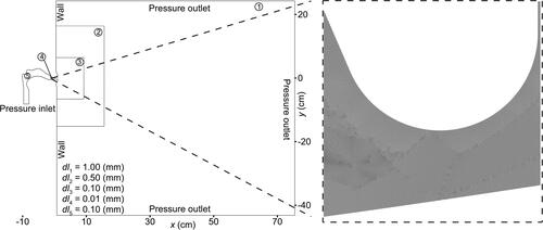
During phonation, the pressure generated in the lungs drives airflow through the vocal tract with increased pressure increasing the flow rate. The loudness of speech is also directly correlated with increased lung pressure (Titze 1984). Therefore, increasing loudness is associated with increasing the airflow rate through the vocal tract and out of the mouth. Accordingly, various constant pressures were imposed at the computational domain inlet (see Figure 2) located below the glottis (the opening between the vocal folds) to investigate soft (300 Pa), normal (600 Pa), and loud speech (860 Pa). The inlet pressure of 300 Pa results in lower volumetric flow rates compared to when the subglottal pressure is set to 600 Pa (normal speech). Similarly, the inlet pressure of 860 Pa for loud speech leads to higher volumetric flow rates than normal speech. Because atmospheric conditions are present at the exit of the mouth, a pressure outlet boundary condition with a zero gauge pressure was applied along the boundaries of the external flow domain, as shown in Figure 2. As seen in the figure, the no-slip boundary condition was applied for the vocal tract boundaries and the solid wall, which represented the speaker’s body.

Figure 2. Computational domain and the imposed boundary conditions. The regions with different grid sizes are labeled by number. The size of maximum grid size of each region is listed on the bottom right side of the figure. The inset shows the grid resolution in the tooth gap in region 4. This figure is a modified version of Figure 2 in a proceeding conference article (Mofakham et al. 2021).

The simulations of all the cases listed in Table 1 were carried out on the ACRES High-Performance Computing (HPC) cluster at Clarkson University on 20 dual Xeon gold 6230 cores.

2.2.2. Computational grids

Because the size of the domain is relatively large and there are orders of magnitude differences between the length scale at the tooth gap and the far-field area, a non-uniform grid was used based on the local length scale, as shown in Figure 2, where $d{l}_{\mathrm{n}}$ is the maximum cell size in the different regions. The inset in Figure 2 shows the grid resolution at the tooth gap in region 4. Region 4, including the narrow areas at the tooth gap and between the lip, is the most critical region of the current computational domain where the prediction of the airflow remarkably affects the general behavior of the expiratory flow. Therefore, it was essential to ensure that a refined grid was used in this region so that the boundary layers were fully captured and the resultant vortical structures were accurately resolved. Refining the grid increases the computational cost; hence, finding an optimum cell size is necessary. Accordingly, four different grids were generated for the [f] vocal tract geometry with a 0.8 mm tooth gap height, where the maximum cell size in the tooth gap area was refined as listed in Table 2, while the maximum grid size in the other regions was held constant. Simulations were performed for the different grids for 500-time steps with an inlet pressure of 600 Pa. To investigate the ability of the grids to capture the boundary layer variations in the near-wall region, the velocity profiles near the lower boundary are also presented in the inset of Figure 3. The wall-clock time per iteration and the ${\mathrm{L}}_2$ norm of the difference between the profile and the profile of the next finer mesh, normalized by the mean constriction velocity, are tabulated in Table 2.

Figure 3. Comparison of the mean velocity magnitude profiles at the tooth gap for different grid sizes.

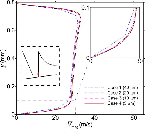
Table 2. Grid sensitivity study data.

Case	Gap max cell size (μm)	Number of cells	Wall-clock (s)	Normalized ${\mathrm{L}}_2$ norm of the differences in the velocity profiles
1	40	1,790,862	0.34	–
2	20	2,003,127	0.41	0.041
3	10	2,838,711	0.61	0.025
4	5	6,215,341	1.45	0.018

Figure 3 reveals that Cases 1 and 2, respectively, with a maximum cell size of 40 and 20 μm in the tooth gap area are not refined enough relative to the local length scale to properly capture the near-wall boundary layer, but the boundary layer was well resolved in Cases 2, 3 and 4, which indicates that a grid with a cell size equal to or smaller than 20 μm is sufficiently refined. Based on the data provided in Table 2 for CPU time, a mesh size of 10 μm was chosen as a good compromise between runtime and accuracy.

2.3. Verification process

In addition to the numerical investigations, PIV was also used to experimentally measure the airflow velocity field for a sufficient amount of time, namely 36 s (900 images acquired at 25 Hz), to acquire high fidelity measurement data at the exit of the mouth for the [f] and $[\theta ]$ geometries. The velocity measurements were acquired according to standard practices (Raffel et al. 2018) such that the uncertainty in the velocity field measurements was less than 5%. The experimental [f] geometry was fabricated by extruding the curved-[f] geometry shown in Figure 1b with a width of 2.5 cm in the spanwise direction (normal to the plane). The spanwise variations of the vocal tract geometry were ignored as the focus of this investigation was on determining the sensitivity of the flow trajectory to the mouth morphometry, which will impact both 2 D and 3 D flow simulations. In the following section, the PIV data captured from the viewing area of $74\text{mm}\times 64\text{mm}$ at the mouth exit was used for the comparison with the numerical predictions. Due to experimental restrictions, the field of view for the PIV measurements only extended from the minimum gap located at the mouth exit, as opposed to from the tooth gap. For more detailed information regarding the experimental procedure, interested readers may refer to the companion article focused on the PIV measurements (Ahmed et al. 2021).

3. Results and discussion

The 18 investigated cases are tabulated in Table 1, showing the variations in tooth gap height, subglottal pressure, and tongue shape. By exploring the fluid trajectories for different cases during [f] and $[\theta ]$ productions, the sensitivity of the flow field to geometrical variations in the oral cavity, and sound pressure level (i.e., subglottal pressure) was investigated.

3.1. Model verification

To verify the accuracy of the numerical approach used in this investigation, the data were first validated against experimental PIV velocity measurements using the curved-[f] model with a tooth gap height of 0.8 mm at a subglottal pressure of 300 Pa. The PIV velocity magnitude contours on the mid-plane time-averaged over 36 s are shown in Figure 4a, while the velocity magnitude contours predicted by the two-dimensional ANSYS-Fluent simulation time-averaged over 0.2 s are displayed in Figure 4b. Visual comparison of these figures confirms a qualitative agreement between the pattern of the jet flow predicted by the numerical approach and that of the experimental measurements, although the numerical jet is narrower and decays slower than the experimental one.

Figure 4. The mean velocity magnitude contours of (a) the PIV velocity measurements and (b) the numerical simulation of the curved-[f] model with a tooth gap height of 0.8 mm at a subglottal pressure of 300 Pa. (c) The comparison of the mean velocity magnitude profiles extracted along three lines normal to the upper lip from the experimental and numerical results, labeled in subfigures (a) and (b) as lines (1), (2), and (3).

To enable a quantitative comparison, mean velocity profiles were extracted along three lines normal to the upper lip from the experimental and numerical results, labeled in Figures 4a and b as lines (1), (2), and (3). Figure 4c plots the velocity profiles at the identified locations. The magnitude of the numerical velocity profiles along line 1 shows good agreement with the experimental measurements, but there are some discrepancies between the results at locations 2 and 3, where the numerical simulations overestimate the experimental measurements. The location of the predicted peak velocities along lines (1), (2), and (3) are also shifted slightly and are closer to the lip surface in the numerical results. In addition to the 2 D assumption of the numerical simulations, the numerical results were temporally averaged over a time span of 0.2 s, whereas the experimental data were averaged over a much longer length of time (36 s), as previously discussed. That is, the numerical simulations consider the more physiologically relevant situation that includes transient effects as the flow develops, whereas the experimental data inherently assumes the flow is at steady-state.

As will be discussed in Section 3.2, significant instability in the jet flow exists, which results in widely varying jet trajectories. While this is not as pronounced over the shorter time scale for which the numerical simulations were performed, in the experimental data, time-averaging the acquisitions over a longer time scale results in a broader jet width, with a lower peak velocity, due to the unsteadiness. This is most prominent at the two downstream locations, where the flow unsteadiness is most pronounced. In addition, the numerical simulations considered the transient flow behavior during the initiation of the flow, which decreases flow instabilities. In contrast, the experimental measurements were acquired under quasi-steady flow conditions. The challenge of detecting the wall, and resolving the near-surface flow in the experimental investigations, is another factor that may account for the discrepancies in the magnitudes and the peak locations.

3.2. Fricative consonant investigations

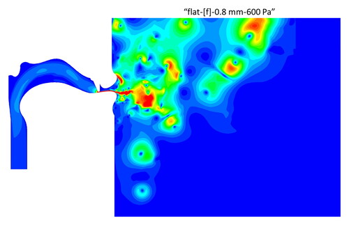
Figure 5 presents results for the flat-[f] utterance at 600 Pa with a tooth gap height of 0.8 mm. The snapshot of the instantaneous flow field at 0.1 and 0.2 s, respectively, shown in Figures 5a and b reveals a complex, vortex-laden flow field downstream of the mouth exit, and large translating vortices in the far-field flow. The vortices in the far-field area evolve over a time scale longer than the utterance time of 0.2 s, so the far-field mean flow shown in Figures 5a and b is not well established. To determine whether the near field has reached a statistical steady state, Figure 5c presents the running average of the velocity, at the middle of the tooth gap with (x, y) = (–0.84 cm, −0.25 cm), along with the instantaneous velocity at the same location. This figure confirms the time-averaged near field is reasonably converged after approximately 0.05 s.

Figure 5. (a)–(b) The instantaneous velocity magnitude $(V_{\text{mag}})$ contours of the airflow for the flat-[f] model with a tooth gap height of 0.8 mm at a subglottal pressure of 600 Pa at 0.1 and 0.2 s. (c) The time evolution of the instantaneous and mean velocity magnitude $({\overline{V}}_{\text{mag}})$ at the middle of the tooth gap during 0 to 0.2 s. (d) The corresponding jet trajectory angle evolution during 0 to 0.2 s.

The comparison of Figure 5a with Figure 5b indicates that the airflow jet exiting the mouth oscillates between the upper and lower lips. Figure 5a illustrates an upward airflow trajectory, measured relative to the horizontal, at the mouth exit, while Figure 5b shows a downward airflow trajectory. To provide more quantitative information regarding the behavior of the air jet from the mouth, the variation of the predominant jet flow direction at the mouth exit in time was evaluated. The angle (α) of a linear line, anchored to the midline of the tooth gap exit and best fit to the locations of the maximum instantaneous velocity in the range of 0 to 3 cm from the tooth, was calculated to provide the evolution of the air jet trajectory angles. The corresponding time evolution of this angle is plotted in Figure 5d, where the mean value (μ) and the standard deviation (${\sigma }_{\mathrm{N}}$) of the trajectory angle variations are also reported. Figure 5d reveals that the generated airflow trajectories oscillate with a high frequency, which was also observed in physical measurements (Ahmed et al. 2021). The airflow jet initially maintains positive fluctuating angles with a maximum angle of ${70}^{°},$ but at around 0.15 s the jet trajectory migrates toward the lower lip and becomes predominantly negative angles.

Video A in the supplementary material presents the temporal evolution of the fluid velocity magnitude through the vocal tract as it is expelled from the mouth. It should be pointed out that the red color contours in all the videos represent velocities greater than 15 m/s. The video confirms the conclusion from Figure 5d that the jet trajectory initially exhibits positive angles, which then decrease, producing a more horizontal orientation at 0.15 s.

The initial attachment of the jet to the lips occurs due to the Coanda effect (Coanda 1936), which arises from a reduction in the air pressure in the region between the jet and the adjacent lips, producing a net lateral force that moves the jet toward the adjacent surface. This is also observed in voiced speech where the jet flow exiting the glottis behaves similarly to the jet flow exiting the mouth exit (Erath and Plesniak 2006a, 2006b, 2006c).

To explore the expiratory flow during the utterance of $[\theta ],$ the flat-$[\theta ]$ model with the geometry illustrated in Figure 1c and a tooth gap height of 0.8 mm was also simulated. The corresponding contours of mean velocity magnitude at a subglottal pressure of 600 Pa and the time evolution of the jet trajectory angle are shown in Figures 6a and b, respectively. The mean velocity contours of the flat-$[\theta ]$ show that the airflow trajectories produced by the flat-$[\theta ]$ are more negative in comparison to those of the flat-[f] utterance. Figure 6b provides more detailed information by showing the time history of the jet angles. Similar to the flat-[f] model, the expirated jet initially attaches to the upper lip, producing positive jet trajectory angles before shifting toward the lower lip, resulting in negative jet angles. Despite the general similarity between the evolution pattern of the jet trajectory angle of the flat-$[\theta ]$ with that of the flat-[f] utterance, a careful comparison of Figure 6b with Figure 5d reveals distinct differences between the airflow trajectories. Namely, the shift of the jet orientation from positive angles to negative angles occurs earlier (0.09 s) for the flat-$[\theta ]$ model, when compared with the flat-[f] utterance (0.15 s). The maximum positive trajectory angle of the flat-$[\theta ]$ is ${36}^{°}$ which is approximately half of that of the flat-$[f]$ model (${70}^{°}$). In addition, the mean value of the jet trajectory angle distribution for the flat-$[\theta ]$ utterance is $-4^{°}$ which is significantly more negative than that of the flat-[f] utterance (${24.37}^{°}$). Accordingly, it is concluded that the expirated jet trajectories produced from the flat-$[\theta ]$ utterance are more likely to maintain negative angle orientations and to attach to the lower lip, which arises as a result of a larger distance between the lips and a different tongue shape for the utterance $[\theta ],$ when compared to those of the flat-[f].

Figure 6. (a) The mean velocity magnitude contours of the airflow for the flat-[$\theta$] utterance with a tooth gap height of 0.8 mm at a subglottal pressure of 600 Pa at 0.2 s. (b) The corresponding jet trajectory angle evolution during 0 to 0.2 s.

Video B in the supplementary material shows the evolution of the temporal velocity magnitude contours of the flow expelled from the flat-$[\theta ]$ model. The comparison of Video B with Video A confirms the airflow trajectories produced by the flat-$[\theta ]$ are more negative relative to those of the flat-[f] utterance.

3.3. Influence of tooth gap height

The effect of tooth gap height on the expiratory flow propagation, as might be expected to vary across speakers and for different intonations, is explored in this section. Accordingly, the mean velocity contours as well as the corresponding velocity vectors for the flat-[f] model at a subglottal pressure of 600 Pa, and different tooth gap heights of 0.6, 1.0, and 1.2 mm, were studied, and the results are illustrated in Figures 7a–c, respectively. The models with large tooth gap heights (1.0 and 1.2 mm) are more representative of aspirated configurations $[f^h].$

Figure 7. The mean velocity magnitude contours in conjunction with the superimposed mean velocity vectors of the airflow for the flat-[f] model with a tooth gap height of (a) 0.6, (b) 1.0, and (c) 1.2 mm at a subglottal pressure of 600 Pa at 0.2 s. The corresponding jet trajectory angle evolution from 0 to 0.2 s for a tooth gap height of (d) 0.6, (e) 1.0, and (f) 1.2 mm.

The orientation of the expirated jet is sensitive to the tooth gap height. As shown in the mean airflow field in Figure 7a, for the smallest tooth gap height (0.6 mm) the flow is predominantly attached to the lower lip. However, increasing the gap height to 1.0 mm (Figure 7b) results in a bifurcated mean velocity field, indicting the flow attached to both the upper and lower lip over the simulation time. Further increasing the gap height to 1.2 mm results in the jet primarily attaching to the upper lip, generating a more positive trajectory in the airflow.

The jet trajectory angle variation of the models with a tooth gap height of 0.6, 1.0, and 1.2 mm are plotted versus time in Figures 7d–f, respectively, where the mean and standard deviation of the trajectory angles are also reported. Figure 7d reveals that the jet exiting from the tooth gap height of 0.6 mm initially maintains a positive angle orientation, but shortly after (at 0.025 s) it moves toward the lower lip, generating a more negative airflow trajectory. Figure 7e shows that the expiratory jet trajectory angles during the first 0.1 s of the expiration are more positive, but then shift downward toward the lower lip, exhibiting angles that are approximately oriented about the horizontal, which produces the bimodal mean velocity field shown in Figure 7b. Figure 7f confirms that the airflow trajectories produced from the flat-[f] model with a tooth gap height of 1.2 mm are predominately oriented upward with a mean angle of ${38}^{°}.$

These findings suggest that as the tooth gap is increased, the flow trajectory becomes more positive at the mouth exit. Based on the results of the cases studied in this investigation, it is conjectured that the jet has an initial transient phase during which the jet maintains a positive angle orientation, and then it migrates toward the lower lip where it appears to stabilize and assume a straighter orientation. The duration of the initial transient phase depends on the jet velocity and the width of the jet (tooth gap height). From Figure 7 it is concluded that increasing the flow rate increases the initial transient period such that the jet maintains a positive angle longer, leading to more positive jet trajectory angles.

3.4. Influence of speech loudness

Owing to the fact that one of the objectives of this work is to characterize the influence of loudness on the flow trajectories, the flat-[f] model with a tooth gap height of 1.0 mm was investigated, as shown in Figure 8, as a function of the subglottal pressure (p_s). As seen in Figure 8a, for the smallest subglottal pressure of 300 Pa, indicative of soft speech, the jet tends to attach to the lower lip generating more negative angles and straighter airflow trajectories. Figure 8b exhibits a bimodal behavior similar to the airflow trajectories of the flat-[f] model with a tooth gap height of 1.0 mm at a normal loudness level (p_s = 600 Pa), which was already discussed in Section 3.3. Figure 8c confirms that the jet predominately attaches to the upper lip generating airflow trajectories with positive angle orientations during loud (p_s = 860 Pa) production of the [f] utterance.

Figure 8. The mean velocity magnitude contours of the airflow for the flat-[f] model with a tooth gap height of 1.0 mm at subglottal pressures of (a) 300, (b) 600, and (c) 860 Pa at 0.2 s.

To provide more information regarding the airflow trajectories generated by this model at different loudness levels, the time history and the histograms of the trajectory angle variations at subglottal pressures of 300, 600, and 860 Pa are illustrated in Figure 9, where the mean and standard deviation of the trajectory angles are also reported. Note that the vertical axis of the histogram represents the normalized number of occurrences ($N/N_{\mathrm{t}}$). The trajectory angle is computed using bins with a width of $5^{°}.$

Figure 9. The time history of jet trajectory angle for the flat-[f] model with a tooth gap height of 1.0 mm at subglottal pressures of (a) 300, (b) 600, and (c) 860 Pa from 0 to 0.2 s. The corresponding trajectory angle histogram distributions during 0 to 0.2 s at subglottal pressures of (d) 300, (e) 600, and (f) 860 Pa.

The time history of the trajectory angle for soft speech (p_s = 300 Pa) is plotted in Figure 9a. The jet initially exhibits some oscillations over a duration of ∼0.025 s, and then predominantly positive jet trajectories are produced. Shortly after ∼0.05 s the flow trajectory becomes more negatively oriented. The jet also experiences some rapid changes in its trajectory (e.g., at 0.19 s), which is a result of the interactions of the jet with the vortex structures that were expired into the surrounding area at earlier instances in time. A bimodal configuration (positive jets with an angle around ${25}^{°}$ and negative jets with an angle around $-{10}^{°}$) is observed in Figure 9d, while the overall mean trajectory angle is $2^{°}.$ The time history and histogram of the trajectory angle at a normal loudness (p_s = 600 Pa) are plotted in Figures 9b and e, respectively. The comparison of these figures with Figures 9a and d confirms a roughly comparable bimodal pattern. Nonetheless, increasing the subglottal pressure from a low level to the normal loudness level increases the duration that the jet maintains its initial upward trajectories, which results in a higher mean trajectory angle, a reduction in the number of jet occurrences with negative angles, and an increase in the number of occurrences with positive angles. The time history and the histogram of the trajectory angles generated during the loud utterance production (p_s = 860 Pa), plotted in Figure 9c and f, show almost a normal distribution with a mean angle of ${35}^{°}.$ Comparing Figure 9c with Figure 9a and b clarifies that the directions of the jet trajectories produced by this model are positive for a longer period of time than those of the low and normal loudness.

3.5. Influence of tongue shape

To quantify how small morphological changes influence the airflow trajectories, the simulation results of the curved-[f] model with a curved tongue tip illustrated in Figure 1b, are explored in this section, and the results are compared with those of the flat-[f] model with a flatter tongue tip (Figure 1a). The mean velocity magnitude contours and the velocity vectors for the curved-[f] and the flat-[f] model with a tooth gap height of 0.8 mm at a subglottal pressure of 300 Pa are shown in Figures 10a and b, respectively. The histograms of the trajectories are plotted in Figures 10c and d, respectively, as well.

Figure 10. The mean velocity magnitude contours in conjunction with the superimposed mean velocity vectors of the airflow for (a) the curved-[f] and (b) the flat-[f] models with a tooth gap height of 0.8 mm at a subglottal pressure of 300 Pa at 0.2 s. The corresponding trajectory angle histogram distributions during 0 to 0.2 s for (c) the curved-[f] and (d) the flat-[f] models.

The mean velocity magnitude contours plotted in Figure 10a are the result of predominantly positive-oriented jet trajectories produced by the curved-[f] model, while Figure 10c shows that the jet trajectories of this case have a roughly normal distribution with a mean angle of ${35}^{°}.$ Video C, which can be found in the supplementary material, presents the instantaneous velocity magnitude contours of the curved-[f] model. The video reveals that the jet predominantly attaches to the upper lip generating stationary positive angle trajectories. The mean velocity contour of the flat-[f], shown in Figure 10b, is produced by predominantly negative airflow trajectories. The histogram of the trajectory angle distributions plotted in Figure 10d confirms this. Video D, showing the instantaneous magnitude velocity contours of this case, confirms a short duration of initially positive trajectories that are subsequently followed by more horizontal and negative oriented jet trajectories (see supplementary material).

3.6. Expirated flow propagation

By exploring the results of the 18 cases listed in Table 1, the general pattern of the expiratory flow during sustained production of [f] and [θ] fricative utterances from a vocal tract with a flat and curved tongue was identified. It was found that for every case, initially positive jet trajectories are produced, but the duration of these positive jet trajectories depends on the vocal tract geometry and the flow rate. Due to the increased slope of the tongue, the curved model produced positive trajectories for the low, normal, and high loudness levels. However, for the model with a flat tongue, the probability of positively angled jet trajectories depends on the expiratory flow rate. Increasing the flow rate extends the duration of the positive trajectory productions. Roughly, the same patterns in the expiratory flow are observed during [f] and [θ] productions, but the larger distance between the lower lip and the upper lip of the [θ] utterance increases the tendency of the jet to migrate toward the lower lip and reduces the duration of the positive angle jet trajectory productions.

Based on the expiratory flow pattern recognized for different cases, the potential propagation distance and direction of airflow and respiratory droplets can be identified. As previously discussed, smaller droplets follow the flow and are spread in different directions with the oscillating jet trajectory orientations. Since the duration of predominantly positive jet trajectories increases with increasing flow rate, smaller respiratory droplets are likely to be transported into the upper regions of the flow domain for higher flow rates. This increases the chance of small droplets staying suspended in the surrounding air, and thereby, being transmitted to the far-field region by any ambient air currents. Also, it is known that the number of respiratory droplets produced during speech increases with loudness (Asadi et al. 2019), hence it is expected more respiratory droplets will also be produced, further increasing the risk of droplet transport from the near field to the far-field. On the other hand, for smaller flow rates, the expirated airflow and smaller droplets are spread in the negative and horizontally oriented directions. For the curved tongue models, positive jet angle trajectories are predominant, independent of flow rate, which is likely to result in the transport of aerosols into the upper region of the flow domain. While studies of the flow field inform how droplets are likely to be transported, virus transmission (e.g., infection risk) is much more complex.

The large airflow velocity of around 30 m/s at the constriction region (see Figure 5) reveals the high potential for large droplet propagation with ballistic motion in the near-field of the speaker. Because the passage at the constriction region of the flat tongue model is almost horizontal, the airstream at the tooth gap exit is mainly horizontal. Consequently, it is reasonable to assume that large droplets will be expelled predominantly in the horizontal direction as well. However, the upward slope of the curved tongue model gives an initial positive expiration angle to the expirated flow field, which results in a projectile motion with a positive initial angle, which increases the chance of speech droplets traveling farther distances before falling to the ground. This longer suspension time in the air also increases the time for evaporation, which further enables them to remain suspended in the air for longer periods of time (Wells 1934; Nicas, Nazaroff, and Hubbard 2005). Consequently, tongue curvature will likely result in large droplets being expelled over longer distances, and increasing the probability that they evaporate and thereby remain suspended in the air for longer periods of time as well.

3.7. Limitations

There are some limitations to the current study. Two-dimensional simulations were performed to study fricative utterances and the results were compared with experimental measurements gathered from an extruded two-dimensional vocal tract geometry. However, real-world three-dimensional geometrical and fluid flow features could affect the direction and propagation of expiratory airflow. The influence of buoyancy effects leading to an upward motion of warm expiratory flow was also neglected. In addition, individual utterances were studied as opposed to running speech, such that the effects of articulatory gestures on the flow field were not considered.

The grid study was only performed for an inlet pressure of 600 Pa, and not at the higher inlet pressure of 860 Pa (i.e., a higher Reynolds number). However, the agreement between the predictions and behavior with prior work and experimental results (Abkarian et al. 2020; Ahmed et al. 2021; Han et al. 2021) indicates that the results are physics-based, and not an artifact of insufficient grid resolution at the higher Reynolds number.

Finally, this work only considers flow behavior and does not provide insight into virus transmission, which is a more complex problem that depends on variables such as droplet size distributions, the number of viruses contained in each droplet, and their infectivity and fate, etc.

4. Conclusions

Two-dimensional direct numerical simulations of expiratory flow during sustained fricative [f] and $[\theta ]$ articulations were carried out. The numerical results highlighted the unsteady and dynamic airflow trajectories expired during utterance productions. Although the two-dimensional simulations may not exactly match the actual three-dimensional expiratory flow field, still they provide useful information on the influences of the loudness level, the tooth gap height, the tongue shape, and the type of utterance on the propagation direction and velocity of the expirated airflow trajectories.

It was found that the shape of the tongue dramatically influences the expiratory flow pattern. For the curved tongue models, stationary positive angle oriented jet trajectories that ranged from $-{1.00}^{°}$ to ${58}^{°}$ were produced. However, for the flat tongue models, the jet did not stay attached to the upper lip throughout the whole simulation time but moved toward the lower lip after a short, but finite period of time. The duration of time over which the jet stays attached to the upper lip of the flat models varied as a function of the volumetric flow rate. Increasing the flow rate as a result of a larger tooth gap (resulting in a thicker jet with slightly higher velocity) and/or increasing the jet velocity (i.e., higher driving pressures), increased the tendency of the jet to attach to the upper lip. As jet momentum decreased, with decreasing the tooth gap height or subglottal pressure, the jet tended to move toward the lower lip producing more horizontal and negatively oriented trajectories. Due to having the placement of the tongue on top of the lower lip for the flat-$[\theta ],$ the probability that the jet maintained its positively angled orientation and stayed attached to the upper lip decreased. Consequently, the jet trajectories for the flat-$[\theta ]$ were more negative than those for the flat-[f].

The increase of the speech flow rate suggested droplets would be expelled with larger initial velocities and more positive angles, increasing the probability they could travel larger distances before falling to the ground. Positive trajectory angles will also likely influence the predominant spreading direction of aerosols such that they propagate into the upper region of the domain where there is a higher chance of being entrained in the background flow (e.g., ventilation air stream) and thereby transmitted to susceptible subjects in the far-field region. The increase of the speech velocity also increases the turbulent dispersion effects with the possibility of carrying expiratory particles larger distances from the source.

Acknowledgments

We would like to thank the NSF and Clarkson University’s Office of Information Technology for providing computational resources and support that contributed to these research results. Some results presented in this work were previously presented in the ASME conference (Mofakham et al. 2021).

Additional information

Funding

This work was supported by the National Science Foundation under grant number CBET:2029548. Some of the computing for this project was performed on the ACRES cluster which was funded by the National Science Foundation under Grant No. 1925596.

References

- Abkarian, M., S. Mendez, N. Xue, F. Yang, and H. A. Stone. 2020. Speech can produce jet-like transport relevant to asymptomatic spreading of virus. Proc. Natl. Acad. Sci. USA. 117 (41):25237–45. doi:10.1073/pnas.2012156117.
- Ahmed, T., H. E. Wendling, A. A. Mofakham, G. Ahmadi, B. T. Helenbrook, A. R. Ferro, D. M. Brown, and B. D. Erath. 2021. Variability in expiratory trajectory angles during consonant production by one human subject and from a physical mouth model: Application to respiratory droplet emission. Indoor Air. 31 (6):1896–912. doi:10.1111/ina.12908.
- Anderson, P., S. Green, and S. Fels. 2009. Modeling fluid flow in the airway using CFD with a focus on fricative acoustics. Proc. 1st. 146–54.
- Asadi, S., A. S. Wexler, C. D. Cappa, S. Barreda, N. M. Bouvier, and W. D. Ristenpart. 2019. Aerosol emission and superemission during human speech increase with voice loudness. Sci. Rep. 9 (1):1–10. doi:10.1038/s41598-019-38808-z.
- Asadi, S., A. S. Wexler, C. D. Cappa, S. Barreda, N. M. Bouvier, and W. D. Ristenpart. 2020. Effect of voicing and articulation manner on aerosol particle emission during human speech. PLoS One. 15 (1):e0227699.
- Bianchini, A., F. Balduzzi, P. Bachant, G. Ferrara, and L. Ferrari. 2017. Effectiveness of two-dimensional CFD simulations for Darrieus VAWTs: a combined numerical and experimental assessment. Energy Convers. Manage. 136:318–28. doi:10.1016/j.enconman.2017.01.026.
- Bourouiba, L. 2020. Turbulent gas clouds and respiratory pathogen emissions: Potential implications for reducing transmission of COVID-19. JAMA 323 (18):1837–8. doi:10.1001/jama.2020.4756.
- Bourouiba, L., E. Dehandschoewercker, and J. W. Bush. 2014. Violent expiratory events: on coughing and sneezing. J. Fluid Mech. 745:537–63. doi:10.1017/jfm.2014.88.
- Coanda, H. 1936. Device for deflecting a stream of elastic fluid projected into an elastic fluid. US Patent 2:052,869.
- Cole, E. C., and C. E. Cook. 1998. Characterization of infectious aerosols in health care facilities: an aid to effective engineering controls and preventive strategies. Am. J. Infect. Control. 26 (4):453–64.
- Duguid, J. 1945. The numbers and the sites of origin of the droplets expelled during expiratory activities. Edinb. Med. J. 52 (11):385–401.
- Duguid, J. 1946. The size and the duration of air-carriage of respiratory droplets and droplet-nuclei. Epidemiol. Infect. 44 (6):471–9. doi:10.1017/S0022172400019288.
- Erath, B. D., and M. W. Plesniak. 2006a. An investigation of bimodal jet trajectory in flow through scaled models of the human vocal tract. Exp. Fluids 40 (5):683–96. doi:10.1007/s00348-006-0106-0.
- Erath, B. D., and M. W. Plesniak. 2006b. An investigation of jet trajectory in flow through scaled vocal fold models with asymmetric glottal passages. Exp. Fluids. 41 (5):735–48. doi:10.1007/s00348-006-0196-8.
- Erath, B. D., and M. W. Plesniak. 2006c. The occurrence of the Coanda effect in pulsatile flow through static models of the human vocal folds. J. Acoust. Soc. Am. 120 (2):1000–11.
- Fu, C., M. Uddin, and A. Curley. 2016. Insights derived from CFD studies on the evolution of planar wall jets. Eng. Appl. Comput. Fluid Mech. 10 (1):44–56. doi:10.1080/19942060.2015.1082505.
- Geoghegan, P. H., C. Spence, W. H. Ho, X. Lu, M. Jermy, P. Hunter, and J. Cater. 2012. Stereoscopic PIV measurement of airflow in human speech during pronunciation of fricatives. In 16th International Symposium of Laser Techniques to Fluid Mechanics, Lisbon, Portugal, 9–12 July.
- Gralton, J., E. Tovey, M.-L. McLaws, and W. D. Rawlinson. 2011. The role of particle size in aerosolised pathogen transmission: a review. J. Infect. 62 (1):1–13.
- Gupta, J. K., C.-H. Lin, and Q. Chen. 2010. Characterizing exhaled airflow from breathing and talking. Indoor Air. 20 (1):31–9.
- Han, M., R. Ooka, H. Kikumoto, W. Oh, Y. Bu, and S. Hu. 2021. Experimental measurements of airflow features and velocity distribution exhaled from sneeze and speech using particle image velocimetry. Build. Environ. 205:108293.
- Hinds, W. C. 1999. Aerosol technology: properties, behavior, and measurement of airborne particles. New York: John Wiley & Sons.
- Isshiki, N., and R. Ringel. 1964. Air flow during the production of selected consonants. J. Speech Hear. Res. 7 (3):233–44.
- Kwon, S.-B., J. Park, J. Jang, Y. Cho, D.-S. Park, C. Kim, G.-N. Bae, and A. Jang. 2012. Study on the initial velocity distribution of exhaled air from coughing and speaking. Chemosphere. 87 (11):1260–4. doi:10.1016/j.chemosphere.2012.01.032.
- Lass, N. 2012. Contemporary issues in experimental phonetics. New York: Elsevier.
- Lindsley, W. G., T. A. Pearce, J. B. Hudnall, K. A. Davis, S. M. Davis, M. A. Fisher, R. Khakoo, J. E. Palmer, K. E. Clark, I. Celik, et al. 2012. Quantity and size distribution of cough-generated aerosol particles produced by influenza patients during and after illness. J. Occup. Environ. Hyg. 9 (7):443–9. doi:10.1080/15459624.2012.684582.
- Liu, F., H. Qian, Z. Luo, and X. Zheng. 2021. The impact of indoor thermal stratification on the dispersion of human speech droplets. Indoor Air. 31 (2):369–82. doi:10.1111/ina.12737.
- Mofakham, A. A., B. T. Helenbrook, T. Ahmed, B. D. Erath, A. R. Ferro, D. M. Brown, and G. Ahmadi. 2021. Significance of vocal tract geometrical variations and loudness on airflow and droplet dispersion in a two-dimensional representation of [f]. In Fluids Engineering Division Summer Meeting, vol. 85307, V003T08A001. New York, NY: American Society of Mechanical Engineers. doi:10.1115/FEDSM2021-65485.
- Morawska, L., G. Johnson, Z. Ristovski, M. Hargreaves, K. Mengersen, S. Corbett, C. Y. H. Chao, Y. Li, and D. Katoshevski. 2009. Size distribution and sites of origin of droplets expelled from the human respiratory tract during expiratory activities. J. Aerosol Sci. 40 (3):256–69. doi:10.1016/j.jaerosci.2008.11.002.
- Morawska, L., J. W. Tang, W. Bahnfleth, P. M. Bluyssen, A. Boerstra, G. Buonanno, J. Cao, S. Dancer, A. Floto, F. Franchimon, et al. 2020. How can airborne transmission of COVID-19 indoors be minimised? Environ. Int. 142:105832. doi:10.1016/j.envint.2020.105832.
- Narayanan, S. S., A. A. Alwan, and K. Haker. 1995. An articulatory study of fricative consonants using magnetic resonance imaging. J. Acoust. Soc. Am. 98 (3):1325–47. doi:10.1121/1.413469.
- Narayanan, S., A. Toutios, V. Ramanarayanan, A. Lammert, J. Kim, S. Lee, K. Nayak, Y.-C. Kim, Y. Zhu, L. Goldstein, et al. 2014. Real-time magnetic resonance imaging and electromagnetic articulography database for speech production research (TC). J. Acoust. Soc. Am. 136 (3):1307–11. doi:10.1121/1.4890284.
- Nicas, M., W. W. Nazaroff, and A. Hubbard. 2005. Toward understanding the risk of secondary airborne infection: emission of respirable pathogens. J. Occup. Environ. Hyg. 2 (3):143–54.
- Oller, D. K. 1973. The effect of position in utterance on speech segment duration in English. J. Acoust. Soc. Am. 54 (5):1235–47. doi:10.1121/1.1914393.
- Patankar, S. V. 2018. Numerical heat transfer and fluid flow. Boca Raton, FL: CRC Press.
- Pont, A., O. Guasch, J. Baiges, R. Codina, and A. Van Hirtum. 2019. Computational aeroacoustics to identify sound sources in the generation of sibilant/s. Int. J. Numer. Method. Biomed. Eng. 35 (1):e3153.
- Raffel, M., C. E. Willert, F. Scarano, C. J. Kähler, S. T. Wereley, and J. Kompenhans. 2018. Techniques for 3D-PIV. In Particle image velocimetry, 309–65. Cham, Switzerland: Springer.
- Singhal, R., S. Ravichandran, R. Govindarajan, and S. S. Diwan. 2021. Virus transmission by aerosol transport during short conversations. arXiv Preprint arXiv:2103.16415
- Somsen, G. A., C. van Rijn, S. Kooij, R. A. Bem, and D. Bonn. 2020. Small droplet aerosols in poorly ventilated spaces and SARS-CoV-2 transmission. Lancet. Respirator. Med. 8 (7):658–9.
- Stadnytskyi, V., C. E. Bax, A. Bax, and P. Anfinrud. 2020. The airborne lifetime of small speech droplets and their potential importance in SARS-CoV-2 transmission. Proc. Natl. Acad. Sci. U S A. 117 (22):11875–7. doi:10.1073/pnas.2006874117.
- Stevens, K. 1999. Acoustic phonetics, 1998.
- Titze, I. R. 1984. Parameterization of the glottal area, glottal flow, and vocal fold contact area. J. Acoust. Soc. Am. 75 (2):570–80. doi:10.1121/1.390530.
- Wells, W. F. 1934. On air-borne infection. study ii. droplets and droplet nuclei. Am. J. Hygien. 20:611–8.
- WHO. 2020. Advice for the public.
- Yang, F., A. A. Pahlavan, S. Mendez, M. Abkarian, and H. A. Stone. 2020. Towards improved social distancing guidelines: Space and time dependence of virus transmission from speech-driven aerosol transport between two individuals. Phys. Rev. Fluids 5 (12):122501. doi:10.1103/PhysRevFluids.5.122501.
- Yoshinaga, T., K. Nozaki, and S. Wada. 2019a. Aeroacoustic analysis on individual characteristics in sibilant fricative production. J. Acoust. Soc. Am. 146 (2):1239–51. doi:10.1121/1.5122793.
- Yoshinaga, T., K. Nozaki, and S. Wada. 2019b. A simplified vocal tract model for articulation of [s]: The effect of tongue tip elevation on [s]. PLoS One. 14 (10):e0223382. doi:10.1371/journal.pone.0223382.