Evaluating the solution of nucleation and condensational growth by a sectional moving grid – remapping method

Abstract

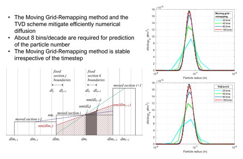
In this study, a sectional moving grid-remapping method for the numerical solution of condensational growth is evaluated. The main novelty of the method is linked with the remapping step, which is based on splitting the particles over all underlying fixed bins, assuming a linear shape for the bin distribution. Extensive comparison with a high resolution TVD (Qamar et al. 2006) and a first order discretization scheme is presented. The method is tested against analytical solutions for pure condensation/evaporation. Further testing is carried out for condensation of sulfuric acid involving a multi-modal distribution. The method is then evaluated for a case of an ideal one-dimensional aerosol reactor, characterized by intense competition of nucleation and growth. The method converges stably and quickly, as the number of bins increases and mitigates numerical diffusion as efficiently as, or even slightly better, than the TVD scheme. The computational cost is comparable to that of the TVD scheme when a Runge-Kutta ODE solver is employed. The number of formed particles is predicted with less than 8 bins/decades. To reproduce all the details of the particle size distribution a higher resolution is needed, mainly due to insufficient density of nodes near the distribution peak. The moving grid-remapping method is independent from convergence conditions. This allows for using a simple explicit time discretization, that reduces the computational cost more than ten times, in the aerosol reactor case. The first order discretization scheme showed extensive numerical diffusion and required more than ten times finer particle size resolution.

Copyright © 2022 American Association for Aerosol Research

Graphical Abstract

EDITOR:

• Yannis Drossinos

Introduction

Aerosol flows and dynamics are of interest in many contemporary scientific, technological, and industrial applications (e.g., Singh et al. 2014; Garcia, Herranz, and Kissane 2016; Mahrukh et al. 2016; Lee, Ha, and Hwang 2017; Herranz et al. 2018; Lee, Cho, and Lim 2019; Zhao, Chen, and Tan 2009; Drossinos and Stilianakis 2020; Netz 2020). Simulation of aerosol dynamics may range from lumped zero-dimensional or one-dimensional approaches to multi-dimensional flow calculations. The latter have significantly benefited from the increased computational power available and are progressively being employed as they can offer a more comprehensive understanding of the spatial and temporal evolution of the various aerosol processes. Several works on multidimensional simulation exist in the literature (e.g., Wilck and Stratmann 1997; Brown et al. 2006; Mitrakos, Hinis, and Housiadas 2007; di Veroli and Rigopoulos 2011; Abarham et al. 2013; Pilou et al. 2013; Sewerin and Rigopoulos 2017a). Nevertheless, multi-dimensional flows modeling may be challenging when stiff aerosol mechanisms are involved (Pyykönen and Jokiniemi 2000; Frederix et al. 2017). Flows in aerosol reactors characterized by strongly competing gas-to-particle aerosol processes i.e., nucleation and condensation, represent such a case. Although individual methods for the numerical treatment of the related terms in the transport equations have been developed over decades (Gelbard, Tambour, and Seinfeld 1980; Pratsinis 1988; Kumar and Ramkrishna 1996a, 1996b, 1997; Whitby and McMurry 1997), modeling capabilities should be further enhanced (Frederix et al. 2017; Woo et al. 2021) and a number of relevant works have been recently published (e.g., Sewerin and Rigopoulos 2017b; Liu and Rigopoulos 2019; Bouaniche, Vervisch, and Domingo 2019; Bouaniche et al. 2020).

In an Eulerian framework, aerosol dynamics are typically treated by two general categories of methods: moment methods and sectional or nodal methods. Moment methods are based on tracking the moments of the particle size distribution, e.g., total particle number or volume, mean particle diameter and standard deviation (Pratsinis 1988). Due to the small number of additional equations, and thus, small computational cost, they are attractive and have been extensively used in multidimensional aerosol flows calculations (Stratmann and Whitby 1989; Wilck and Stratmann 1997; Rosner and Pyykonen 2002; Schwade and Roth 2003; Marchisio, Vigil, and Fox 2003; Brown et al. 2006; Singh et al. 2014; Shiea et al. 2020). Moment methods require approximations for the closure of the moment equations. In its earliest variants the closure was often achieved based on a priori assumption for the shape of the size distribution, such as log-normal (Pratsinis 1988; Whitby and McMurry 1997). Later, in Quadrature Method of Moments (QMOM) method (McGraw 1997; McGraw and Wright 2003; Marchisio, Vigil, and Fox 2003; Marchisio and Fox 2005; Alopaeus, Laakkonen, and Aittamaa 2006) the closure problem is handled numerically, without an a-priori assumption of the distribution function shape. In QMOM, however, the evolved size distribution cannot be straightforward retrieved by the evolution of its moments.

Sectional methods (Gelbard, Tambour, and Seinfeld 1980) are based on dividing the particle size range in finite sections (or bins) and solving the particle transport equation for each bin separately. They are, therefore, capable of directly calculating the evolution of arbitrary distribution shapes. Both the accuracy and the computational cost increase with the number of bins. Methods of this family have also been incorporated and used in the frame of multidimensional flows (Pyykönen and Jokiniemi 2000; Mitrakos, Hinis, and Housiadas 2007; Frederix et al. 2017). Their main drawback is the well-known problem of numerical diffusion, which is a direct result of the numerical discretization of the condensation term in the aerosol transport equation. Numerical diffusion may result in the artificial broadening of the size distribution and thus produce errors in the calculation of the total particle mass evolution. This problem may intensify when very steep modes of particles, formed by nucleation, are appearing during the numerical solution. The numerical diffusion errors, in turn, may have a significant effect on nucleation simulation; the nucleation rate is a very sensitive function of the saturation ratio, which depends on the available vapor concentration in the gas phase and, hence, on the rate with which vapor is depleted by condensation on particles. Increasing the number of the size bins will reduce numerical diffusion and allow for a more accurate simulation of the gas-to-particle processes. This may be feasible in zero- or one-dimensional flows, however, it might be impractical in multi-dimensional flows due to the high additional cost from the large number of bins required (Pyykönen and Jokiniemi 2000; Mitrakos, Hinis, and Housiadas 2007; Garcia, Herranz, and Kissane 2016; Herranz et al. 2018). As it has been indicated by Liu and Rigopoulos (2019), the computational time required for the solution of the additional scalar transport equations in multi-dimensional flows may be significant or even quite larger that the time required for the solution of the flow field. The computational time for the solution of coagulation may also become significant as it is proportional to the square of the number of size bins (Liu and Rigopoulos 2019). Moreover, in multi-dimensional flows, the calculations may involve a very large number of numerical iterations (either in steady state or transient cases) to reach a solution. The errors due to the numerical diffusion propagate and accumulate during these iterations. To compensate these accumulated errors an even larger number of size bins is required further increasing the cost of multi-dimensional calculations. It is therefore important that a sectional or discretization method can mitigate efficiently numerical diffusion with a low number of bins.

It is well known that first order discretization of the condensation term, such as an upwind scheme, ensures stability, however it also suffers from extensive numerical diffusion. Higher order methods can reduce significantly numerical diffusion, but they may introduce discontinuities in the solution (Kumar and Ramkrishna 1997; Hounslow, Ryall, and Marshall 1988; Park and Rogak 2004), which may lead to overshoots or instabilities and divergence. Nevertheless, high resolution schemes, originally developed for gas flow resolution, such as the Total Variation Diminishing (TVD) scheme, have been adjusted and used successfully for the solution of population balances (Gunawan, Fusman, and Braatz 2004; Qamar et al. 2006). TVD schemes are much more accurate than the first order schemes and, by using appropriate flux limiters, they can retain stability. The so called $k=1/3$ TVD scheme, proposed by Qamar et al. (2006), has recently been employed for the solution of the Population Balance Equation (PBE) in the context of CFD for a two-dimensional simulation of soot formation in a laminar flame (Liu and Rigopoulos 2019). Another family of methods include the moving grid methods (Kim and Seinfeld 1990) or the methods of characteristics (Kumar and Ramkrishna 1996b, 1997). In these methods, particle size bins are allowed to move along the particle size dimension, following the growth rate. Consequently, the evolution of the size distribution can be captured very accurately during growth, including when very sharp shapes are involved. If particle formation via nucleation occurs, care has to be taken during moving of the grids to add new bins for accommodating the newly formed particles. This process may increase significantly the computational cost (e.g., Roussos, Alexopoulos, and Kiparissides 2006). A more significant problem for these methods is that they cannot be directly used in an Eulerian transport framework. This is because the size of the bins may vary, creating inconsistencies throughout the spatial and temporal computational domain (Zhang et al. 1999; Sewerin and Rigopoulos 2017b).

Moving grid methods are usually combined with a technique for remapping the moved distribution back to a fixed particle size grid, where all other processes and especially transport can be straightforward solved. These moving grid-remapping methods, which originally developed for atmospheric models (Lurmann et al. 1997) have been also employed in internal aerosol flows (Mitsakou, Helmis, and Housiadas 2004) including in the frame of CFD calculations (Mitrakos, Hinis, and Housiadas 2007). One of the most efficient methods of this type in combating numerical diffusion is the so-called moving center method (Jacobson 1997). In this method, all particles of a moved bin are added to the fixed one, where the average size of the moved bin lies. This way the particle number is conserved. Total particle volume is also conserved by calculating a new characteristic size of each bin by averaging the volume of the particles of all bins added into it. The method eliminates numerical diffusion, but it may create empty bins and artificially discontinuous particle size distributions. Even if this issue is resolved (Mohs and Bowman 2011), still, the implementation of the moving center method is not straightforward in CFD calculations due to the spatial inconsistency of the particle size (Zhang et al. 1999). In our earlier work (Mitrakos, Hinis, and Housiadas 2007), a different approach was proposed for remapping the distribution, based on spline interpolation on the cumulative distribution (Yamamoto 2004, 2012) instead of the size distribution itself. The method performed well for very sharp distributions and strong coupling of nucleation and condensational growth, however, neither the particle number nor the volume were inherently conserved.

More advanced methods have been also developed based on adaptive grid approaches. These methods are based on dynamically refining the particle size grid in regions where intense changes of the distribution take place and coarsening it elsewhere. Qamar et al. (2007) employed an adaptive method based on the moving mesh technique of Tang and Tang (2003) and Tang (2005), whereby the total number of the mesh nodes is conserved. In this method, solution of the PBE is carried out in two steps. First the mesh is moved according to a smooth monitor function and then the PBE is numerically solved to obtain the solution on the moved particle size mesh. The method performed very well, in particular when the high resolution TVD scheme was used for the solution of growth. However, implementation of the method in an Eulerian framework is not straightforward, as the moved particle size mesh may vary inducing inconsistencies throughout the temporal and spatial domain, as already mentioned above for the case of the moving grid methods. Sewerin and Rigopoulos (2017b) developed an advanced adaptive grid method, where the whole PBE is transformed based on a particle size coordinate transformation, which is space and time dependent. In this case, consistency of the particle distribution in space and time is ensured by varying the parameterization of the distribution, through a common transformed coordinate, which is consistent across the spatial domain (Sewerin and Rigopoulos 2017b). The method was tested with different numerical schemes for the solution of the transformed PBE, including also the $k=1/3$ TVD scheme, which provided excellent performance, almost eliminating numerical diffusion. Finally, Monte Carlo methods have also been proposed for the solution of the PBE. Although, these methods were originally very time demanding, latest development, indicatively by Bouaniche, Vervisch, and Domingo (2019) and Bouaniche et al. (2020) demonstrated efficient mitigation of numerical diffusion and showed promising evidence that they can be further implemented for the solution of multi-dimensional problems.

In this work, we present a simple, novel method for the numerical solution of condensational growth, which belongs to the family of the moving grid-remapping methods. The method presents some improved attributes. The remapping step is carried out in a physically consistent way, by sharing the particles of a moved bin between all fixed bins which the moved one overlaps. In addition, sharing of particles is carried out assuming that the size distribution within the moved bin follows a linear shape, with its slope approximated using the values of the moved distribution at the adjacent moved bins. By its construction, the method conserves the number of particles. Extensive validation and evaluation of the method is presented against different cases representing a wide range of condensation conditions. Initially the method is validated against well-known analytical solutions for condensation in a case involving sharp (close to monodisperse) particle size distribution. Further testing is performed for a theoretical case of sulfuric acid condensation, where evolution of a multimodal, instead of unimodal, distribution is involved. To evaluate the performance of the method in cases characterized by strong nucleation-condensation coupling, one-dimensional simulation of an aerosol reactor flow is examined for a theoretical case of CsOH nucleation and growth available in the literature. Extensive comparison is also carried out by performing calculations with the high resolution $k=1/3$ TVD scheme of Qamar et al. (2006). The effect of the method that is used for the time integration of the involved equations is also evaluated. In particular, two methods were used, a robust Runge-Kutta ODE and a simple direct explicit time discretization. Calculations with a first order discretization scheme were also employed, serving as a reference to provide a tangible picture of the numerical diffusion issue.

Model description

Before the description of the numerical method, we provide representative laws for homogeneous nucleation and condensational growth.

Nucleation and condensational growth expressions

Aerosol transport and dynamics are described by a PBE (e.g., Ramkrishna 2000), also known as the General Dynamic Equation (Friedlander 2000). Focusing solely on condensational growth and nucleation, the equation is written: (1) $$\frac{\partial n}{\partial t}={\left.\frac{\partial n}{\partial t}\right|}_{\mathit{growth}}+\mathrm{}{\left.\frac{\partial n}{\partial t}\right|}_{\mathit{nucl}}=-\frac{\partial Gn}{\partial d}+J\delta (d-d_{\mathit{crit}})$$(1)

In this equation, $n$ is the particle number size distribution function or number density (particles μm⁻¹ m³), $d$ the particle diameter (μm), $G$ the particle growth rate (μm/s), $J$ the nucleation rate (particles m⁻³ s⁻¹), $d_{c\mathrm{r}it}$ the critical diameter of particles generated by nucleation and $\delta$ the Dirac function. Growth of existing particles due to condensation of vapor onto their surface is described separately for the molecular (small particles with Knudsen number Kn = λ/r ≫1) and the continuous regime (large particles, Kn = λ/r ≪ 1). Typically, a single expression, based on appropriate interpolation, is employed for both extremes and the transition regime in-between. The equation depicts a particle growth rate inversely proportional to the diameter. An often-used expression, accounting for both heat and mass transfer between the particle and the surrounding gas phase, is based on a modified Mason equation (Mason 1971) with a Fuchs-Sutugin correction (Jokiniemi et al. 1994; Mitrakos, Hinis, and Housiadas 2007): (2) $$G\left(d\right)=\mathrm{}\frac{dd}{dt}=\frac{4}{{\rho }_{p}d}\left(\frac{S-1}{\frac{f_{\mathit{mass}}}{F_{FS}^{\mathit{mass}}}+\frac{f_{\mathit{heat}}}{F_{FS}^{\mathit{heat}}}}\right)$$(2)

In this equation, $S$ is the surrounding vapor saturation ratio for a flat surface and ${\rho }_p$ the density of the particles. To correct for the increased supersaturation due to the curved particle surface, the Kelvin effect may be included in the growth law (see for example Hinds 2012). $f_{\mathit{mass}}$ and $f_{\mathit{heat}}$ account for mass and heat transfer between the particle and the surrounding air-vapor mixture, corrected by the corresponding Fuchs-Sutugin correction factor, $F_{FS},$ which is a function of vapor and carrier gas Knudsen numbers, respectively.

Various expressions have been proposed for the prediction of the homogeneous nucleation rate. One of the most commonly used is derived from the classical nucleation theory (Frenkel 1955). In this theory, the rate ($J_{\mathit{class}}$) at which particles of critical diameter, $d_{\mathit{crit}},$ are formed is given by: (3) $$J_{\mathit{class}}=\frac{C^2}{{\rho }_p{m}_m}\sqrt{\frac{2\sigma }{\pi m_m}}\exp \left(-\frac{\pi \sigma d_{\mathit{crit}}^2}{3k_{B}T}\right),\mathrm{}{\mathrm{}d}_{\mathit{crit}}=\frac{4\sigma {\upsilon }_m}{k_{B}T\ln \left(S\right)}$$(3) where, $C$ is the condensable vapor concentration in the gas phase, $T$ the temperature of the gas, $\sigma$ the surface tension, ${\upsilon }_m\mathrm{}$ and $m_m$ the condensable species molecular volume and mass, respectively, and $k_B$ the Boltzmann constant.

Numerical treatment

Numerical treatment of the nucleation term in the context of a sectional representation with fixed particle size grid is straightforward. It can be easily resolved by adding the particles formed within a timestep to the bin within which the critical diameter ($d_{\mathit{crit}}$) lies. On the contrary, as already mentioned, several approaches have been proposed for growth solution, each with its own advantages and shortcomings. In this work, besides the moving grid-remapping method, we also perform calculations with two discretization schemes; a first order discretization scheme and a high resolution TVD scheme that have been used in the literature for the solution of the PBE. We first provide a short description of the discretization schemes and then we describe in detail the present moving grid-remapping method.

Discretization schemes

First order discretization has been used for PBE solution in multidimensional flows (e.g., Pyykönen and Jokiniemi 2000), or it has been employed as the solver for particle growth in multipurpose CFD codes, e.g., in ANSYS Fluent (Ansys, Inc. 2019). Expressed in terms of volume concentration ($V_i),$ with particle volume as the independent variable, such a discretized equation for a bin $i$ can be written as follows (Hounslow, Ryall, and Marshall 1988; Pyykönen and Jokiniemi 2000; Ansys, Inc. 2019): (4) $${\left.\frac{d{V}_i}{dt}\right|}_{\mathit{growth}}=G_{v,i-1}\frac{N_{i-1\mathrm{}}{v}_{i-1}}{v_i-v_{i-1}}-G_{v,i}\frac{N_i{v}_i}{v_{i+1}-v_i}$$(4)

In the above equation, $G_{v,i}$ is the volumetric growth rate (μm³/s) of particles with volume $v_i$ and $N_i\mathrm{}(=V_i/v_i)$ the number concentration (particles/m³) of the bin$\mathrm{}i.$ The above scheme, despite its simplicity and stability, presents a very important, well-known drawback. It produces extensive numerical diffusion during solution of condensational growth.

Higher order, high resolution TVD schemes have been also proposed (Gunawan, Fusman, and Braatz 2004; Qamar et al. 2006) and have been recently employed successfully in CFD for the simulation of soot formation in laminar flame (Liu and Rigopoulos 2019). The authors, in the latter work, extended the use of the finite volume high resolution TVD scheme, initially developed by Qamar et al. (2006) for uniform particle size grids, to non-uniform grids. In the present work, we also selected the above TVD scheme as a representative high resolution scheme. The purpose was to evaluate its performance and compare it with the present moving grid-remapping method. The TVD scheme, with the diameter as the independent particle size variable, can be written as follows (Qamar et al. 2006; Liu and Rigopoulos 2019): (5) $$\frac{\partial n_i}{\partial t}+\frac{1}{\Delta d_i}\left({\left(Gn\right)}_{d_i^{+}}-{\left(Gn\right)}_{d_i^{-}}\right)=\frac{J\left(t\right)\delta (d-d_{\mathit{crit}})}{\Delta d_i}$$(5)

The two finite volume cell fluxes $(Gn)$ are approximated by using the formula with an interpolation factor $k=1/3,$ which results to a weighted combination between the 2^nd order central scheme and the 1^st order upwind scheme. The flux at the right cell face ($d_i^{+}$) is given by (Qamar et al. 2006): (6) $$\begin{array}{c}{\left(Gn\right)}_{d_i^{+}}=G_{d_i^{+}}\left(n_i+\frac{1}{2}\Phi \left(r_i^{+}\right)\left(n_i-n_{i-1}\right)\right)\\ r_i^{+}=\frac{n_{i+1}-n_i+\epsilon }{n_i-\mathrm{}{n}_{i-1}+\epsilon }\end{array}$$(6)

The left cell flux is approximated similarly. In the above equation, $\epsilon$ is a small constant introduced to avoid division by zero. The flux limiter, $\Phi ,$ in the above scheme is a function of the values of the distribution itself, thus rendering the system of Equations (5)(5) $$\frac{\partial n_i}{\partial t}+\frac{1}{\Delta d_i}\left({\left(Gn\right)}_{d_i^{+}}-{\left(Gn\right)}_{d_i^{-}}\right)=\frac{J\left(t\right)\delta (d-d_{\mathit{crit}})}{\Delta d_i}$$(5) non-linear. The equations can be solved by explicit time discretization (Gunawan, Fusman, and Braatz 2004) or by employing an ODE solver, e.g., a Runge-Kutta method as in Qamar et al. (2006).

Moving grid-remapping method

The method introduced in this work is based on a moving grid-remapping approach. Examples of these methods can be found in the works of Lurmann et al. (1997), Jacobson (1997), Mitrakos, Hinis, and Housiadas (2007), and Mitsakou, Helmis, and Housiadas (2004). In this family of methods, the solution of growth in each timestep is carried out separately from the other processes, by utilizing an operator-splitting approach. The solution of growth in each timestep consists of two successive steps: First, the growth equation is integrated for all particle size bins boundaries, so that the new position of each bin in the particle size coordinate at the end of the timestep is evaluated. This step, which comprises the moving grid step, produces the so-called “moved” size distribution, i.e., the size distribution expressed on the moved particle size grid, and is characteristic of the family of the moving grid methods mentioned above. In the second step, the moved distribution is remapped back to the fixed particle size grid, where the other aerosol process, and especially transport, can be solved. The procedure for the remapping of the distribution comprises the novelty of the approach introduced in this article. In the remaining of this section, we describe the above two steps in more detail.

The moved number distribution of bin $i,$ ${nm}_i,$ at the end of the timestep ($\Delta t)$ is evaluated in the moving grid step, as follows. The moved boundaries of bin $i\mathrm{}$ at the end of the timestep, namely ${\mathit{dlm}}_i$ and ${\mathit{dlm}}_{i+1},$ are calculated by numerically integrating the growth law equation (e.g., Equation (2)(2) $$G\left(d\right)=\mathrm{}\frac{dd}{dt}=\frac{4}{{\rho }_{p}d}\left(\frac{S-1}{\frac{f_{\mathit{mass}}}{F_{FS}^{\mathit{mass}}}+\frac{f_{\mathit{heat}}}{F_{FS}^{\mathit{heat}}}}\right)$$(2) ) for all bins boundaries: (7) $${\mathit{dlm}}_i={\int }_0^{\Delta t}G\left(d\right)dt,\mathrm{}{d}_{t=0}={dl}_i,\mathrm{}i=1,\dots ,\mathit{nbin}+1$$(7) where ${dl}_i$ is the left boundary of the fixed bin $i.$ The same applies for the right boundary, ${dl}_{i+1},$ as well. As in the fixed grid, the characteristic size of each moved bin (${dm}_i$) is specified at the middle of the bin (arithmetic mean of the bin boundaries). During growth, the number of particles is conserved. Therefore, the number density on the moved grid can be directly calculated as: (8) $${nm}_i=n_i^0\frac{\left({dl}_{i+1}-{dl}_i\right)}{\left({\mathit{dlm}}_{i+1}-{\mathit{dlm}}_i\right)}$$(8)

In the above equation, $n_i^0$ and ${nm}_i$ are the particle size number density values of bin $i$ before and after growth, respectively ($m$ is used to denote the moved number density). Equation (8)(8) $${nm}_i=n_i^0\frac{\left({dl}_{i+1}-{dl}_i\right)}{\left({\mathit{dlm}}_{i+1}-{\mathit{dlm}}_i\right)}$$(8) expresses the conservation of the number of particles for each size bin during growth. It should be noted that if evaporation takes place, particles may be evaporated out of the lower limit of the size range, so they are removed from the distribution. Apparently, the number of particles is not conserved in this case.

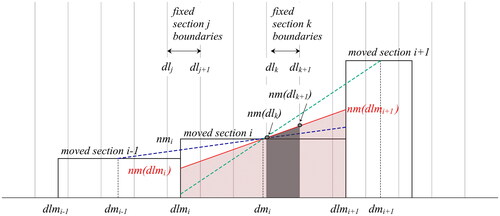
After the moving grid step, it is necessary to remap the moved size distribution back to the fixed particle size grid. In previous approaches with this type of methods, remapping was performed based on polynomial interpolation, e.g., spline (Lurmann et al. 1997; Mitsakou, Helmis, and Housiadas 2004; Mitrakos, Hinis, and Housiadas 2007) or by splitting the particles of a moved bin to the fixed bins adjacent to the characteristic moved diameter (e.g., Jacobson 1997). The most important drawback of interpolation methods is that they do not ensure number conservation, which is a physically consistent condition during growth. On the other hand, splitting the particles to two adjacent bins, although it can be made by imposing conservation of number and/or volume of particles, may also create significant numerical diffusion. In this article, we introduce a new approach for the remapping step. The particles contained in a moved bin are distributed among all fixed grid bins that the moved one crosses, thus ensuring particle number conservation. In addition, to reduce numerical diffusion during the remapping step, we assume that each moved bin holds a linear, trapezoid-like shape. To facilitate understanding of the method, we present the remapping step based first on a histogram-like shape and then we introduce the trapezoid-like approach.

A fictitious picture of some moved bins and their number distribution ($nm),$ after the moving grid step, is provided in Figure 1. The fixed particle size grid is also shown in the figure. In general, different possible positions of the moved bins with reference to the fixed grid may be anticipated. It is possible, for example, that a moved bin lies entirely within the limits of a single fixed one. This is a favorable case, in which all particles of the moved bin can be directly added to the fixed section. Adding all particles to the fixed bin, in which they are contained, is a physically consistent treatment that conserves the number of particles. It also eliminates numerical diffusion, which otherwise would appear if particles were split in adjacent bins. In the general case, however, the picture may be more complicated, with the moved size bins crossing over more than one fixed bins, as shown in Figure 1. In this case, an approach to split the moved particles to all underlying fixed bins is required. The simplest approach could rely on a histogram-like rectangular shape of the distribution (bold black lines) and allocate to each fixed bin the segment of the moved one that lies over it. For example, the particle number concentration added to the fixed bin $k,$ from the segment of the moved bin $i$ that falls within the “internal” fixed bin $k$ would be calculated as: (9) $${\Delta N}_{i\to k}={nm}_i\left({dl}_{k+1}-{dl}_k\right)$$(9) or for a bin at the edge (e.g., bin $j$) (10) $${\Delta N}_{i\to j}={nm}_i\left({dl}_{j+1}-{\mathit{dlm}}_i\right)$$(10)

Figure 1. A schematic description of the moved particle size distribution remapping to the fixed grid. The fixed particle size grid is shown with gray lines, while a fictitious snapshot of three moved bins is depicted with the bold black lines. The blue and green dotted lines denote the approximated backward and forward slopes of the distribution and the red line, in between, the average slope, which we use to approximate the shape (red shaded trapezoid) of the distribution within the moved section. The area formed by the gray shaded trapezoid within each fixed bin represents the particles added to it in a time-step.

Although, this is a simple and straightforward option, yet it would also lead to artificially overspreading of the particle number distribution and thus introduce significant numerical diffusion.

An alternative, simple approach is to assume that the distribution varies linearly within each moved section. The slope of the line can be calculated by the values of the moved distribution at the adjacent bins, thus, taking advantage of the actual shape of the distribution in the vicinity of the moved bin. The slope of the distribution (bold red line) inside a moved bin $i$ is calculated as the average of the backward (blue line) and forward (green line) slopes, using the following equation: (11) $${sl}_i=\left(\frac{{nm}_i-{nm}_{i-1}}{{dm}_i-{dm}_{i-1}}+\frac{{nm}_{i+1}-{nm}_i}{{dm}_{i+1}-{dm}_i}\right)/2$$(11)

The shape of the particle size distribution within the moved bin is thus specified by the line, which passes from the middle of the moved bin $i,$ i.e., from the point (${dm}_i,$ ${nm}_i)$ and has a slope given by Equation (11)(11) $${sl}_i=\left(\frac{{nm}_i-{nm}_{i-1}}{{dm}_i-{dm}_{i-1}}+\frac{{nm}_{i+1}-{nm}_i}{{dm}_{i+1}-{dm}_i}\right)/2$$(11) . The particle number of the moved bin is equal to the area of the trapezoid (shadowed in red) formed by that line, the particle size axis, and the boundaries of the bin. The particle number is conserved, provided that the line passes through the middle of the bin. This condition can be directly met by defining the characteristic particle size of each bin (diameter ${dm}_i$ for the moved bin $i$ in Figure 1) at the middle of the bin, as is often made in constructing the particle size grid.

Implementation of the method includes the following. In each timestep, the moved boundaries of all bins are first calculated by numerically integrating Equation (7)(7) $${\mathit{dlm}}_i={\int }_0^{\Delta t}G\left(d\right)dt,\mathrm{}{d}_{t=0}={dl}_i,\mathrm{}i=1,\dots ,\mathit{nbin}+1$$(7) . We then determine the fixed bins, across which each moved one overlaps. If a moved bin is entirely contained in a single fixed one, then all particles of the moved bin are added into this single fixed bin. Otherwise, if a moved bin crosses more than one fixed bins, then its particles are distributed to the fixed bins according to the trapezoidal shape described in the previous paragraph. This is equivalent to adding into the fixed bins the area of the segment of the trapezoid (the area, shadowed in gray in Figure 1). Therefore, the increment of the particle number concentration of the “internal” fixed bin $k,$ due to the contribution of the moved bin $i,$ is given by: (12) $$\Delta N_{i\to k}=\frac{nm\left({dl}_{k+1}\right)+nm\left({dl}_k\right)}{2}\left({dl}_{k+1}-{dl}_k\right)$$(12) where, the values of the moved distribution at the boundaries of the fixed bin are calculated by linear interpolation with the slope defined in Equation (11)(11) $${sl}_i=\left(\frac{{nm}_i-{nm}_{i-1}}{{dm}_i-{dm}_{i-1}}+\frac{{nm}_{i+1}-{nm}_i}{{dm}_{i+1}-{dm}_i}\right)/2$$(11) above: (13) $$nm\left({dl}_k\right)={nm}_i+{sl}_i\left({dl}_k-{dm}_i\right)$$(13)

The increment of particles to the “edge” fixed bins (e.g., $j$ in Figure 1) are calculated similarly, with the difference that the trapezoid is defined in this case by only one of the sides of the fixed bin and one side of the moved bin: (14) $$\Delta N_{i\to j}=\frac{nm\left({dl}_{j+1}\right)+nm\left({\mathit{dlm}}_i\right)}{2}\left({dl}_{j+1}-{\mathit{dlm}}_i\right)$$(14)

To avoid unrealistic negative values of the calculated distribution, limiting values are imposed to the calculated slopes of the assumed inclined line. The corresponding conditions are: (15) $$\begin{array}{c}{sl}_i=\mathit{min}\left({sl}_i,{sl}_{i,\mathit{limit}}^{\mathit{west}}\right),\mathrm{}if\mathrm{}{sl}_i>0\\ {sl}_i=-\mathit{min}\left(\left|{sl}_i\right|,\left|{sl}_{i,\mathit{limit}}^{\mathit{east}}\right|\right),\mathrm{}if\mathrm{}{sl}_i<0\end{array}$$(15)

These conditions ensure that the inclined line does not transcend the horizontal axis and thus does not produce negative values in the west or the east side, depending on the sign of the slope. The limiting slopes are given by: (16) $$\begin{array}{c}\mathrm{}{sl}_{i,\mathit{limit}}^{\mathit{west}}=\mathrm{}\frac{{nm}_i}{{dm}_i-{\mathit{dlm}}_i}\\ {sl}_{i,\mathit{limit}}^{\mathit{east}}=\mathrm{}\frac{-{nm}_i}{{\mathit{dlm}}_{i+1}-{dm}_i}\end{array}$$(16)

The process described above is repeated for all non-zero moved bins, so that the whole moved distribution is remapped back to the fixed particle size grid in each timestep.

Validation tests for condensation

The method was first validated by comparing its predictions with available, well-known analytical solutions of the general dynamic equation for condensation and evaporation (Seinfeld and Pandis 2006). The particle size distribution function has initially the form of a log-normal distribution, given by: (17) $$n_0=\frac{N_0}{\sqrt{2\pi }\mathrm{l}\mathrm{n}\left({\sigma }_{{\rm I}}\right)}\mathrm{e}\mathrm{xp}\left(-\frac{{ln}^2\left(d_p/d_{pI}\right)}{2{ln}^2\left({\sigma }_{{\rm I}}\right)}\right)\frac{1}{d_p}$$(17)

In the above equation, $N_0$ is the total number concentration, $d_{pI}$ the mean particle diameter and ${\sigma }_{{\rm I}}$ the geometric standard deviation. The particles grow (or evaporate) according to an inverse diameter growth law, given by the following equation: (18) $$\frac{d{d}_p}{dt}=\frac{A}{d_p}$$(18) with $A$ denoting a condensation constant (${\mathrm{cm}}^{-2}{\mathrm{s}}^{-1}$).

The analytical solution for this problem is given by the following equation (Seinfeld and Pandis 2006): (19) $$n(d_p,\mathrm{t})=\frac{d_p}{\left({d_p}^2-2At\right)}\frac{N_o}{\sqrt{2\pi }\mathrm{}\ln \left({\sigma }_{{\rm I}}\right)}\mathrm{e}\mathrm{xp}\left(-\frac{{\ln }^2\left[{\left({d_p}^2-2At\right)}^{1/2}/d_{pI}\right]}{2{\ln }^2\left({\sigma }_{{\rm I}}\right)}\right)$$(19) Two cases were examined. The first refers to pure condensation, whereas the second to pure evaporation. Regarding condensation, a case with initial median diameter $d_{pI}=0.1\mathrm{\mu }\mathrm{m},$ initial standard deviation ${\sigma }_{{\rm I}}=1.15$ and condensation constant $A={10}^{-10}\mathrm{}{\mathrm{cm}}^{-2}{\mathrm{s}}^{-1}\mathrm{}$ is considered. Simulation is performed for a total time $T_f=1\mathrm{s},$ at the end of which, a very narrow distribution is obtained because the above growth law tends to a monodisperse distribution with time. The particle size grid used in the numerical calculations extends from a minimum particle diameter equal to $0.01\mathrm{}\mathrm{\mu }\mathrm{m}$ to a maximum of $1.0\mathrm{}\mathrm{\mu }\mathrm{m}.$ For both methods employed for this case, i.e., the moving grid-remapping method and the TVD scheme, a fourth-order Runge-Kutta ODE solver, available in Matlab, was used for the solution of the differential equations (Equation (7)(7) $${\mathit{dlm}}_i={\int }_0^{\Delta t}G\left(d\right)dt,\mathrm{}{d}_{t=0}={dl}_i,\mathrm{}i=1,\dots ,\mathit{nbin}+1$$(7) for the moving grid-remapping method and Equation (5)(5) $$\frac{\partial n_i}{\partial t}+\frac{1}{\Delta d_i}\left({\left(Gn\right)}_{d_i^{+}}-{\left(Gn\right)}_{d_i^{-}}\right)=\frac{J\left(t\right)\delta (d-d_{\mathit{crit}})}{\Delta d_i}$$(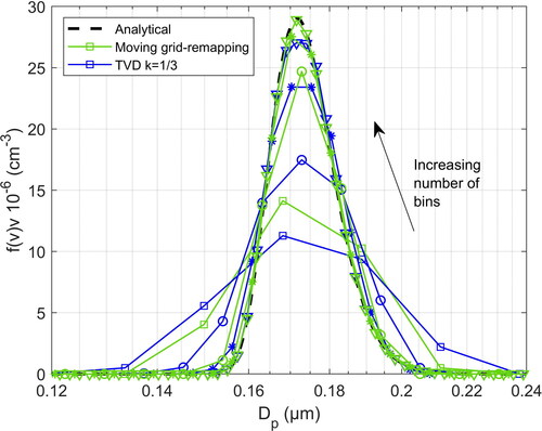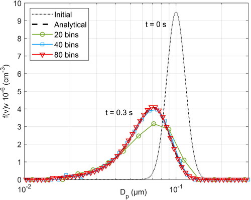5) for the TVD scheme). In Figure 2, the calculated particle number distribution is shown as calculated using different particle size resolutions. For comparison, the analytical solution is also shown. It can be observed that the numerical results converge steadily to the analytical solution, as the number of the particle size bins increases. During the time marching iterations, the total number concentration of the particles was exactly conserved in the numerical solution, as expected for pure condensation, irrespectively of the number of bins. As mentioned previously, as the number of numerical solution iterations increases, the numerical errors, and especially those related to numerical diffusion, may accumulate as the solution evolves. If these errors are large, an even larger number of bins will be needed to retain the same degree of accuracy as the number of iterations increases, i.e., for lower time steps. For this reason, we also tested the accuracy and the behavior of the method by using different time steps. However, no visible differences or any change in the stability of the calculations were noticed when a time step one order of magnitude lower was used. Another observation is that some numerical diffusion appears when a small number, namely 20 or 40 bins are used. Numerical diffusion, however, diminishes very quickly and practically vanishes as the number of bins increases to 80 bins (40 bins/decade). In Figure 3, the distribution, as calculated with the moving grid-remapping method is compared with the results using the TVD scheme. Both methods present a favorable behavior and combat efficiently numerical diffusion as the number of bins increases. We can observe only some small differences, with the TVD scheme depicting a slightly slower convergence compared to the moving grid-remapping method, as the number of bins increases.

Figure 2. Numerical results for the particle number distribution at $T_f=1\mathrm{}s$ for pure condensation, as calculated with the present method for varying number of bins, in comparison with the analytical solution.

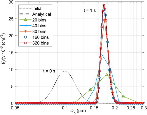
Figure 3. Comparison of the convergence between the present method and the high resolution finite volume TVD scheme of Qamar et al. (2006) for the case of Figure 2, using 40, 80, 160 and 320 particle size bins. Lines with the same marker denote the same number of bins.

The second case focused on the evolution of the particle size distribution under the influence of pure evaporation. The same log-normal initial distribution used for condensation was also assumed. The condensation constant in this case is taken equal to $A=-{10}^{-10}\mathrm{}{\mathrm{cm}}^{-2}{\mathrm{s}}^{-1},\mathrm{}$ whereas simulations were performed for a total simulation time $T_f=0.3\mathrm{}\mathrm{s}.$ The numerical results for different number of bins are presented in Figure 4, along with the analytical solution. In this case, a significantly lower number of bins is required for the numerical results to converge and achieve an excellent agreement with the analytical solution. This is directly related with the reverse behavior of the distribution when evaporation occurs. More specifically, as particle shrinks, the distribution moves toward smaller diameters. Since smaller particles evaporates - i.e., move toward lower particle sizes - faster than the larger ones, the distribution spreads with time. This spreading, as opposed to the narrowing behavior in condensation, allows the numerical solution to capture more easily the shape of the distribution with only a small number of bins. It must be noted that in this case the total particle number is not conserved, because the particles that outreach the lower limit of the size range are removed from the distribution. In agreement with the case of pure condensation, no significant differences were observed when more time steps, as previously, were used, indicating that the accumulated errors are again small.

Figure 4. Numerical results for the particle number distribution at $T_f=0.3\hspace{0.17em}\mathrm{s}$ for pure evaporation, as calculated, with the present method for varying number of bins, in comparison with the analytical solution.

The pure condensation case analyzed in the previous paragraphs, although relatively challenging due to the very narrow distribution of particles, is associated with a unimodal distribution. In real applications, however, bi- or multi-modal distributions may appear (see for example Kissane et al. 2009) when gas-to-particle conversion occurs through nucleation and condensation. As an example of a multi-modal distribution, we examined the case presented in Seigneur et al. (1986) and Zhang et al. (1999). This case concerns condensation of sulfuric acid on an initially three-mode (Aitkin, accumulation and coarse particle mode) particle distribution. Among the numerical cases examined in Seigneur et al. (1986) and Zhang et al. (1999), we selected one corresponding to hazy conditions, which is the most challenging to reproduce numerically due to the sharp growth of the nucleation mode. The growth rate with the Fuchs-Sutugin correction formula, used in the referenced works, is also incorporated here. For the purposes of the current calculations, the growth rate is written in a convenient manner, as follows (Yamamoto 2004): (20) $$\frac{dv}{dt}=\frac{r}{1+\left(\frac{1.333Kn+0.71}{1+Kn}\right)Kn}B$$(20)

In this equation, $r$ is the particle radius and $Kn$ the particle Knudsen number. The condensation parameter $B$ encompasses the influence of the condensable species properties and the prevailing saturation conditions. Its value is specified, so that a total volume of 5.5 μm³ cm⁻³ of sulfuric acid is condensed in 12 h. To obtain the exact solution, we follow the approach used in Zhang et al. (1999), whereby the problem was solved using a moving grid numerical technique. Here, we obtained the exact final distribution by solving the general dynamic equation with the moving grid approach described previously (see Equations (7)(7) $${\mathit{dlm}}_i={\int }_0^{\Delta t}G\left(d\right)dt,\mathrm{}{d}_{t=0}={dl}_i,\mathrm{}i=1,\dots ,\mathit{nbin}+1$$(7) and (8)(8) $${nm}_i=n_i^0\frac{\left({dl}_{i+1}-{dl}_i\right)}{\left({\mathit{dlm}}_{i+1}-{\mathit{dlm}}_i\right)}$$(8) ).

Τhe results using the present method and the TVD scheme are provided in Figures 5 and 6, respectively. In Figure 7, the results with the first order discretization scheme are shown, as a reference that helps to obtain a picture of the effect that the numerical diffusion has on capturing the evolution of the nucleation mode. A particle size range from 0.01 μm to 100 μm was used in the calculations for all methods. The initial volume distribution, calculated following Zhang et al. (1999) by assuming that each mode can be represented by a lognormal function (see Equation (3)(3) $$J_{\mathit{class}}=\frac{C^2}{{\rho }_p{m}_m}\sqrt{\frac{2\sigma }{\pi m_m}}\exp \left(-\frac{\pi \sigma d_{\mathit{crit}}^2}{3k_{B}T}\right),\mathrm{}{\mathrm{}d}_{\mathit{crit}}=\frac{4\sigma {\upsilon }_m}{k_{B}T\ln \left(S\right)}$$(3) therein), is also depicted. As it is observed, growth of the nucleation mode results to the narrow mode located around about 0.09 μm. The numerical solution reproduces very well the rest of the distribution, even with a low number of bins. To capture the sharp growth of nucleation mode, however, 80 or more bins are required. In this case also, it can be noticed that the moving grid-remapping method captures the details of the distribution somewhat better for the same number of bins. This may comprise evidence of a slightly more efficient mitigation of numerical diffusion. We must note, however that to capture the narrow nucleation node, in the context of a fixed sectional representation, it is necessary that an adequate number of fixed bins exist at the mode. Thus, the apparent inability to capture graphically the nucleation mode with less bins, in both methods, is mostly related with the lack of nodes at the nucleation mode sizes and less with numerical diffusion. We should note that an adaptive grid technique, as those developed in Qamar et al. (2007) or Sewerin and Rigopoulos (2017b), could capture more efficiently such sharp and narrow modes of the distribution, by progressively refining the grid size resolution in the vicinity of the mode. The effect of numerical diffusion is clearly shown in Figure 7 where the results with the first order discretization scheme are presented. It is evident that an extremely fine particle size resolution is required to capture the existence of the narrow nucleation mode. Compared to the previous schemes, to achieve a similar accuracy in reproducing the details of the distribution, more than 1000 bins are required i.e., one order of magnitude finer resolution compared to that needed with the moving grid-remapping method or the high resolution TVD scheme.

Figure 5. Particle volume distribution after condensation of sulfuric acid for 12 h, as calculated with the present moving grid-remapping method, for different number of bins.

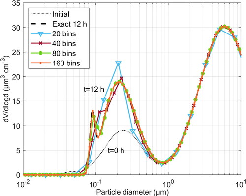
Figure 6. Particle volume distribution after condensation of sulfuric acid for 12 h, as calculated with the high resolution finite volume TVD scheme, for different number of bins.

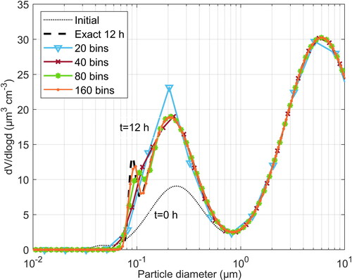
Figure 7. Particle volume distribution after condensation of sulfuric acid for 12 h, as calculated with a first order discretization scheme, for different number of bins.

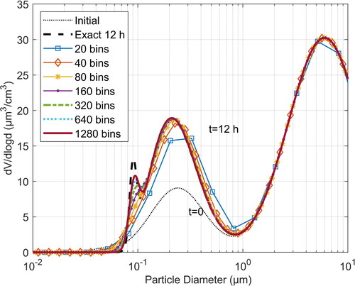
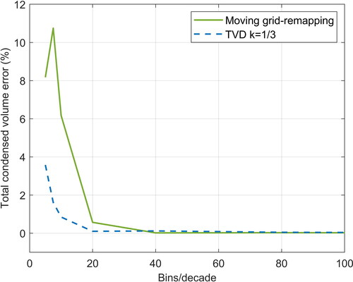
As already mentioned, the moving grid-remapping method conserves the total number of particles but not the volume of the distribution. Figure 8 shows the error in the calculation of the total condensed volume of sulfuric acid for the moving grid-remapping method and the TVD scheme. It is observed that the TVD scheme depicts significantly smaller errors, compared with the present method, for small number of bins. However, the errors of the moving grid-remapping method very quickly decrease, and are very small (<1%) for 20 bins/decade while are eliminated at less than 40 bins/decade.

Figure 8. Error in calculation of the total volume of condensed sulfuric acid, as a function of the particle size resolution using the moving grid-remapping method and the high resolution TVD scheme.

Evaluation for strongly coupled nucleation and growth

In the following, the results of the application of the present method in a case involving homogeneous nucleation-condensation in an aerosol reactor are presented. The case, which has been examined also in the works of Pyykönen et al. (2002) and Brown et al. (2006), deals with the generation of CsOH particles via homogeneous nucleation and condensation in a theoretical, one-dimensional aerosol reactor. An air-CsOH vapor mixture flows in the reactor, where it is cooled. The cooling of the mixture causes high supersaturation of the CsOH vapor in the gas phase and subsequent particle formation by homogeneous nucleation. The formed particles then grow by condensation of the remaining CsOH vapor on their surface. The particle number concentration is high enough, so that their growth through vapor condensation depletes quickly the available CsOH vapor in the gas phase, and hence, suppresses further nucleation. Therefore, the particle size distribution evolves under the influence of the competing processes of particle generation and growth, as a result of the extreme sensitivity of homogeneous nucleation to the saturation ratio. These conditions represent an intense coupling of nucleation-condensation, while in addition, this problem has been analyzed in the literature; thus it is considered appropriate for the evaluation of the method proposed.

The calculations involve the numerical solution of the one-dimensional general dynamic equation and the vapor transport equation. A similar model for the solution of these equations has been developed and presented in an earlier work (Mitrakos et al. 2008). The complete model includes transport and deposition (e.g., diffusion, thermophoresis, gravitational settling), nucleation, growth and coagulation for the particulate phase and transport, wall deposition and depletion due to nucleation and condensation for the vapor phase. Here, we focus on coupling between nucleation and condensation, therefore, particle coagulation and deposition, and vapor condensation on reactor tube walls are neglected. Under these assumptions, the steady state, one-dimensional (plug flow) general dynamic equation along the aerosol reactor is simplified as follows: (21) $$\frac{\partial }{\partial x}\left(u_{g}n\right)=u_g{\left(\frac{d\mathrm{n}}{dx}\right)}_{\mathit{nucl}}+u_g{\left(\frac{dn}{dx}\right)}_{\mathit{growth}}$$(21) where $u_g$ is the gas velocity, which is calculated from the solution of the one-dimensional continuity equation. The first and second source terms on the right side describe the effect of homogeneous nucleation and condensational growth, respectively. The particle growth rate is calculated using Equation (2)(2) $$G\left(d\right)=\mathrm{}\frac{dd}{dt}=\frac{4}{{\rho }_{p}d}\left(\frac{S-1}{\frac{f_{\mathit{mass}}}{F_{FS}^{\mathit{mass}}}+\frac{f_{\mathit{heat}}}{F_{FS}^{\mathit{heat}}}}\right)$$(2) , neglecting the Kelvin effect and the heat transfer correction. For the nucleation rate we use the modification of the classical nucleation theory proposed by Girshick and Chiu (1990) (see also Pyykönen and Jokiniemi 2000): (22) $$J=\frac{1}{S}\mathrm{e}\mathrm{xp}\left(\frac{\sqrt[3]{36\pi {{\upsilon }_m}^2}\sigma }{k_{B}T}\right)J_{\mathit{class}}$$(22)

The CsOH vapor concentration ($C$) variation along the reactor is tracked by the solution of the one-dimensional vapor concentration equation, which, if we account for vapor depletion due to nucleation and condensation only, can be written as: (23) $$\frac{\partial }{\partial x}\left(u_{g}C\right)=-u_g{\left(\frac{dC}{dx}\right)}_{\mathit{nucl}}-u_g{\left(\frac{dC}{dx}\right)}_{\mathit{growth}}$$(23)

Equations (21)(21) $$\frac{\partial }{\partial x}\left(u_{g}n\right)=u_g{\left(\frac{d\mathrm{n}}{dx}\right)}_{\mathit{nucl}}+u_g{\left(\frac{dn}{dx}\right)}_{\mathit{growth}}$$(21) and (23)(23) $$\frac{\partial }{\partial x}\left(u_{g}C\right)=-u_g{\left(\frac{dC}{dx}\right)}_{\mathit{nucl}}-u_g{\left(\frac{dC}{dx}\right)}_{\mathit{growth}}$$(23) are solved numerically by marching axially along the reactor. In each space step $\Delta x$ (note that this is equivalent in marching in time with a time step$\mathrm{}\Delta t=\Delta x/u_g$), the variation due to each process is calculated separately. This allows for selecting the method for the solution of each process independently from the others, without the restriction to discretize directly the whole equations. Nucleation is treated in a straightforward manner, by adding in each step the formed particles into the size bin that contains their critical size. Growth is solved by any of the methods described above. The source terms in the vapor transport equation are directly calculated by integrating (i.e., summing for all bins) the total mass added to the particulate phase in each time step due to nucleation and growth. For the moving grid-remapping method this calculation is performed in the moving grid step. The gas temperature is assumed to vary linearly from the inlet value of 520^°C to 480^°C at $x=0.1\mathrm{}\mathrm{m}$ after which, and up to 0.15 m, remains constant. At the inlet, the concentration of the CsOH vapor is equal to $1\mathrm{}\mathrm{g}/{\mathrm{m}}^3$ (NTP conditions) and the gas velocity equal to 1 m/s. Atmospheric pressure is assumed. A wide particle size range (from 0.1 nm to 10 μm) is used, that covers with great margin all the anticipated sizes of particles.

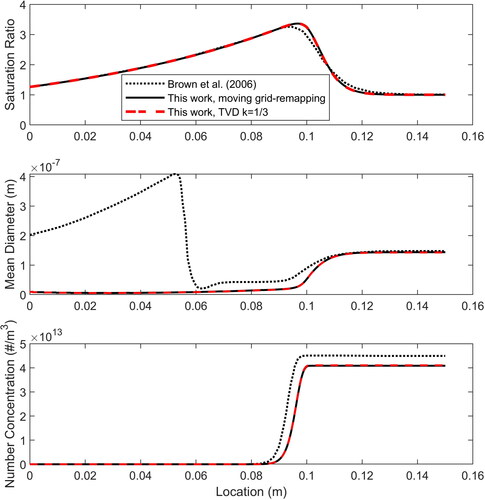
Figure 9 shows the calculated axial profiles for the saturation ratio, the mean particle diameter, and the total number concentration. As the gas is being cooled along the reactor, the saturation ratio is increasing due to the drop of vapor saturation pressure with temperature. When it exceeds a value around three, intense gas-to-particle conversion initiates and particles begin to form by homogeneous nucleation. Small increase in the saturation ratio further downstream causes the nucleation rate to increase rapidly creating the steep nucleation front showed by the sharp increase in particle number concentration at about 0.09 m. The newly formed particles then grow due to the condensation of CsOH vapor on their surface resulting to the increase of the particle mean diameter, as shown in the middle panel. Depletion of CsOH vapor by condensation causes the saturation ratio to decrease and eventually gas-to-particle conversion ceases. Indistinguishable results are also obtained using the TVD scheme for the solution of growth. In the figure, the results of Brown et al. (2006), who used a moment aerosol model, are also shown. We can observe that identical phenomenology is predicted by the two models in the nucleation-condensation zone. The differences in the prediction of the mean particle diameter (middle panel) upstream are considered trivial since they refer to a zone where negligible particle concentration exists, and they can be attributed to the different models used. In the moment model used in Brown et al. (2006) a log-normal distribution with a non-zero mean diameter is assumed everywhere, including in regions where particle formation is negligible. On the contrary, the present model calculates the mean particle diameter based on the actual particles predicted in each position. There are some small quantitative deviations between the two models in the nucleation zone also; in general, our calculations predict a slightly lower and delayed particle formation. The reasons for these small deviations have not been determined. It is likely, that they could be attributed to differences in the calculation of species properties that are not explicitly specified in Brown et al. (2006), such as vapor mean free path or vapor diffusion coefficient in the gas, or other differences in model and code setup, including the exact expression for the growth rate.

Figure 9. Axial variation of saturation ratio (up), geometrical mean particle diameter (middle) and particle number concentration (bottom), as calculated in the present work in comparison with the results of Brown et al. (2006), where a moment method was used.

So far, a fourth order Runge-Kutta method was used for the integration of the ODEs in each timestep. The TVD scheme was initially presented for the solution of growth using a simple explicit time stepping (Gunawan, Fusman, and Braatz 2004). Compared to using a robust e.g., Runge-Kutta solver, an explicit discretization might need smaller timesteps for achieving satisfactory accuracy. Moreover, to solve the system of the discretized TVD equations (Equation (5)(5) $$\frac{\partial n_i}{\partial t}+\frac{1}{\Delta d_i}\left({\left(Gn\right)}_{d_i^{+}}-{\left(Gn\right)}_{d_i^{-}}\right)=\frac{J\left(t\right)\delta (d-d_{\mathit{crit}})}{\Delta d_i}$$(5) ) explicitly in time (by a forward Euler time stepping method), the Courant-Friedrichs-Levy (CFL) condition must be met in the particle size dimension. This has been indicated also by Gunawan, Fusman, and Braatz (2004). The CFL criterion for the solution of growth can be written as: (24) $${\mathit{CFL}}_{i,j}=\mathrm{}\left|\frac{G_i\mathrm{}{\Delta t}_i}{\Delta d_j}\right|=|\frac{G_i\Delta x_i/u_{g,i}}{\Delta d_j}|<1$$(24) where, ${\Delta t}_i$ is the timestep corresponding to the axial step $\Delta x_i$ and $\Delta d_j$ the width of particle size bin $j.$ The CFL condition requires that the smaller is the time step the higher must be the number of particle size bins to ensure convergence. However, due to its lower computational cost per timestep, an explicit time discretization might be attractive in terms of the overall computational cost. So, in addition to the calculations using a Runge-Kutta method, we also examined this option by using an explicit time discretization in the nucleation-condensation problem described above. 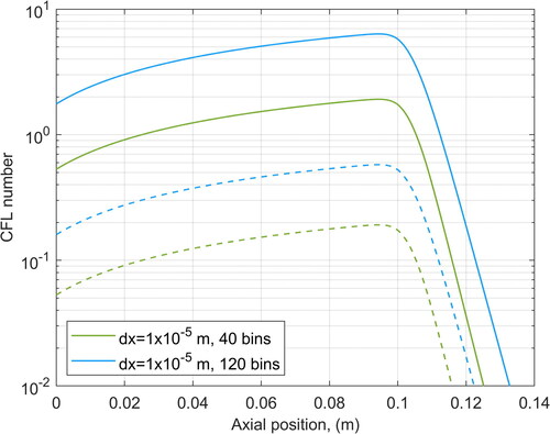In this case, for the TVD method, the system of Equation (5)(5) $$\frac{\partial n_i}{\partial t}+\frac{1}{\Delta d_i}\left({\left(Gn\right)}_{d_i^{+}}-{\left(Gn\right)}_{d_i^{-}}\right)=\frac{J\left(t\right)\delta (d-d_{\mathit{crit}})}{\Delta d_i}$$(5) is solved by an explicit (forward) Euler time stepping approach as in Gunawan, Fusman, and Braatz (2004). The calculations showed that very small axial steps are necessary to achieve stability and convergence. To explain this finding, in Figure 10 we present the maximum and average CFL number along the axial position for two particle size resolutions. As it is inferred, very low axial steps are necessary to satisfy the CFL criterion for all bins throughout the simulation. We must note that the TVD scheme solution may converge even when the maximum CFL is somewhat greater than unity. This means that although there may be some bins where the CFL criterion is violated, yet these bins do not necessarily affect the overall convergence. In our calculations, however, convergence with the TVD scheme was achieved only with very small axial steps. More specifically, convergence was achieved for axial steps of the order of or lower than $2.5\times {10}^{-5}\mathrm{}\mathrm{m}$ (corresponding to an about equal time step in seconds, taking into account that the gas velocity is about 1 m/s).

Figure 10. Evolution of the average (dash lines) and maximum (solid lines) value of CFL number for condensational growth along the axial direction, for two particle size resolutions.

This CFL restriction does not apply for the moving grid-remapping method. In this case, we only need to integrate the growth rate equation (Equation (7)(7) $${\mathit{dlm}}_i={\int }_0^{\Delta t}G\left(d\right)dt,\mathrm{}{d}_{t=0}={dl}_i,\mathrm{}i=1,\dots ,\mathit{nbin}+1$$(7) ) with a first order explicit discretization, which may reduce the accuracy in the prediction of the moved particle diameters during the moving grid step, but it does not affect the stability of the overall method. Using an explicit time stepping for the solution of the growth equation in the moving grid step-remapping method was found to be attractive due its very much lower computational cost. In Table 1, the computational time for representative simulations with TVD scheme and the moving grid-remapping method is provided. It should be noted that variation in the axial step results to a roughly proportional change in the computational time. It is apparent that the computational time required using an ODE solver is much higher compared to the explicit discretization. As it will be shown below, the accuracy of the overall calculations with the moving grid-remapping method is not significantly affected using an explicit time stepping. This provides the attractive potential that a simple explicit time stepping might be a feasible alternative in multidimensional cases also. We must stress, however, that this is a hypothesis that can be tested only in the context of CFD calculations. As it is inferred from Table 1, if an ODE solver is used for both methods, then the two methods require comparable time, which increase in a similar, linear trend with the number of bins. The moving grid-remapping method even though it requires additional loops for the remapping, yet presents a bit lower computational cost. This may be explained by the fact that only the non-zero bins are distributed back to the fixed grid, thus limiting the processing operations that are needed for the remapping step.

Table 1. Computational time (s) for the solution of the CsOH nucleation-condensation case for axial step size equal to ${10}^{-3}\mathrm{}\mathrm{m}.$

Number of bins	Moving grid- remapping		TVD, $k=1/3,\mathrm{}$ Qamar et al. (2006)
	Runge-Kutta	Explicit	Runge-Kutta
10	10	1	15
20	18	2	27
40	33	3	55
80	63	5	118
160	124	9	352

To further evaluate the performance of the methods, a sensitivity analysis regarding the effect of the number of particle size bins and the axial step was conducted. 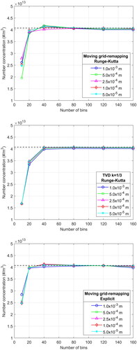Besides the moving grid-remapping method and the TVD scheme, calculations were also performed using the first-order discretization scheme of Equation (4)(4) $${\left.\frac{d{V}_i}{dt}\right|}_{\mathit{growth}}=G_{v,i-1}\frac{N_{i-1\mathrm{}}{v}_{i-1}}{v_i-v_{i-1}}-G_{v,i}\frac{N_i{v}_i}{v_{i+1}-v_i}$$(4) . Although not included in figures, the main findings using the first order scheme are also discussed. Figure 11 shows the calculated particle number concentration at the exit. For the moving grid-remapping method, results are presented using the fourth order Runge-Kutta method and the explicit time stepping. For the TVD scheme, results are presented only with the Runge-Kutta method since, as described above, convergence with an explicit time stepping was difficult to achieve. With the horizontal dot line, the solution using 320 bins and axial spatial step equal to 10⁻⁵ m is shown. The TVD scheme depicts a smooth behavior with increasing particle size and axial resolution, converging monotonically to the solution. The moving grid-remapping method presents some differences in its behavior, as it converges with small fluctuations around the solution. A particle size resolution of 40 bins, that is, less than 8 bins/decade is adequate to achieve a satisfactory accuracy in predicting the number concentration of the formed particles at the exit. The larger error for this number of bins is around 2.5% for both methods and decreases depending on the axial resolution, with the TVD method presenting a somehow higher accuracy. As it is observed, the moving grid-remapping method retains almost the same behavior and accuracy when an explicit time discretization is used instead of the most robust and accurate Runge-Kutta method. However, the computational time is one order of magnitude lower in this case (Table 1) or even more if compared with the TVD scheme. The first order discretization method showed very slow convergence, as several hundreds of particle size bins i.e., at least one order of magnitude more, were required to achieve a comparable level of accuracy. It is important to recall at this point, that in the context of CFD calculations the number of additional transport equations that must be solved in a sectional framework is equal to the number of particle size bins, so the extra computational cost with the first order scheme is expected to be much higher.

Figure 11. Total particle number concentration at the exit, as calculated with the moving grid - remapping method (top and bottom) and the TVD scheme (middle), for various particle size and axial space resolutions. The method used for the solution of the ODEs in each case is indicated in the legend.

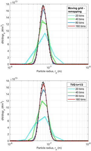
Finally, Figure 12 presents the distributions of CsOH particles sizes at the exit, as calculated by the moving grid-remapping method and the TVD scheme for different numbers of bins and axial step sizes. The solution using 320 bins and axial spatial step equal to 10⁻⁵ m is also shown. Both methods reproduce the sharp shape of the distribution and converge to the exact solution with the increase of the number of bins. To obtain a fine representation of the details of the distribution, however, a higher number of bins is required, compared to that needed for the prediction of the total number of particles. The error in prediction of the maximum value (peak) of the size distribution can be used as a simple indicator of the level of accuracy regarding the prediction of the distribution details. Calculations using the moving grid-remapping method and 80 bins (16 bins/decade) predict a maximum value which is 7% lower than the final solution. Using 160 bins (32 bins/decade) the deviation reduces to about 3%. The results also show a stable behavior with different axial steps, indicating that the number of computational iterations and the corresponding accumulated numerical errors do not significantly influence the prediction of the particle size distribution. A similar behavior is depicted in the case of the TVD scheme regarding its dependency on both the particle size and axial resolution. As in the previous pure condensation cases, the moving grid-remapping method shows a slightly better performance in combating numerical diffusion and representing the details of the distribution. The results of the moving grid-remapping method in Figure 12 refer to the case where the Runge-Kutta method is used. Almost identical results for the particle size distribution are obtained using the explicit time discretization, as it was also the case for the prediction of the number of particles, previously.

Figure 12. The exit size distribution of the formed CsOH particles, as calculated with the proposed method (top) and the TVD scheme (bottom) for different particle size and axial resolution (dash lines: $\mathrm{dx}={10}^{-3}\text{m}$ dot lines: $\mathrm{dx}=5·{10}^{-4}\mathrm{}\mathrm{m},$ solid lines: $\mathrm{dx}={10}^{-4}\mathrm{}\mathrm{m}$). The black line with markers represents the solution with 320 bins and $\mathrm{dx}={10}^{-5}\mathrm{}\mathrm{m}.$

Conclusions

In this work, a sectional method for the numerical solution of condensational growth was evaluated. The method is based on a two-step moving grid-remapping approach. During a timestep, the evolution of the distribution due to particle condensation or evaporation is, first, accurately predicted by numerical integration of the particle growth equation. At the second step, the particles of the moved bins are distributed back to the fixed grid. The main novelty of the method is related with the remapping of the moved distribution to the fixed grid. In the present method the particles of a moved bin are distributed to all fixed bins that the moved one crosses. Moreover, instead of a constant value, the particle distribution is assumed to varies linearly inside the moved bins. The slope inside a moved bin is evaluated based on the values of the size distribution at the adjacent bins, thus taking advantage of the actual shape of the moved distribution. Provided that the characteristic size of the particle size bins is defined at their center, the method inherently conserves the number of particles.

The method was compared with a high resolution TVD scheme for population balances. To provide a figure of the amount of numerical diffusion produced, calculations with a first order discretization scheme were also performed. The methods were initially tested against exact analytical and numerical solutions for the evolution of the size distribution due to condensation or evaporation. The condensation cases involved sharp unimodal and more complicated bi-modal distributions. The moving grid-remapping method was found to be stable and free of overshoots in all calculations performed. Both the present method and the TVD scheme were capable to cope with numerical diffusion efficiently. The two methods required a comparable particle size resolution to satisfactory reproduce the particle size distribution. It is worth noting that the first order scheme required a much- about one order of magnitude or more - finer size resolution to achieve a comparable level of accuracy.

The primary focus of this work was the evaluation of the method for cases dominated by intense gas-to-particle conversion through the competing processes of homogeneous nucleation and condensation. For this purpose, we used an aerosol flow case in a hypothetical one-dimensional aerosol reactor, which has previously been investigated in the literature. This case presents a strong, competing coupling between nucleation and condensation, largely different time scales between transport and aerosol dynamics, as well as a sharp final particle size distribution. Both the present moving grid-remapping method and the TVD scheme were able to cope with numerical diffusion, thus allowing for the adequate resolution of the coupling of the processes in the intense nucleation region. Regarding prediction of the number of the formed particles, the method converged to the particle size grid independent solution with less than 8 bins/decade. The deviation in the particle number prediction, varied slightly, depending on the axial step (or equivalently the timestep), but remained below about 2.5% even for the larger steps, for the moving grid-remapping method and the TVD scheme. The first order discretization scheme again required one order of magnitude finer particle size resolution, to approach the same accuracy in the prediction of the particle number. Regarding prediction of the particle size distribution, the two methods were able to reproduce its sharp shape, even though a higher number of size bins were required for an accurate prediction of the peak of the distribution. Indicatively, 20 bins/decade led to prediction of the peak of the distribution with about 7% deviation, while using a resolution of 40 bins/decade the difference dropped to about 3%.

The moving grid-remapping method and the TVD scheme can be used in multidimensional calculations in the context of a transient approach. This is not, however, a significant restriction because steady state cases can be easily treated in a pseudo-transient approach. It may be even preferable to solve complex problems with different time scales, as aerosol flows, in a transient context, since it allows selection of the most suitable solution for each process freely, and independently from the others. We believe that both methods can be helpful in extending the practical application and the efficiency of contemporary multi-purpose CFD codes in aerosol flow simulations. Using a Runge-Kutta ODE solver, both methods showed stability independently from the time discretization. In this way, the methods can be considered potentially attractive for multidimensional CFD calculations where the overall computational cost directly depends on the size of the time step. Moreover, the moving grid-remapping method is not subject to convergence conditions and can be used even with a simple explicit time discretization, with no stability restrictions regarding the magnitude of the timestep. Use of an explicit time stepping was found to reduce more than one order of magnitude the computational cost for the CsOH nucleation-condensation case, for the same level of accuracy. Therefore, it may be attractive as an alternative approach, and it may deserve further testing in the context of multidimensional CFD calculations.

Acknowledgments

We want to thank Prof. M. Yamamoto (Kyushu University, Japan) for his kind and helpful advice on calculation of the growth rate of sulfuric acid that we used for the validation of our model.

References

- Abarham, M., P. Zamankhan, J. W. Hoard, D. Styles, C. Scott Sluder, J. M. E. Storey, M. J. Lance, and D. Assanis. 2013. CFD analysis of particle transport in axi-symmetric tube flows under the influence of thermophoretic force. Int. J. Heat Mass Transf. 61 (1):94–105. doi: 10.1016/j.ijheatmasstransfer.2013.01.071.
- Alopaeus, V., M. Laakkonen, and J. Aittamaa. 2006. Numerical solution of moment-transformed population balance equation with fixed quadrature points. Chem. Eng. Sci. 61 (15):4919–29. doi: 10.1016/j.ces.2006.03.028.
- Ansys, Inc. 2019. Ansys FLUENT 19.2. Theory Guide. Canonsburg, PA: Ansys, Inc.
- Bouaniche, A., L. Vervisch, and P. Domingo. 2019. A hybrid stochastic/fixed-sectional method for solving the population balance equation. Chem. Eng. Sci. 209:115198. doi: 10.1016/j.ces.2019.115198.
- Bouaniche, A., J. Yon, P. Domingo, and L. Vervisch. 2020. Analysis of the soot particle size distribution in a laminar premixed flame: A hybrid stochastic/fixed‑sectional approach. Flow Turbulence Combust. 104 (2–3):753–75. doi: 10.1007/s10494-019-00103-2.
- Brown, D. P., E. I. Kauppinen, J. K. Jokiniemi, S. G. Rubin, and P. Biswas. 2006. A method of moments based CFD model for polydisperse aerosol flows with strong interphase mass and heat transfer. Comput. Fluids 35 (7):762–80. doi: 10.1016/j.compfluid.2006.01.012.
- di Veroli, G. Y., and S. Rigopoulos. 2011. Modeling of aerosol formation in a turbulent jet with the transported population balance equation-probability density function approach. Phys. Fluids 23 (4):043305. doi: 10.1063/1.3576913.
- Drossinos, Y., and N. I. Stilianakis. 2020. What aerosol physics tells us about airborne pathogen transmission. Aerosol Sci. Technol. 54 (6):639–43. doi: 10.1080/02786826.2020.1751055.
- Frederix, E. M. A., A. K. Kuczaj, M. Nordlund, A. E. P. Veldman, and B. J. Geurts. 2017. Application of the characteristics-based sectional method to spatially varying aerosol formation and transport. J. Aerosol Sci. 104:123–40. doi: 10.1016/j.jaerosci.2016.10.008.
- Frenkel, J. 1955. Kinetic theory of liquids. New York: Dover Publications.
- Friedlander, S. K. 2000. Smoke, dust, and haze – Fundamentals of aerosol dynamics. 2nd ed. New York: Oxford University Press.
- Garcia, M., L. E. Herranz, and M. P. Kissane. 2016. Theoretical assessment of particle generation from sodium pool fires. Nucl. Eng. Des. 310:470–83. doi: 10.1016/j.nucengdes.2016.10.024.
- Gelbard, F., Y. Tambour, and J. H. Seinfeld. 1980. Sectional representations for simulating aerosol dynamics. J. Colloid Interface Sci. 76 (2):541–56. doi: 10.1016/0021-9797(80)90394-X.
- Girshick, S. L., and C. P. Chiu. 1990. Kinetic nucleation theory: A new expression for the rate of homogeneous nucleation from an ideal supersaturated vapor. J. Chem. Phys. 93 (2):1273–7. doi: 10.1063/1.459191.
- Gunawan, R., I. Fusman, and R. D. Braatz. 2004. High resolution algorithms for multidimensional population balance equations. AIChE J. 50 (11):2738–49. doi: 10.1002/aic.10228.
- Herranz, L. E., M. Garcia, M. P. Kissane, and C. Spengler. 2018. A lumped parameter modelling of particle generation from Na-pool fires in SFR containments. Prog. Nucl. Energy 109:223–32. doi: 10.1016/j.pnucene.2018.08.015.
- Hinds, W. C. 2012. Aerosol technology: Properties, behavior, and measurement of airborne particles. 2nd ed. New York: John Wiley & Sons.
- Hounslow, M. J., R. L. Ryall, and V. R. Marshall. 1988. A discretized population balance for nucleation, growth, and aggregation. AIChE J. 34 (11):1821–32. doi: 10.1002/aic.690341108.
- Jacobson, M. Z. 1997. Development and application of a new air pollution modelling system-II. aerosol module structure and design. Atmos. Environ. 31 (2):131–44. doi: 10.1016/1352-2310(96)00202-6.
- Jokiniemi, J. K., M. Lazaridis, K. E. J. Lehtinen, and E. I. Kauppinen. 1994. Numerical simulation of vapor-aerosol dynamics in combustion processes. J. Aerosol Sci. 25 (3):429–46. doi: 10.1016/0021-8502(94)90062-0.
- Kim, Y. P., and J. H. Seinfeld. 1990. Simulation of multicomponent aerosol condensation by the moving sectional method. J. Colloid Interface Sci. 135 (1):185–99. doi: 10.1016/0021-9797(90)90299-4.
- Kissane, M. P., D. Mitrakos, C. Housiadas, and J. C. Sabroux. 2009. Investigation of thermo-catalytic decomposition of metal-iodide aerosols due to passage through hydrogen recombiners. Nucl. Eng. Des. 239 (12):3003–13. doi: 10.1016/j.nucengdes.2009.08.001.
- Kumar, S., and D. Ramkrishna. 1996a. On the solution of population balance equations by discretization –I. A fixed pivot technique. Chem. Eng. Sci. 51 (8):1311–32. doi: 10.1016/0009-2509(96)88489-2.
- Kumar, S., and D. Ramkrishna. 1996b. On the solution of population balance equations by discretization – II. A moving pivot technique. Chem. Eng. Sci. 51 (8):1333–42. doi: 10.1016/0009-2509(95)00355-X.
- Kumar, S., and D. Ramkrishna. 1997. On the solution of population balance equations by discretization – III. Nucleation, growth and aggregation of particles. Chem. Eng. Sci. 52 (24):4659–79. [Database] doi: 10.1016/S0009-2509(97)00307-2.
- Lee, J., K. S. Ha, and J. Hwang. 2017. Application of moment method for predicting condensational growth of nuclear aerosols in a severe accident. Nucl. Technol. 200 (3):241–9. doi: 10.1080/00295450.2017.1372984.
- Lee, Y., Y. J. Cho, and K. Lim. 2019. Coupling scheme of multicomponent sectional equations and Mason equations via transition rate matrix of hygroscopic growth applied to international standard problem No. 44. Ann. Nucl. Energy 127:437–49. doi: 10.1016/j.anucene.2018.12.028.
- Liu, A., and S. Rigopoulos. 2019. A conservative method for numerical solution of the population balance equation, and application to soot formation. Combust. Flame 205:506–21. doi: 10.1016/j.combustflame.2019.04.019.
- Lurmann, F. W., A. S. Wexler, S. N. Pandis, S. Musarra, N. Kumar, and J. H. Seinfeld. 1997. Modelling urban and regional aerosols-II. Application to California’s south coast air basin. Atmos. Environ. 31 (17):2695–715. doi: 10.1016/S1352-2310(97)00100-3.
- Mahrukh, M., A. Kumar, S. Gu, and S. Kamnis. 2016. Computational development of a novel aerosol synthesis technique for production of dense and nanostructured zirconia coating. Ind. Eng. Chem. Res. 55 (28):7679–95. doi: 10.1021/acs.iecr.6b01725.
- Marchisio, D. L., and R. O. Fox. 2005. Solution of population balance equations using the direct quadrature method of moments. J. Aerosol Sci. 36 (1):43–73. doi: 10.1016/j.jaerosci.2004.07.009.
- Marchisio, D. L., R. D. Vigil, and R. O. Fox. 2003. Implementation of the quadrature method of moments in CFD codes for aggregation – Breakage problems. Chem. Eng. Sci. 58 (15):3337–51. doi: 10.1016/S0009-2509(03)00211-2.
- Mason, B. J. 1971. The Physics of Clouds. Oxford: Clarendon Press.
- McGraw, R. 1997. Description of aerosol dynamics by the quadrature method of moments. Aerosol Sci. Technol. 27 (2):255–65. doi: 10.1080/02786829708965471.
- McGraw, R., and D. L. Wright. 2003. Chemically resolved aerosol dynamics for internal mixtures by the quadrature method of moments. Aerosol Sci. 34 (2):189–209. doi: 10.1016/S0021-8502(02)00157-X.
- Mitrakos, D., J. Jokiniemi, U. Backman, and C. Housiadas. 2008. Aerosol flow in a tube furnace reactor of gas-phase synthesised silver nanoparticles. J. Nanopart. Res. 10 (S1):153–61. doi: 10.1007/s11051-008-9439-3.
- Mitrakos, D., E. Hinis, and C. Housiadas. 2007. Sectional modeling of aerosol dynamics in multi-dimensional flows. Aerosol Sci. Technol. 41 (12):1076–88. doi: 10.1080/02786820701697804.
- Mitsakou, C., C. Helmis, and C. Housiadas. 2004. Extrathoracic and thoracic deposition of inhaled hygroscopic particles. J. Aerosol. Sci. 35 (S2):S1127–S1128. doi: 10.1016/s0021-8502(19)30296-4.
- Mohs, A. J., and F. M. Bowman. 2011. Eliminating numerical artifacts when presenting moving center sectional aerosol size distributions. Aerosol Air Qual. Res. 11 (1):21–30. doi: 10.4209/aaqr.2010.06.0046.
- Netz, R. 2020. Mechanisms of airborne infection via evaporating and sedimenting droplets produced by speaking. J. Phys. Chem. B. 124 (33):7093–101. doi: 10.1021/acs.jpcb.0c05229.
- Park, S. H., and S. N. Rogak. 2004. A novel fixed-sectional model for the formation and growth of aerosol agglomerates. J. Aerosol Sci. 35 (11):1385–404. doi: 10.1016/j.jaerosci.2004.05.010.
- Pilou, M., V. Antonopoulos, E. Makris, P. Neofytou, S. Tsangaris, and C. Housiadas. 2013. A fully Eulerian approach to particle inertial deposition in a physiologically realistic bifurcation. Appl. Math. Modell. 37 (8):5591–605. doi: 10.1016/j.apm.2012.10.055.
- Pratsinis, S. E. 1988. Simultaneous nucleation, condensation, and coagulation in aerosol reactors. J. Colloid Interface Sci. 124 (2):416–27. doi: 10.1016/0021-9797(88)90180-4.
- Pyykönen, J., J. Enriquez, D. Brown, and J. K. Jokiniemi. 2002. Exploring the limits of the sectional approach in the CFD based simulation of aerosol dynamics. In 6th International Aerosol Conference, International Aerosol Research Assembly, 569–570.
- Pyykönen, J., and J. Jokiniemi. 2000. Computational fluid dynamics based sectional aerosol modelling schemes. J. Aerosol Sci. 31 (5):531–50. doi: 10.1016/S0021-8502(99)00546-7.
- Qamar, S., M. P. Elsner, I. A. Angelov, G. Warnecke, and A. Seidel-Morgenstern. 2006. A comparative study of high resolution schemes for solving population balances in crystallization. Comput. Chem. Eng. 30 (6–7):1119–31. doi: 10.1016/j.compchemeng.2006.02.012.
- Qamar, S., A. Ashfaq, G. Warnecke, I. Angelov, M. P. Elsner, and A. Seidel-Morgenster. 2007. Adaptive high-resolution schemes for multidimensional population balances in crystallization processes. Comput. Chem. Eng. 31 (10):1296–311. doi: 10.1016/j.compchemeng.2006.10.014.
- Ramkrishna, D. 2000. Population balances: Theory and applications to particulate systems in engineering. Cambridge, MA: Academic Press.
- Roussos, A. I., A. H. Alexopoulos, and C. Kiparissides. 2006. Dynamic evolution of PSD in continuous flow processes: A comparative study of fixed and moving grid numerical techniques. Chem. Eng. Sci. 61 (1):124–34. doi: 10.1016/j.ces.2004.12.056.
- Rosner, D. E., and J. Pyykonen. 2002. Bivariate moment simulation of coagulating and sintering nanoparticles in flames. AIChE J. 48 (3):476–91. doi: 10.1002/aic.690480307.
- Schwade, B., and P. Roth. 2003. Simulation of nano-particle formation in a wall-heated aerosol reactor including coalescence. J. Aerosol Sci. 34 (3):339–57. doi: 10.1016/S0021-8502(02)00186-6.
- Seigneur, C., A. B. Hudischewskyj, J. H. Seinfeld, K. T. Whitby, E. R. Whitby, J. R. Brock, and H. M. Barnes. 1986. Simulation of aerosol dynamics: A comparative review of mathematical models. Aerosol Sci. Technol. 5 (2):205–22. doi: 10.1080/02786828608959088.
- Seinfeld, J. H., and S. N. Pandis. 2006. Atmospheric chemistry and physics: From air pollution to climate change. 2nd ed. New Jersey: Wiley-Interscience.
- Sewerin, F., and S. Rigopoulos. 2017a. An LES-PBE-PDF approach for modeling particle formation in turbulent reacting flows. Phys. Fluids 29 (10):105105. doi: 10.1063/1.5001343.
- Sewerin, F., and S. Rigopoulos. 2017b. An explicit adaptive grid approach for the numerical solution of the population balance equation. Chem. Eng. Sci. 168:250–70. doi: 10.1016/j.ces.2017.01.054.
- Shiea, M., A. Buffo, M. Vanni, and D. Marchisio. 2020. Numerical methods for the solution of population balance equations coupled with computational fluid dynamics. Annu. Rev. Chem. Biomol. Eng. 11 (1):339–66. doi: 10.1146/annurev-chembioeng.
- Singh, S.,. P. J. Adams, A. Misquitta, K. J. Lee, E. M. Lipsky, and A. L. Robinson. 2014. Computational analysis of particle nucleation in dilution tunnels: Effects of flow configuration and tunnel geometry. Aerosol Sci. Technol. 48 (6):638–48. doi: 10.1080/02786826.2014.910291.
- Stratmann, F., and E. R. Whitby. 1989. Numerical solution of aerosol dynamics for simultaneous convection, diffusion and external forces. J. Aerosol Sci. 20 (4):437–40. doi: 10.1016/0021-8502(89)90077-3.
- Tang, H., and T. Tang. 2003. Adaptive mesh methods for one- and two-dimensional hyperbolic conservation laws. SIAM J. Numer. Anal. 41 (2):487–515. doi: 10.1137/S003614290138437X.
- Tang, T. 2005. Moving mesh methods for computational fluid dynamics. In Contemporary mathematics, 383. Proceedings of the International Conference on Recent Advances in Adaptive Computation, May 24–28, 2004, Zhejiang University, Hangzhou, China. Rhode Island: American Mathematical Society.
- Wilck, M., and F. Stratmann. 1997. A 2-D multicomponent modal aerosol model and its application to laminar flow reactors. J. Aerosol Sci. 28 (6):959–72. doi: 10.1016/S0021-8502(96)00481-8.
- Woo, M., R. T. Nishida, M. A. Schriefl, M. E. J. Stettler, and A. M. Boies. 2021. Open-source modelling of aerosol dynamics and computational fluid dynamics: nodal method for nucleation, coagulation, and surface growth. Comput. Phys. Commun. 261:107765. doi: 10.17632/3s368jpdx2.1.
- Yamamoto, M. 2004. A solver for aerosol condensation equation by semi-Lagrangian scheme with correction exactly conserving total particle number. Aerosol Sci. Technol. 38 (10):1033–43. doi: 10.1080/027868290524025.
- Yamamoto, M. 2012. Numerical error analysis of solvers using cumulative number distribution with volume-ratio grid spacing in initially particle-free nucleation-condensation systems. Aerosol Air Qual. Res. 12 (6):1125–34. doi: 10.4209/aaqr.2012.02.0042.
- Zhang, Y., C. Seigneur, J. H. Seinfeld, M. Z. Jacobson, and F. S. Binkowski. 1999. Simulation of aerosol dynamics: A comparative review of algorithms used in air quality models. Aerosol Sci. Technol. 31 (6):487–514. doi: 10.1080/027868299304039.
- Zhao, B., C. Chen, and Z. Tan. 2009. Modeling of ultrafine particle dispersion in indoor environments with an improved drift flux model. J. Aerosol Sci. 40 (1):29–43. doi: 10.1016/j.jaerosci.2008.09.001.