Fundamentals of low-cost aerosol sensor design and operation

Abstract

Most evaluations of low-cost aerosol sensors have focused on their measurement bias compared to regulatory monitors. Few evaluations have applied fundamental principles of aerosol science to increase our understanding of how such sensors work and could be improved. We examined the Plantower PMS5003 sensor’s internal geometry, laser properties, photodiode responses, microprocessor output, flow rates, and response to mono- and poly-disperse aerosols. We developed a physics-based model of particle light scattering within the sensor, which we used to predict counting and sizing efficiency for 0.30 to 10 µm particles. We found that the PMS5003 counts single particle scattering events, acting like an imperfect optical particle counter, rather than a nephelometer. As particle flow is not focused into the core of the laser beam, >99% of particles that flow through the PMS5003 miss the laser, and those that intercept the laser usually miss the focal point and are subsequently undersized, resulting in erroneous size distribution data. Our model predictions of PMS5003 response to varying particle diameters, aerosol compositions, and relative humidity were consistent with laboratory data. Computational fluid dynamics simulations of the PurpleAir monitor housing showed that for wind-speeds less than 3 m s⁻¹, fine and coarse particles were representatively aspired to the PMS5003 inlet. Our measurements and models explain why the PurpleAir overstates regulatory PM_2.5 in some locations but not others; why the PurpleAir PM₁₀ is unresponsive to windblown dust; and why it reports a similar particle size distribution for coarse particles as it does for smoke and ambient background aerosol.

Copyright © 2023 American Association for Aerosol Research

EDITOR:

• Jonathan P. Reid

1. Introduction

The use of low-cost sensors for particulate matter (PM) air pollution has grown dramatically over the last decade—driven by their low cost, small size, low power consumption, and portability (Solomon and Dhaniyala 2020). For example, as of December 2022, there were approximately 30,000 PurpleAir monitors online (Tengono 2022). The majority of these PurpleAir monitors utilize the Plantower PMS5003 sensor, which is arguably the most common low-cost PM sensor in use today (Molina Rueda et al. 2023). Low-cost PM sensors are used in a variety of applications, such as tracking wildfire smoke plumes (“Fire and Smoke Map” 2023), identifying “hot spots” and estimating impact on vulnerable populations (Cheeseman et al. 2022; Nguyen et al. 2021; Sun et al. 2022); assessing personal exposure (Do et al. 2021; Fanti et al. 2021); estimating global aerosol impacts and improving global climate modeling (Bittner et al. 2022; Dhammapala et al. 2022; Glib et al. 2021; Snider et al. 2015); as well as making aerial measurements by drone, aircraft, or balloon (Chen et al. 2022; Dubey, Patra, and Nazneen 2022; Pharis et al. 2022; Pang et al. 2021).

Most low-cost PM sensors use light scattering to estimate aerosol mass concentration. In many recent studies, these low-cost sensors have been evaluated or “calibrated” by comparing their measurements with those from regulatory- and research-grade instruments. For example, researchers have found that the PurpleAir tends to overestimate regulatory PM_2.5 in the USA (Barkjohn, Gantt, and Clements 2021) but not in Beijing (Mei et al. 2020). This sensor also tends to overestimate regulatory PM_2.5 with increasing relative humidity (RH), but not as rapidly as hygroscopic growth theory would predict (Barkjohn, Gantt, and Clements 2021; Tryner et al. 2020a). The PurpleAir severely underestimates regulatory PM_2.5 and PM₁₀ concentrations during wind-blown dust episodes (Molina Rueda et al. 2023; Kaur and Kelly 2023a; Jaffe et al. 2023). Published performance evaluations have helped users understand and potentially reduce the measurement bias and uncertainty from the PurpleAir and other monitors (Barkjohn, Gantt, and Clements 2021; Hofman et al. 2022; Jain, Presto, and Zimmerman 2021; Lee, Wang, and Yu 2019; Malings et al. 2020; Levy Zamora et al. 2023); however, few have applied aerosol science and engineering principles to increase our understanding of how these sensors work and how they can be improved.

Many laboratory and field evaluations of PMS5003 response to aerosols (He, Kuerbanjiang, and Dhaniyala 2020; Ouimette et al. 2022) have concluded that the sensor behaves like a nephelometer, responding to an ensemble of particles rather than counting and sizing individual particles; yet, these sensors report particle size distribution data, which is more typical of an optical particle counter. Resolving this discrepancy requires us to evaluate the sensor response by probing the output of the photodiode directly.

In this study, the PMS5003 (1)(1) $$w\left(z\right)=w_0{\left(1+{\left(\frac{z}{z_0}\right)}^2\right)}^{0.5}$$(1) laser beam profile, (2)(2) $$I_{\max }=\mathrm{ }\frac{P}{0.5\pi w_o^2}$$(2) photodiode output, and (3)(3) $$I_p(x,y,z)=\frac{P}{0.5\mathrm{ }\pi w_0^2}\mathrm{ }\frac{1}{1+{\left(z/z_0\right)}^2}\mathrm{ }\exp \left[\frac{-2{\left(r/w_0\right)}^2}{1+{\left(z/z_0\right)}^2}\right]$$(3) flowrate, as well as (4)(4) $$I=I_p\frac{\left({\left|S_1\left(\theta \right)\right|}^2{\cos }^2\left(\varphi \right)+{\left|S_2\left(\theta \right)\right|}^2{\sin }^2\left(\varphi \right)\right)\cos \hspace{0.17em}\left(\alpha \right)}{{\mathrm{k}}^2{d}^2}$$(4) the PMS5003 response to 0.10- and 0.20-µm polystyrene latex (PSL) aerosol were all measured. A physical-optical model of particle light scattering was used to predict the photodiode signal resulting from particle interaction with the focused Gaussian laser beam. The model was used to estimate particle counting efficiency and size attribution for 0.30- to 10-µm particles. Additionally, predictions from this model were compared to previously-published data on PMS5003 sensor performance in laboratory settings (Tryner et al. 2020a; Kaur and Kelly 2023b)—specifically, data on how the sensor responds to aerosols with varying size distributions and to changes in ambient RH. As these sensors are typically deployed with a housing in monitors such as the PurpleAir, we used computational fluid dynamics (CFD) simulations to determine the aspiration efficiency of PMS5003 sensor inside the PurpleAir housing.

These measurements, model, and analyses were designed to answer the following questions about the Plantower PMS5003 sensor: (1)(1) $$w\left(z\right)=w_0{\left(1+{\left(\frac{z}{z_0}\right)}^2\right)}^{0.5}$$(1) Does the PMS5003 function more like a nephelometer or an optical particle counter (OPC); (2)(2) $$I_{\max }=\mathrm{ }\frac{P}{0.5\pi w_o^2}$$(2) How do the sensor’s fan, laser, photodiode, and microprocessor interact and impact the sensor’s ability to estimate particle size distributions and mass concentrations; (3)(3) $$I_p(x,y,z)=\frac{P}{0.5\mathrm{ }\pi w_0^2}\mathrm{ }\frac{1}{1+{\left(z/z_0\right)}^2}\mathrm{ }\exp \left[\frac{-2{\left(r/w_0\right)}^2}{1+{\left(z/z_0\right)}^2}\right]$$(3) Does our physical-optical model predict PMS5003 response consistent with controlled laboratory studies; (4)(4) $$I=I_p\frac{\left({\left|S_1\left(\theta \right)\right|}^2{\cos }^2\left(\varphi \right)+{\left|S_2\left(\theta \right)\right|}^2{\sin }^2\left(\varphi \right)\right)\cos \hspace{0.17em}\left(\alpha \right)}{{\mathrm{k}}^2{d}^2}$$(4) Why does the PurpleAir overstate regulatory PM_2.5 in some locations but not others, (5)(5) $$k=2\pi /\lambda$$(5) How does the PMS5003 respond to increased RH; (6)(6) $$d={\left[{\left(x_p-x_d\right)}^2+{\left(y_p-y_d\right)}^2+{\left(z_p-z_d\right)}^2\right]}^{0.5}$$(6) Why is the PMS5003 unresponsive to coarse particles; (7)(7) $$d_1=z_p+4\mathrm{ }\mathrm{mm}$$(7) Why does the PMS5003 report a similar particle size distribution for coarse particles as it does for smoke and ambient background aerosols; and (8)(8) $$d_2={\left[{\left(x_p-x_d\right)}^2+{\left(y_p-y_d\right)}^2+{\left(z_d+4\right)}^2\right]}^{0.5}$$(8) What does the aspiration model predict about the PurpleAir response as a function of wind speed?

2. Materials and methods

Aerosol number and mass concentrations reported by the Plantower PMS5003 depend on many aspects of the sensor’s design, including the internal geometry, focused laser properties, photodiode, air flow rate, particle aspiration and transmission efficiency (between the inlet and particle sensing zone), and the proprietary signal processing algorithms used by its microprocessor. This section describes the measurements and models that were used to understand the fundamentals of the PMS5003 design and operation.

2.1. Laser beam profile measurements

Inside the PMS5003, the beam from the laser diode passes through a 3-mm diameter lens and then three 2.0-mm-diameter apertures (see Figure S1). The apertures transform the original elliptical cross section into an approximately circular cross section. The wavelength and power of three PMS5003 diode lasers were measured previously by Ouimette et al. (2022) using an Ocean Optics Red Tide USB650 spectrometer and Melles Griot Universal Optical Power Meter, respectively. In the present study, the diameter of the laser beam at and near its focal point was measured for two PMS5003 laser diodes using a dial gauge and beam profiler (ThorLabs WM100; which uses the “knife edge” technique). The beam profiler was then used to measure the beam radius in the direction parallel to polarization as a function of distance from the focal point. These measurements were made on two PMS5003 lasers that had not passed through the three 2.0-mm-diameter apertures due to physical limitations. The resulting data were compared to the Gaussian equation for beam radius w(z) (Moosmuller and She 1991): (1) $$w\left(z\right)=w_0{\left(1+{\left(\frac{z}{z_0}\right)}^2\right)}^{0.5}$$(1) with the laser propagating in the z direction and z = 0 at the focal point. The radial and longitudinal scaling parameters are the beam spot radius at the focal point, $w_0,$ and the Rayleigh length (z₀ = aw₀²/2), where a is a constant. The methods used to measure w₀ and z₀ are described in greater detail in Supplemental Information (SI) Section S2.1.

The peak intensity of the PMS5003 laser beam, I_max (W cm⁻²), at the focal point was then calculated as (Moosmuller and She 1991): (2) $$I_{\max }=\mathrm{ }\frac{P}{0.5\pi w_o^2}$$(2) where P was the power (W) measured by Ouimette et al. (2022).

2.2. Photodiode output measurements

Ouimette et al. (2022) inspected the PMS5003 printed circuit board visually and suggested that the sensor uses a Vishay VBPW34S photodiode. The photodiode current is processed by a Cypress Programmable System-On-Chip 4200 microprocessor. In the present study, we investigated whether the PMS5003 could detect individual particles by using a PC oscilloscope (PicoScope 6 – PC Oscilloscope software version 6.14.61.6219) to record and decode the analog photodiode output along with the standard PMS5003 serial output (i.e., aerosol number and mass concentrations) for each 1-s laser cycle (see SI Section 2.2 for additional details).

While the PMS5003 was connected to the oscilloscope, smoke was generated by combusting a match near the PMS5003 sample inlet. The smoke concentration was not controlled; it decreased when the match went out. During this test, 47 complete data samples were recorded from the PMS5003 over the course of one minute. Each sample consisted of 600 ms of analog data sent to the microprocessor and the processed data from the microprocessor. To determine the effectiveness of the PMS5003 in detecting and sizing individual particles in the smoke, detailed analyses were performed on two of the 47 samples: Sample 7 and Sample 31.

2.3. Flow rate measurement and effect of flow impedance on reported particle concentrations

The PMS5003 uses a miniature fan to draw air through it, which can pose difficulty for flow management and measurement. If the flow rate through the PMS5003 drops below the manufacturer-assumed value, the reported particle concentrations might change. The PMS5003 flow rate is not actively controlled; it is determined by the sensor’s internal flow impedance and the fan’s performance curve (i.e., a plot of the fan’s flow rate vs. static pressure (Goodfellow and Kosonen 2020)). The fan’s maximum static pressure at no flow is an important measure of how the PMS5003 will respond to upstream pressure changes due to wind, an additional housing placed around the sensor, or a sample pretreatment device placed upstream of the sensor. Additionally, the flow impedance imposed by traditional flow rate measurement devices might alter the flow rate through the sensor substantially, resulting in an incorrect low measurement.

We modified two PMS5003 sensors with pressure taps and fittings to measure the fan’s maximum static pressure. We also investigated how the PMS5003-reported concentration of particles larger than 0.3 µm (a metric we refer to as the “CH1” output) varied as a function of upstream pressure changes. Upstream pressure was varied by impeding the flow to the PMS5003 inlet through orifices varying from 0.50 to 5.9 mm diameter. Differential pressure was measured with a MAGRFHELIC TE-2000, 0–30 Pa gauge. Additionally, the flow rate through the sensor was measured with a TSI Model 4143 Mass Flowmeter installed at the inlet. Additional details on these experimental methods are in SI Section 2.3.

2.4. Estimating the PMS5003 particle size detection limit with polystyrene latex spheres

Plantower advertises the particle detection limit of the PMS5003 to be 0.3 µm. This limit was tested by placing eight PMS5003 sensors inside a laboratory aerosol chamber and exposing the sensors to aerosolized PSL spheres. The PSL spheres were suspended in LCMS-grade water and aerosolized using a Collison nebulizer. The aerosol output by the nebulizer was then passed through an electrostatic classifier (TSI Model 3082) before entering the chamber containing the PMS5003 sensors. The size distribution of the aerosol inside the chamber was monitored using a scanning mobility particle sizer (SMPS; TSI Model 3082 Electrostatic Classifier and TSI Model 3787 Condensation Particle Counter). This experiment was repeated twice: first with 0.2 µm PSL and then with 0.1 µm PSL. Data from the PMS5003 sensors—including particle number counts and mass distributions—were logged to a text file at 3-s intervals. See SI Section 2.4 and Figure S12 for additional details on the methods associated with this experiment.

2.5. Physical-optical particle light scattering model and computer program

Conventional (i.e., research- and regulatory-grade) optical particle counters (OPCs) typically direct sampled air into a small sensing volume where all particles are irradiated with the same intensity of light. As a result, there is usually a one-to-one relationship between photodiode voltage and a spherical particle diameter of known refractive index. This is not the case for the PMS5003; the sensor geometry does not force particles flowing through the region above the photodiode to pass through a single point within the laser beam. Consequently, even if the PMS5003 detects and counts individual particles, like an OPC, we would not expect it to respond to particles of varying diameters and refractive indices in the same manner as a conventional OPC. To investigate further, we developed a physical-optical model and a computer program, called “PA-PMS,” to simulate the PMS5003 response to single-particle light scattering events.

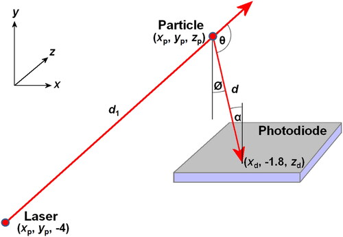
In our model’s coordinate system, the laser beam propagates in the z direction, particles flow in the x direction, and the y-axis is perpendicular to the photodiode (Figure 1). Laser beam propagation and particle flow are both parallel to the photodiode but perpendicular to each other. The origin—(x, y, z) = (0,0,0)—is defined as the focal point of the laser beam, which was found to be 1.8 mm directly above the center of the photodiode. Light from the laser beam is scattered by a single spherical particle of diameter D_p and refractive index m located at (x_p, y_p, z_p). The scattering plane is defined by the laser forward direction z and the ray from the particle to a point on the photodiode.

Figure 1. Schematic of the scattering process within the PMS5003. d₁ is the distance from the laser to the particle, d is the distance from the particle to the photodiode, θ is the scattering angle, ϕ is the angle of the scattering plane relative to the vertical, and α is the ray’s angle of arrival relative to the orthogonal of the photodiode.

The intensity of the laser beam, I_p (W cm⁻²), incident on a particle at point (x_p, y_p, z_p) in the PMS5003 transport channel is calculated using the Gaussian model (Moosmuller and She 1991): (3) $$I_p(x,y,z)=\frac{P}{0.5\mathrm{ }\pi w_0^2}\mathrm{ }\frac{1}{1+{\left(z/z_0\right)}^2}\mathrm{ }\exp \left[\frac{-2{\left(r/w_0\right)}^2}{1+{\left(z/z_0\right)}^2}\right]$$(3) where r = (x² + y²)^0.5.

The particle at (x_p, y_p, z_p) scatters light to the photodiode, and the intensity, I (W cm⁻²), of the scattered light at an arbitrary point (x_d, y_d, z_d) on the surface of the photodiode is calculated using Equation (4)(4) $$I=I_p\frac{\left({\left|S_1\left(\theta \right)\right|}^2{\cos }^2\left(\varphi \right)+{\left|S_2\left(\theta \right)\right|}^2{\sin }^2\left(\varphi \right)\right)\cos \hspace{0.17em}\left(\alpha \right)}{{\mathrm{k}}^2{d}^2}$$(4) : (4) $$I=I_p\frac{\left({\left|S_1\left(\theta \right)\right|}^2{\cos }^2\left(\varphi \right)+{\left|S_2\left(\theta \right)\right|}^2{\sin }^2\left(\varphi \right)\right)\cos \hspace{0.17em}\left(\alpha \right)}{{\mathrm{k}}^2{d}^2}$$(4) where S₁(θ) and S₂(θ) are the amplitude scattering functions for perpendicular and parallel polarization, respectively, at a scattering angle θ. S₁(θ) and S₂(θ) are functions of the scattering angle (θ), particle diameter (D_p), particle refractive index (m), and laser wavelength (λ). In Equation (4)(4) $$I=I_p\frac{\left({\left|S_1\left(\theta \right)\right|}^2{\cos }^2\left(\varphi \right)+{\left|S_2\left(\theta \right)\right|}^2{\sin }^2\left(\varphi \right)\right)\cos \hspace{0.17em}\left(\alpha \right)}{{\mathrm{k}}^2{d}^2}$$(4) , k is the wavenumber, d is the distance from the particle to the photodiode, ϕ is the angle of the scattering plane relative to the vertical, and α is the ray’s angle of arrival relative to the orthogonal of the photodiode. These values are calculated as shown in Equations (5)–(11)(11) $$\tan \hspace{0.17em}\left(\alpha \right)={\left[{\left(x_p-x_d\right)}^2+{\left(z_p-z_d\right)}^2\right]}^{0.5}/\left(y_p-y_d\right)$$(11) . (5) $$k=2\pi /\lambda$$(5) (6) $$d={\left[{\left(x_p-x_d\right)}^2+{\left(y_p-y_d\right)}^2+{\left(z_p-z_d\right)}^2\right]}^{0.5}$$(6) (7) $$d_1=z_p+4\mathrm{ }\mathrm{mm}$$(7) (8) $$d_2={\left[{\left(x_p-x_d\right)}^2+{\left(y_p-y_d\right)}^2+{\left(z_d+4\right)}^2\right]}^{0.5}$$(8) (9) $$\cos \hspace{0.17em}\left(\theta \right)=\left({d_2}^2-{d_1}^2-d^2\right)/\left(2d_{1}d\right)$$(9) (10) $$\tan \hspace{0.17em}\left(\varphi \right)=\left(x_p-x_d\right)/\left(y_p-y_d\right)$$(10) (11) $$\tan \hspace{0.17em}\left(\alpha \right)={\left[{\left(x_p-x_d\right)}^2+{\left(z_p-z_d\right)}^2\right]}^{0.5}/\left(y_p-y_d\right)$$(11)

The PMS5003 laser beam is polarized, with the electric field parallel to the surface of the photodiode (Ouimette et al. 2022). Our model accounts for (a) the polarization of the laser beam and (b) the polarization of the light scattered by a particle toward the photodiode. In Equation (4)(4) $$I=I_p\frac{\left({\left|S_1\left(\theta \right)\right|}^2{\cos }^2\left(\varphi \right)+{\left|S_2\left(\theta \right)\right|}^2{\sin }^2\left(\varphi \right)\right)\cos \hspace{0.17em}\left(\alpha \right)}{{\mathrm{k}}^2{d}^2}$$(4) , the |S₁(θ)|² cos²(φ) term represents the contribution of light scattered toward the photodiode from perpendicular polarization and |S₂(θ)|² sin²(φ) represents the contribution of light scattered toward the photodiode from parallel polarization.

To account for the variation in scattered light intensity, I, across the face of the photodiode, the photodiode was divided into a (x_d, z_d) grid of 100 × 100 square elements. The PA-PMS computer program calculates I for each grid element and integrates over all the elements to obtain the total power received by the photodiode from the particle-scattered light. The active area of the photodiode is approximately 2.73 × 2.73 mm and each square element has an area of 745 µm².

Additional details on the PA-PMS program, which is available upon request, are provided in SI Section S2.5. The program assumes the following default characteristics of the laser beam: λ = 657 nm, p = 2.36 mW, w₀ = 17.5 μm at (x = 0, y = 0, z = 0), z₀ = 0.288 mm (see Results and Discussion section 3.1); however, users can easily define other values of these parameters. The program can perform calculations for fixed and moving particles. The program includes a Particle Map option (Figure S23) in which the scattered power (as measured by the photodiode) can be computed for a particle as a function of the location where that particle intersects the laser beam (i.e., at a fixed value of x_p across a range of values of y_p and z_p).

The Particle Map feature of the PA-PMS program was used to estimate the PMS5003 particle counting efficiency and size attribution for particles ranging from 0.30 to 10 µm having a refractive index, m = 1.52 + i0.002, representative of ambient background aerosol (Hagan and Kroll 2020). Particles flowed in the x direction through a “transport channel” having an 8 mm × 5.8 mm cross section in the y-z plane. This cross-sectional area was divided into 0.01 mm × 0.01 mm squares and the program calculated the power of light scattered to the photodiode from particles of different sizes at each (y, z) coordinate.

Assuming the probability of a particle’s (x, y) coordinate was uniformly random, we used our model to calculate the probability that a particle of a given optical diameter would flow through the PMS5003 and generate enough power on the photodiode to be detected and sized correctly. We assumed a particle would be detected if it generated a power equal to or greater than the power generated by a 0.3-µm particle passing through the focal point of the laser beam. We assumed a particle would be sized correctly if it generated a power equal to or greater than a fraction of the peak power it would generate by passing through the focal point of the laser beam. We repeated this exercise for values of this fraction ranging from 30% to 90% of peak power.

2.6. Estimation of PMS5003 mass scattering efficiency

Ouimette et al. (2022) found that the number concentration of particles larger than 0.3 µm reported by the PMS5003 was linearly correlated with the fine aerosol scattering coefficient measured by a collocated TSI 3563 integrating nephelometer at two different ambient field sites and over four orders of magnitude. These results supported the hypothesis that the PMS5003 can act like a nephelomter when its data are analyzed in this manner. A nephelometer can be used to estimate aerosol mass concentration, M (µg m⁻³), from a measured scattering coefficient, b_sp (Mm⁻¹) and an assumed mass scattering efficiency, E_ms (m²g⁻¹): (12) $$M=b_{sp}/E_{ms}$$(12)

The mass scattering efficiency of a monodisperse aerosol of diameter D_p is defined as the ratio of the aerosol’s scattering coefficient to its mass concentration: (13) $$E_{ms}\left(D_p,\mathrm{ }\rho ,\mathrm{ }m,\mathrm{\lambda }\right)=\frac{b_{sp}}{M}=\frac{\left[\frac{\pi D_p^2{Q}_{\mathit{scat}}}{4}\right]}{\left[\frac{\pi \rho D_p^3}{6}\right]}=\frac{3Q_{\mathit{scat}}\left(D_p,m,\lambda \right)}{2\rho \left(D_p\right)D_p}$$(13) where ρ(D_p) is the particle density and Q_scat(D_p,m,λ) is the single particle scattering efficiency for a particle of diameter D_p, refractive index m, and light wavelength λ.

If the PMS5003 estimates a scattering coefficient from the scattered light data that it collects but, due to limitations associated with the sensor’s design, that scattering coefficient is reduced relative to the ideal b_sp by a factor T(D_p), then, for a given monodisperse aerosol mass concentration M, the PMS5003 mass scattering efficiency $E_{ms}^{\prime }$ is similarly reduced by a factor T(D_p). If we assume T(D_p) is equal to the particle sizing efficiency, PSE(D_p), determined using the PA-PMS computer program as described in Section 2.5, then the PMS5003 mass scattering efficiency is: (14) $$E_{ms}^{\prime }\left(D_p,\rho ,m,\mathrm{\lambda }\right)=\frac{b_{sp}^{\prime }}{M}=\frac{\mathrm{PSE}\left(D_p\right)·b_{sp}}{M}=\mathrm{PSE}\left(D_p\right)·E_{ms}\left(D_p,\rho ,m,\mathrm{\lambda }\right)$$(14)

2.7. Comparing model predictions with laboratory data

We tested our physical-optical model predictions against data from two earlier studies in which PMS5003 sensors were exposed to various aerosols in controlled laboratory experiments (Tryner et al. 2020a, 2020b; Kaur and Kelly 2023b). Tryner et al. measured PSM5003 response to each of the following aerosols: wood smoke, NIST Urban Particulate Matter, ammonium sulfate, compressor oil mist, 0.1-µm PSL particles, 0.27-µm PSL particles, 0.72-µm PSL particles, and 2.0-µm PSL particles. The size distribution of each aerosol was measured using an SMPS and an Aerodynamic Particle Sizer (APS). Kaur and Kelly measured PSM5003 response to dioctyl sebacate oil mists of varying diameters ranging from 2 µm to 10 µm. They measured the oil mist size distributions with an APS.

2.7.1. PSL size bins

Using data from Tryner et al. we compared the fractions of the particles for each PSL aerosol that the PMS5003 assigned to different size bins to predictions from our PA-PMS computer program.

2.7.2. Scattering coefficient reduction

We used SPMS and/or APS data on the size distribution of each aerosol measured by Tryner et al. as well as Kaur and Kelly, along with the known or assumed refractive index of each aerosol, to calculate the following at a wavelength of 657 nm: (1)(1) $$w\left(z\right)=w_0{\left(1+{\left(\frac{z}{z_0}\right)}^2\right)}^{0.5}$$(1) the theoretical aerosol scattering coefficient distribution from 0.1 to 10 μm, (2)(2) $$I_{\max }=\mathrm{ }\frac{P}{0.5\pi w_o^2}$$(2) the total scattering coefficient, and (3)(3) $$I_p(x,y,z)=\frac{P}{0.5\mathrm{ }\pi w_0^2}\mathrm{ }\frac{1}{1+{\left(z/z_0\right)}^2}\mathrm{ }\exp \left[\frac{-2{\left(r/w_0\right)}^2}{1+{\left(z/z_0\right)}^2}\right]$$(3) the scattering coefficient median diameter (SCMD). The SCMD is the aerosol diameter at which approximately half of the light scattering coefficient is due to particles smaller than the SCMD and the other half to particles larger than the SCMD. These calculations were considered approximate because neither the SMPS nor APS measured optical diameter. Additional details on these calculations are provided in SI Section 3.4.

We used PMS5003 data from Tryner et al. as well as Kaur and Kelly, along with the relationship between the fine aerosol scattering coefficient (b_sp; Mm⁻¹) and the PMS5003-reported number concentration of particles > 0.3 µm (“CH1”; # dl⁻¹) reported by Ouimette et al. (2022) for RH < 40% (Equation (15)(15) $$b_{sp}=0.015CH1$$(15) ), to estimate the PMS5003 scattering coefficient. (15) $$b_{sp}=0.015CH1$$(15)

For each aerosol, the laboratory PMS5003 scattering coefficient calculated using Equation (15)(15) $$b_{sp}=0.015CH1$$(15) was compared to the theoretical aerosol scattering coefficient calculated from the SMPS and/or APS data. This ratio, as a function of SCMD, was compared with particle sizing efficiencies predicted by the physical-optical model (see Equation (14)(14) $$E_{ms}^{\prime }\left(D_p,\rho ,m,\mathrm{\lambda }\right)=\frac{b_{sp}^{\prime }}{M}=\frac{\mathrm{PSE}\left(D_p\right)·b_{sp}}{M}=\mathrm{PSE}\left(D_p\right)·E_{ms}\left(D_p,\rho ,m,\mathrm{\lambda }\right)$$(14) ).

2.7.3. PMS5003 response to relative humidity

Tryner et al. measured the response of eight PMS5003 sensors to ammonium sulfate as the RH in a laboratory aerosol chamber increased from 21% to 90% (Table S5). These sensors were not installed in any sort of secondary housing (i.e., the sensors were not installed in PurpleAir monitors). The “dry” PM_2.5 mass concentration in the chamber was measured at RH ≤ 35% using a tapered element oscillating microbalance (TEOM) with a Mesa Labs GK2.05 (KTL) cyclone inlet. The aerosol number distribution was measured at actual RH using an (SMPS) and an aerodynamic particle analyzer (APS).

In the present study, the SMPS and APS data from Tryner et al. were used to calculate the wet PM_2.5 mass concentration at each RH level. The aerosol density and refractive index (Zieger et al. 2013; Petters and Kreidenweis 2007) at each RH were calculated as described in S3.5.5. The particle size distributions and refractive indices were then used to calculate the theoretical mass scattering efficiency (using Equation (13)(13) $$E_{ms}\left(D_p,\mathrm{ }\rho ,\mathrm{ }m,\mathrm{\lambda }\right)=\frac{b_{sp}}{M}=\frac{\left[\frac{\pi D_p^2{Q}_{\mathit{scat}}}{4}\right]}{\left[\frac{\pi \rho D_p^3}{6}\right]}=\frac{3Q_{\mathit{scat}}\left(D_p,m,\lambda \right)}{2\rho \left(D_p\right)D_p}$$(13) ) and the PMS5003 reduced mass scattering efficiency (using Equation (14)(14) $$E_{ms}^{\prime }\left(D_p,\rho ,m,\mathrm{\lambda }\right)=\frac{b_{sp}^{\prime }}{M}=\frac{\mathrm{PSE}\left(D_p\right)·b_{sp}}{M}=\mathrm{PSE}\left(D_p\right)·E_{ms}\left(D_p,\rho ,m,\mathrm{\lambda }\right)$$(14) ) at each RH level. These mass scattering efficiencies were compared to gain a better understanding of how PMS5003-reported particle number and mass concentrations change as the density, refractive index, and size distribution of a hygroscopic aerosol changes with increasing RH.

2.8. Modeling PurpleAir/PMS5003 sampling efficiency with computational fluid dynamics

The PMS5003 sensor is typically housed in an enclosure prior to indoor or outdoor deployment. A popular outdoor monitor that uses the PMS5003 is the PurpleAir (PA), in which a pair of PMS5003 units is housed in a compact PVC tube that is capped on the top to protect the sensors from weather, but open in the bottom to allow for airflow to reach the sensors. The plane of the sensor inlet is recessed by about 0.7 cm from the bottom plane of the PA housing.

An enclosure, like that of the PA, will modulate the detection efficiency of the sensor and, hence, impact the reported particle concentration values. To determine the extent of modulation, empirical equations describing the sampling and transport efficiency of inlets could be used (Hangal and Willeke 1990; Agarwal and Liu 1980; Belyaev and Levin 1974; Davies 1968). These equations, however, are often only applicable for active samplers with a sampling velocity. Here, the PA unit does not have an active pump, and the low flowrate of the PMS5003 does not represent the average velocity of flow entering the PA enclosure. To accurately determine the fraction of freestream particles brought to the sampling region of the PMS5003, flow in and around the PA enclosure must be modeled using CFD simulations.

The flow around the Purple Air (PA) unit was calculated using the CFD software ANSYS FLUENT (version 21). The flow field was modeled using the k-ε turbulence model. A large modeling domain around the enclosure was chosen for this study, with the boundary conditions of the external domain set to selected ambient wind-speeds. Inside the PA enclosure, the PMS5003 sensor inlet was modeled with two different flow rates, 0.1 L min⁻¹ and 1.0 L min⁻¹, to span a range of possible values, and the fan exhaust was set to outlet. In the model, particles ranging in diameters from 0.001 to 10 µm with 1 g cm⁻³ density were injected and tracked around the PA unit. Particle simulations were conducted for five different wind velocities ranging from 0.4 to 20 m s⁻¹. Additional details on the model and domain conditions can be found in the Supplemental Information.

In the present study, the aerosol transmission efficiency inside the PMS5003 was neither measured nor modeled; however, photographs were taken where aerosol had collected on surfaces inside a PMS5003 that had been operating in a PurpleAir monitor for two years in Austin, Nevada, where it was exposed to windblown dust and wildfire smoke.

3. Results and discussion

3.1. Laser beam profile

Ouimette et al. (2022) reported that the wavelength of the beam from the laser diode was 657 +/- 1 nm with a power of 2.36⋅10⁻³ W (± 0.04⋅10⁻³ W). We found that the beam from the laser diode was centered on the photodiode in the x,y-plane and that the focal point of the beam was 14.2 mm from the 3-mm-diameter focusing lens—directly above the middle of the photodiode in the z-direction (Figure 1). The beam profile was consistent with the Gaussian model shown in Equation (1)(1) $$w\left(z\right)=w_0{\left(1+{\left(\frac{z}{z_0}\right)}^2\right)}^{0.5}$$(1) (Moosmuller and She 1991). The beam spot radius, w₀, was 17.5 µm at the focal point and the Rayleigh length, z₀, was 0.288 mm (Figure S28). The peak intensity of the PMS5003 laser beam at the focal point, I_max at (x,y,z) = (0,0,0), was calculated as 491 W cm⁻².

The variation in the laser beam intensity across the PMS5003 aerosol transport channel is shown in Figure 2. The 5.8-mm-high (in the y-direction) by 8-mm-wide (in the z-direction) transport channel is dark for the great majority of the particles that flow past the laser beam. Only a small fraction of the particles passing through this channel intercept the laser, and an even smaller fraction intercept the beam focal point.

Figure 2. The laser beam intensity in the y-z plane at x = 0, using Equation (3)(3) $$I_p(x,y,z)=\frac{P}{0.5\mathrm{ }\pi w_0^2}\mathrm{ }\frac{1}{1+{\left(z/z_0\right)}^2}\mathrm{ }\exp \left[\frac{-2{\left(r/w_0\right)}^2}{1+{\left(z/z_0\right)}^2}\right]$$(3) and the measured values of w₀, z_0, and P. The laser enters the scattering chamber at z = -4 mm and leaves it at z = +4 mm. Note the logarithmic color scale.

Ouimette et al. (2022) assumed that the PMS5003 laser beam was not focused and had a constant diameter of 1 mm. They modeled the PMS503 as a cell-reciprocal nephelometer in which an ensemble of particles within the beam were exposed to the same intensity of light; however, our laser profile measurements reveal that the cell-reciprocal nephelometer model is not correct for the PMS5003.

3.2. Photodiode output

A major finding from our oscilloscope measurements of the PMS5003 photodiode output was that the signal consisted of distinct pulses consistent with single particle scattering events. The photodiode outputs associated with Samples 7 and 31 are shown in Figures S32 and S33, respectively. For Samples 7 and 31, the PMS5003 reported >0.3-µm particle concentrations of 9,545 and 61,737 particles dl⁻¹, respectively. The photodiode outputs associated with Samples 7 and 31 included 56 and 134 pulses, respectively, exceeding the noise threshold of 0.1754 V. Examples of individual pulses detected by the photodiode are shown in Figure S34. The durations of these pulses were consistent with the measured laser beam diameter and the velocity at which particles were estimated to be transported through the sensor based on our measurements of air flow rate (see results in Sections 3.1 and 3.3). Furthermore, the normalized submicron size distribution estimated from the distribution of photodiode pulse voltages was consistent with the PMS5003-reported concentrations of particles larger than 0.3 and 0.5 µm, respectively (Figures S41–S42). For particles greater than 1 µm, the comparison was more difficult because of the small number of pulses in these size bins. A more detailed description of these results is provided in SI Section 3.2.

We conclude that the PMS5003 does not function as a nephelometer-type sensor measuring an ensemble of particles and collecting scattered light across a wide range of angles. Instead, the PMS5003 functions as an OPC-type sensor detecting individual particle scattering events of varying pulse amplitudes and widths and assigning the pulse amplitude for each individual particle to a size bin. In Section 3.5, we discuss why the PMS5003 sizes particles incorrectly.

3.3. Flow rate and effect of flow impedance on reported particle concentrations

The differential pressure across the PMS5003 fan was 3.5 ± 0.1 Pa during normal operation; the fan achieved a maximum static pressure of 3.9 Pa under a no-flow, “dead head” condition.

The PMS5003-reported total number concentration (i.e., the number concentration of particles larger than 0.3 µm; “CH1”) was very sensitive to flow impedance at the sensor inlet (Figure S44). An impedance of 1.0 Pa (from a 3.7-mm-diameter orifice) reduced the concentration by 30% compared to the “correct” value reported with no orifice on the inlet. An impedance of 2.5 Pa (from a 1.6-mm orifice) reduced the concentration by 83% compared to the correct value. These reductions in reported number concentration with increasing flow impedance are consistent with our assertion that the PMS5003 operates as an OPC and should correspond to proportional reductions in the flow rate through the sensor—indicating that the flow rate drops by 30% with a 1.0 Pa impedance at the inlet and 83% with a 2.5 Pa impedance at the inlet.

When the TSI 4143 flowmeter was connected to the PMS5003 inlet, the differential pressure between the sensor inlet and the fan increased from 0 to 2.5 Pa, the sensor-reported CH1 number concentration dropped to 18% of the value recorded with no flowmeter connected, and the meter reported a flow rate of 0.16 standard L min⁻¹. Assuming that the decrease in the CH1 number concentration resulted from a proportional decrease in the flow rate through the PMS5003, the flow rate through the PMS5003 under normal operating conditions, with no flow impediment at the sensor inlet, was estimated to be 0.89 L min⁻¹. This estimate should be verified with an alternative measurement method that does not cause flow impedance.

3.4. Particle size detection limit

The aerosol generated in the chamber using 0.2 µm PSL was bimodal, with a peak at 0.20 µm, a minimum between 0.26 and 0.29 µm, and a small doublet peak at 0.32 µm. The number concentrations of the 0.20 and 0.32 µm peaks were 381 cm⁻³ and 25 cm⁻³, respectively. The average total number concentration CH1 for the eight PMS5003 sensors was 14.5 cm⁻³. These results suggest that the PMS5003 detected PSL particles over 0.25 µm but did not detect the 0.20-µm peak. This experimental result is consistent with the calculated result shown in SI Section 3.4.6: if the PMS5003 detection limit is 0.26 µm for PSL with a refractive index of 1.59, then it would be 0.30 µm, as advertised by Plantower, for particles of refractive index 1.48 + i0.011, which is the assumed refractive index of the Plantower test aerosol.

The aerosol generated in the chamber using 0.1 µm PSL was unimodal with a peak at 0.098 µm. The number concentration of 0.09-µm to 0.11-µm particles was 43 cm⁻³ and the number concentration of 0.11-µm to 0.17-µm particles was 1.2 cm⁻³; the SMPS detected zero particles larger than 0.17 µm. When exposed to this aerosol, the PMS5003 sensors reported an average number concentration CH1 of 0.047 cm⁻³ (sd = 0.014 cm⁻³). For comparison, the PMS5003 sensors reported an average number concentration CH1 of 0.028 cm⁻³ (sd = 0.018 cm⁻³) when measuring HEPA-filtered air in the same chamber. These results suggest that the PMS5003 sensors did not detect the 0.1 µm particles.

3.5. Physical-optical particle light scattering model predictions of PMS5003 particle counting efficiency and size attribution

Particles that pass through the narrow focal point of the laser will generate the most scattered light power to the photodiode. Model-predicted peak scattered light power as a function of particle diameter is shown in Figure 3. If the PMS5003 were a perfect OPC, this graph could be used to associate a unique particle diameter with its peak power and corresponding pulse amplitude voltage at the microprocessor. A particle with a refractive index of 1.52 + i0.002 and a diameter of 0.3 µm—the smallest size particle that Plantower advertises the PMS5003 can measure—would scatter 3.13⋅10⁻⁸ W of power to the photodiode.

Figure 3. Model-predicted peak scattered light power as a function of particle diameter for a 2.36⋅10⁻³-W, 657-nm focused Gaussian laser and homogeneous spheres of 1.52 + i0.002 refractive index.

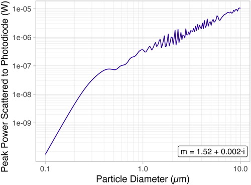
The model predicts that larger particles have a higher probability of generating enough scattered light power to the photodiode to be detected. For example, a 10-µm particle that passes through the focal point of the laser generates a peak power at the photodiode of 1.11⋅10⁻⁵ W; however, 10-µm particles that miss the focal point and generate only 0.35% of this peak power are still detected at the 3.13⋅10⁻⁸ W limit and are counted. Particles smaller than 0.5 µm need to intersect the focal point or very close to it to generate enough power at the photodiode to be detected. The effective sensing volume for 0.5-μm particles is a cylinder with a length of 0.6 mm and a diameter of 0.04 mm (Figure S47). The sensing volume is larger for larger diameter particles. The model predicts that approximately 0.03% of 0.40-µm particles and 2.4% of 10-µm particles are detected and counted (Figure S48).

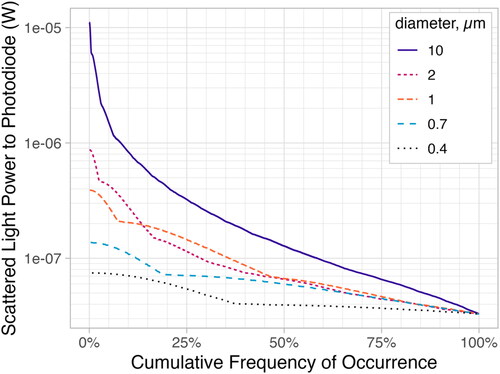
Although large particles have a higher probability of being detected by the PMS5003 than small particles, most of them generate power to the photodiode corresponding to a smaller diameter because they miss the laser focal point. The PMS5003 microprocessor is unable to differentiate pulses of the same amplitude, whether they are from a 0.4-µm particle passing through the focal point or from a 4-µm particle missing the focal point. The model-predicted frequency of scattered light power for various particle diameters is shown in Figure 4.

Figure 4. Model-predicted cumulative frequency of scattered light power for different particle diameters assuming a refractive index of 1.52 + i0.002.

The fraction of particles of various sizes that the model predicts would be sized correctly, depending on the fraction of peak power that a particle must generate to be assigned the correct size, is shown in Table 1 for particles having a 1.52 + i0.002 refractive index. If the PMS5003 were a perfect OPC, these fractions would be 1.0 for all sizes. If the PMS5003 uses a cutoff criterion of 50% of peak power, then 72.4% of 0.40-µm particles would be sized correctly, but only 13.4% of 1.0-µm particles would be sized correctly. The remainder of the 1.0-µm particles, 86.6%, would be sized smaller than 1.0 µm. The 10-µm particles would be almost invisible to the PMS5003 because 99% of them would be sized smaller than 10 µm.

Table 1. Model-predicted fraction of particles being sized correctly, as a function of percent of peak power.

Dp, µm	Peak power at photodiode, W	Probability of particle exceeding % of peak power
		30% of peak	50% of peak	70% of peak	90% of peak
0.4	7.46⋅10^−8	1.000	0.724	0.262	0.131
0.7	1.37⋅10^−7	0.818	0.340	0.128	0.067
1.0	3.89⋅10^−7	0.314	0.135	0.052	0.027
2.0	8.73⋅10^−7	0.107	0.047	0.018	0.009
10.0	1.11⋅10^−5	0.021	0.010	0.003	0.002

If a particle generates a power equal to or greater than a fraction of its peak power, then it is assumed to be “correctly” sized by the PMS5003.

The model-predicted particle sizing efficiency PSE(D_p) in Table 1 can be approximated as a damped exponential: (16) $$\mathrm{PSE}\left(D_p\right)=\exp \left[-3.22\log \hspace{0.17em}\left(D_p/0.30\mathrm{ }\mu m\right)\right]$$(16)

As shown in Table 2, most particles smaller than 2 µm would be assigned to the 0.3–0.5 µm PMS5003. Because the model predicts that the PMS5003 undercounts the actual particle number concentrations for a given diameter, any calculations that use the particle number distribution, such as the scattering coefficient or the mass concentration, would be affected. If the PMS5003 uses a 50% peak power criterion, the model predicts that the PMS5003 scattering coefficients for 0.40- and 1.0-µm particles would be 72.4% and 13.5% of the true values, respectively. The model predicts that the PMS5003 would severely underestimate the mass concentration between 2.5 µm and 10 µm (i.e., PM₁₀ – PM_2.5), estimating only 2% to 10% of the true value.

Table 2. Model-predicted apportionment of particles of various diameters to PMS5003 particle size bins.

Dp, µm	PMS5003 apportionment to particle size bin
	0.3–0.5 µm	0.5–1.0 µm	1.0–2.5 µm	2.5–5.0 µm	5.0–10.0 µm
0.2	0.00	0.00	0.00	0.00	0.00
0.3	1.00	0.00	0.00	0.00	0.00
0.5	1.00	0.00	0.00	0.00	0.00
0.7	0.83	0.17	0.00	0.00	0.00
1.0	0.55	0.45	0.00	0.00	0.00
2.0	0.61	0.32	0.06	0.00	0.00
10.0	0.32	0.47	0.12	0.07	0.02

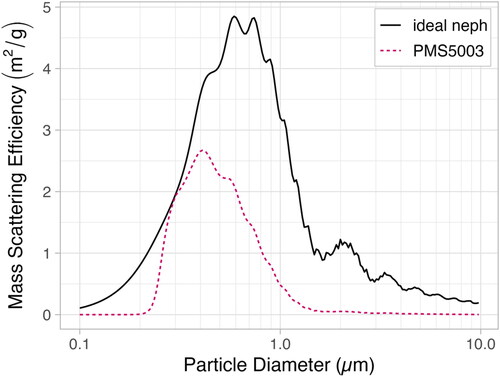
3.6. PMS5003 mass scattering efficiency

The predicted mass scattering efficiency for the PMS5003 measuring dry ammonium sulfate aerosol (calculated using Equations (15)(15) $$b_{sp}=0.015CH1$$(15) and (16)(16) $$\mathrm{PSE}\left(D_p\right)=\exp \left[-3.22\log \hspace{0.17em}\left(D_p/0.30\mathrm{ }\mu m\right)\right]$$(16) ) is compared to the theoretical mass scattering efficiency (calculated using Equation (14)(14) $$E_{ms}^{\prime }\left(D_p,\rho ,m,\mathrm{\lambda }\right)=\frac{b_{sp}^{\prime }}{M}=\frac{\mathrm{PSE}\left(D_p\right)·b_{sp}}{M}=\mathrm{PSE}\left(D_p\right)·E_{ms}\left(D_p,\rho ,m,\mathrm{\lambda }\right)$$(14) ) in Figure 5. The differences between the PMS5003 mass scattering efficiency and the theoretical mass scattering efficiency are relatively small for 0.3-µm to 0.4-µm particles but are substantial for larger diameter particles. For example, if PMS5003-reported PM_2.5 concentrations are calibrated against a regulatory PM_2.5 monitor using an aerosol with a mass median diameter of 0.6 µm, then Equations (15)(15) $$b_{sp}=0.015CH1$$(15) and (16)(16) $$\mathrm{PSE}\left(D_p\right)=\exp \left[-3.22\log \hspace{0.17em}\left(D_p/0.30\mathrm{ }\mu m\right)\right]$$(16) predict that the PSM5003 would overestimate regulatory PM_2.5 concentrations by a factor of 2 for an aerosol with a mass median diameter of 0.4 µm.

Figure 5. Mass scattering efficiency (MSE) for dry ammonium sulfate aerosol (density = 1.7 g cm⁻³; refractive index at 657 nm = 1.51 + 0i). The theoretical MSE is shown by the solid line. The truncated PMS5003 MSE, shown by the dashed line, is calculated from Equation (14)(14) $$E_{ms}^{\prime }\left(D_p,\rho ,m,\mathrm{\lambda }\right)=\frac{b_{sp}^{\prime }}{M}=\frac{\mathrm{PSE}\left(D_p\right)·b_{sp}}{M}=\mathrm{PSE}\left(D_p\right)·E_{ms}\left(D_p,\rho ,m,\mathrm{\lambda }\right)$$(14) with T(D_p) from Figure 4.

Additionally, although Plantower claims the PMS5003 has a 50% efficiency detection limit of 0.3 µm, the aerosol used to measure this detection limit is not reported. If the PMS5003 is calibrated at Plantower headquarters in Beijing with an ambient aerosol having a refractive index of 1.48 + i0.011 (Che et al. 2008; Li et al. 2013), our model predicts that U.S. background aerosol and smoke would be detected at smaller diameters and would generate more power to the photodiode than the Beijing aerosol (Figure S57). The resultant number and mass concentrations reported by the PMS5003 for U.S. ambient aerosol would then be higher than for the Beijing calibration aerosol. Thus, our model demonstrates how a difference between the refractive index of the aerosol used to calibrate the PMS5003 and the refractive index of typical U.S. ambient aerosol would contribute to PMS5003-reported PM_2.5 exceeding regulatory values (see SI Section S3.5.6 for additional details). Overall, our modeling results help explain why prior studies have reported that the PMS5003 often overreports ambient PM_2.5 and wildfire smoke concentrations in the U.S. (Barkjohn, Gantt, and Clements 2021; Delp and Singer 2020; Holder et al. 2020).

3.7. Evaluating the PMS5003 physical-optical model against laboratory data

3.7.1. PSL size bins

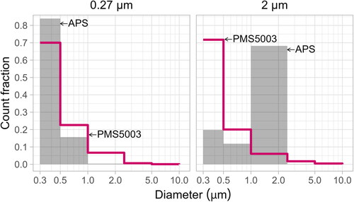
The PMS5003 did not assign the 2.0-µm PSL spheres measured by Tryner et al. (2020a) to the correct 1.0 to 2.5 µm size bin; instead, it assigned over 90% of them to the submicron size bins (Figure 6). This experimental result is consistent with our model predictions in Table 2 and the findings of He, Kuerbanjiang, and Dhaniyala (2020). Our model predicts that approximately 93% of 2.0-µm particles with 1.52 + i0.002 refractive index will be assigned a particle size less than 1 µm by the PMS5003.

Figure 6. PMS5003- and APS3321-reported number concentration distributions for 0.27 and 2.0 µm PSL spheres (m = 1.59 + 0.0i). The relative count fractions for the PMS5003 are nearly constant for the two aerosols, despite the differences captured by the APS.

3.7.2. Scattering coefficient reduction

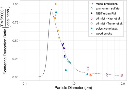
Our physical-optical model predicts that the PMS5003 scattering coefficient would be reduced relative to the true scattering coefficient as particle diameter increases due to the reduced fraction of correctly-sized particles. Model predictions of scattering coefficient reduction with particle diameter are consistent with the laboratory results for a variety of aerosol types with scattering coefficient median diameters ranging from 0.40 to 10 µm (Figure 6). This agreement suggests that the reason for the PMS5003’s poor performance for coarse particles is primarily due to its counting and sizing inefficiency, not poor aspiration efficiency (Figure 7).

Figure 7. PMS5003 scattering coefficient truncation vs. scattering coefficient median diameter. The dashed line is a fit of the model-predicted fraction of particles that are sized correctly (50% of peak power) from Table 1. The solid line assumes the Plantower-reported 50% counting efficiency at 0.30 µm and 1% counting efficiency at 0.20 µm. The points are scattering coefficient ratios that were calculated from aerosol size distribution data collected by Tryner et al. (2020b) and Kaur and Kelly (2023b) using the relationship between scattering efficiency and PMS5003-reported count of particle > 0.3 µm reported by Ouimette et al. (2022).

3.7.3. PMS5003 response to relative humidity (RH)

As RH increased, the “reference” wet PM_2.5 concentration calculated from SMPS and APS data increased exponentially, relative to the dry PM_2.5 concentration, consistent with classic hygroscopic behavior. The PMS5003-reported wet PM_2.5 concentration also increased, but less than the reference wet PM_2.5 concentration and approximately linearly. The PMS5003-reported wet PM_2.5 was 45% less than the reference wet PM_2.5 at 89% RH.

As RH increased from 21% to 89%, the ammonium sulfate mass median diameter (MMD) increased from 0.79 to 1.18 µm, its density dropped from 1.70 to 1.24 g cm⁻³, and its refractive index dropped from 1.51 to 1.36. Theoretical mass scattering efficiencies for these aerosols are 4.42 m² g⁻¹ (for MMD = 0.78 µm) and 4.46 m² g⁻¹ (for MMD = 1.18 µm); in other words, the ammonium sulfate theoretical mass scattering efficiency remained approximately unchanged as the RH increased from 21% to 89%. In contrast, the ammonium sulfate mass scattering efficiency inside the PMS5003 decreased by 60%, from 1.10 m² g⁻¹ at 0.79 µm to 0.45 m² g⁻¹ at 1.18 µm, as the RH increased from 21% to 89% (see Figure S54). This decrease occurred because the aerosol grew into a diameter for which the PMS5003 was less effective in counting and sizing (see Table 1 and Figure 4). Thus, the model predicts that the PMS5003 would underestimate the wet PM_2.5 at 89% RH by approximately 60%. This prediction is consistent with the laboratory data, which indicated that the PMS5003 underestimated the reference wet PM_2.5 concentration by approximately 45% at RH = 89% (Figure S52). The agreement is within the uncertainty in measurement.

3.8. Modeling PurpleAir/PMS5003 sampling efficiency with computational fluid dynamics

The PurpleAir CFD model results show that as flow moves around the enclosure, at the bottom, flow accelerates and moves away from the opening. Depending on wind speed, coarse particles are not able to follow the streamlines. A recirculation region with low speed is observed in the vicinity of the PMS5003 sensors. This recirculation region is the primary source of ambient air at the sensor sampling location within the PA enclosure.

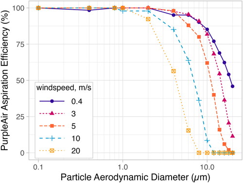
The sampling efficiency of particles entering the PA enclosure obtained from the CFD simulations is shown in Figure 8. For particles smaller than 1 µm, the sampling efficiency was 100% for all wind speeds studied (i.e., 0.4 to 20 m s⁻¹). For larger particles, the sampling efficiency decreased with wind-speed. The 50% sampling efficiency cut size of particles entering the PA enclosure was ∼15 µm for 0.4 m s⁻¹, reducing to ∼2.5 µm for 20 m s⁻¹. For low-wind speeds (less than 3 m s⁻¹), particles over the entire size range of PMS5003 detection (i.e., up to 10 µm) were available within the PA enclosure. The PMS5003 flow rate had no significant effect on the modeled results. While the availability of particles in the PA enclosure doesn’t necessarily result in their sampling and transmission to the detection region of the PMS5003, the non-availability of particles in the PA enclosure at higher wind-speeds implies that these particles would be under-represented in the PA signal relative to actual ambient values. Additional results from the CFD model can be found in SI Section 3.6.

Figure 8. Sampling efficiency of particles as a function of aerodynamic diameter and ambient wind-speed.

When the PMS5003 sensor that had operated in Austin, Nevada, USA for two years was disassembled, it was evident that coarse aerosol from windblown dust was able to enter the sensor, consistent with the CFD aspiration model predictions in Figure 8. Because of the orientation of the PMS5003 sensors in the PurpleAir with respect to gravity, both impaction and sedimentation losses before and after detection were observed (see photographs in Figures S62–S64). No quantitative measurements were made of the transmission losses, and it is not known if our results are representative of other PurpleAir monitors that sample significant windblown dust. We conclude that the PMS5003’s poor performance for coarse particles is primarily due to its counting inefficiency, not poor aspiration efficiency.

4. Summary and conclusions

Users of the Plantower PMS5003 sensor have long debated whether it operates as a reciprocal nephelometer (Ouimette et al. 2022) or an optical particle counter. If the PMS5003 operated as a reciprocal nephelometer, it would have the following characteristics:

• It would measure the light scattering from an ensemble of particles which all experience the same intensity of light from a collimated beam. A typical reciprocal nephelometer uses, for example, an opal glass diffuser before the detector to properly weigh the light scattered by all the particles along the light beam.

• The output from the PMS5003 photodetector would usually be a slowly varying signal from the cloud of particles, and not consist of a series of short duration discrete pulses.

• Modest changes in the sample flow rate would not affect the reported number concentration because the active scattering volume contains many particles with relatively long residence times in the scattering volume, typically 0.1 to 0.3 s.

• The PMS5003 would detect nephelometer calibration gases such as Suva^TM and CO₂.

Our results demonstrate that none of these characteristics are true.

• The PMS5003 has a focused Gaussian laser beam. Particles do not experience the same intensity of light as they flow through various regions of the beam.

• The output from the photodiode consists of discrete pulses. These pulses have widths of 20–800 µs, consistent with the width of the focused laser, the flow rate through the sensing volume, and passage of individual particles. Pulse amplitudes are correlated with the particle size concentration bins.

• Small flow rate reductions result in proportional reductions in the reported total number concentration because the PMS5003 counts pulses like an OPC.

• The PMS5003 does not detect Suva^TM or CO₂ calibration gases (Ouimette et al. 2022) because the PMS5003 uses a high pass filter to remove slowly varying and DC voltage components.

In summary, the PMS5003 does not operate as a reciprocal nephelometer, but does have one characteristic that makes it a good surrogate nephelometer: the value of the PMS5003 total number concentration (“CH1”) is strongly correlated with the submicron aerosol scattering coefficient over four orders of magnitude (Ouimette et al. 2022).

The PMS5003 does function as an imperfect optical particle counter that can detect and count particles as small as 0.3 µm diameter; however, it has serious limitations as an OPC. Typically, all particles that flow through an OPC are irradiated with the same intensity of light. Like an OPC, the PMS5003 detects particles individually; however, it is unable to size them correctly because detected particles of different diameters may produce the same photodiode power, depending on where they intersect the laser beam. Our physical-optical model results demonstrate that the sensor has poor sizing efficiency for particles larger than 1 µm. More than 99% of the particles miss the PMS5003 laser, and those that intercept the laser usually miss the focal point and are undersized by the photodiode-microprocessor combination.

Additionally, our experimental modeling results demonstrate that the flow rate through the PMS5003 sensor and, consequently, sensor-reported PM data are highly sensitive to 1 Pa to 2.5 Pa flow impedances at the inlet. Our CFD modeling results demonstrate that, for PMS5003 sensors installed in PurpleAir housings, the sampling efficiency of l µm to 10 µm particles will decrease at wind speeds greater than 3 m s⁻¹, potentially affecting the data reported by the sensors. Designers of monitors that integrate the PMS5003 into a secondary housing and users of such monitors should keep these limitations in mind.

Disclosure statement

No potential conflict of interest was reported by the authors.

Additional information

Funding

This work was supported by grants from the National Institute for Occupational Safety and Health (OH011660) and National Institute of Environmental Health Sciences (ES024041).

References

- Agarwal, J. K., and B. Y. H. Liu. 1980. A criterion for accurate aerosol sampling in calm air. Am. Ind. Hyg. Assoc. J. 41 (3):191–7. doi: 10.1080/15298668091424591.
- Barkjohn, K. K., B. Gantt, and A. L. Clements. 2021. Development and application of a United States-wide correction for PM2.5 data collected with the PurpleAir sensor. Atmos. Meas. Tech. 4 (6):4617–37. doi: 10.5194/amt-14-4617-2021.
- Belyaev, S. P., and L. M. Levin. 1974. Techniques for collection of representative aerosol samples. J. Aerosol Sci. 5 (4):325–38. doi: 10.1016/0021-8502(74)90130-X.
- Bittner, A. S., E. S. Cross, D. H. Hagan, C. Malings, E. Lipsky, and A. P. Grieshop. 2022. Performance characterization of low-cost air quality sensors for off-grid deployment in rural Malawi. Atmos. Meas. Tech. 15 (11):3353–76. doi: 10.5194/amt-15-3353-2022.
- Che, H., G. Shi, A. Uchiyama, A. Yamazaki, H. Chen, P. Goloub, and X. Zhang. 2008. Intercomparison between aerosol optical properties by a PREDE skyradiometer and CIMEL sunphotometer over Beijing, China. Atmos. Chem. Phys. 8 (12):3199–214. doi: 10.5194/acp-8-3199-2008.
- Cheeseman, M. J., B. Ford, S. C. Anenberg, M. J. Cooper, E. V. Fischer, M. S. Hammer, S. Magzamen, R. V. Martin, A. Van Donkelaar, J. Volckens, et al. 2022. Disparities in air pollutants across racial, ethnic, and poverty groups at US public schools. Geohealth 6 (12):e2022GH000672. doi: 10.1029/2022GH000672.
- Chen, L., X. Pang, J. Li, B. Xing, T. An, K. Yuan, S. Dai, Z. Wu, S. Wang, Q. Wang, et al. 2022. Vertical profiles of O3, NO2 and PM in a major fine chemical industry park in the Yangtze River Delta of China detected by a sensor package on an unmanned aerial vehicle. Sci. Total Environ. 845:157113. doi: 10.1016/j.scitotenv.2022.157113.
- Davies, C. N. (1968). The entry of aerosols into sampling tubes and heads. J. Phys. D: Appl. Phys. 1 (7):921–932. doi: 10.1088/0022-3727/1/7/314.
- Delp, W. W., and B. C. Singer. 2020. Wildfire smoke adjustment factors for low-cost and professional PM2.5 monitors with optical sensors. Sensors (Basel) 20 (13):3683. doi: 10.3390/s20133683.
- Dhammapala, R., A. Basnayake, S. Premasiri, L. Chathuranga, and K. Mera. 2022. PM2.5 in Sri Lanka: Trend analysis, low-cost sensor correlations and spatial distribution. Aerosol Air Qual. Res. 22 (5):210266. doi: 10.4209/aaqr.210266.
- Do, K., H. Yu, J. Velasquez, M. Grell-Brisk, H. Smith, and C. E. Ivey. 2021. A data-driven approach for characterizing community scale air pollution exposure disparities in inland Southern California. J. Aerosol Sci. 152:105704. doi: 10.1016/j.jaerosci.2020.105704.
- Dubey, R., A. K. Patra, and Nazneen. (2022). Vertical profile of particulate matter: A review of techniques and methods. Air Qual. Atmos. Health 15 (6):979–1010. doi: 10.1007/s11869-022-01192-1.
- Fanti, G., F. Borghi, A. Spinazzè, S. Rovelli, D. Campagnolo, M. Keller, A. Cattaneo, E. Cauda, and D. M. Cavallo. 2021. Features and practicability of the next-generation sensors and monitors for exposure assessment to airborne pollutants: A systematic review. Sensors (Basel) 21 (13):4513. doi: 10.3390/s21134513.
- Fire and Smoke Map. 2023. AirNow. Accessed August 15, 2023. https://fire.airnow.gov.
- Glib, J., A. Mortier, M. Schulz, E. Andrews, Y. Balkanski, S. E. Bauer, A. M. K. Benedictow, H. Bian, R. Checa-Garcia, M. Chin, et al. 2021. AeroCom phase III multi-model evaluation of the aerosol life cycle and optical properties using ground- and space-based remote sensing as well as surface in situ observations. Atmos. Chem. Phys. 21 (1):87–128. doi: 10.5194/acp-21-87-2021.
- Goodfellow, H. D. and R. Kosonen, eds. 2020. Industrial ventilation design guidebook. Vol. 1. Waltham, MA: Academic Press.
- Hagan, D. H., and J. H. Kroll. 2020. Assessing the accuracy of low-cost optical particle sensors using a physics-based approach. Atmos. Meas. Tech. 13 (11):6343–55. doi: 10.5194/amt-13-6343-2020.
- Hangal, S., and K. Willeke. 1990. Aspiration efficiency: Unified model for all forward sampling angles. Environ. Sci. Technol. 24 (5):688–91. doi: 10.1021/es00075a012.
- He, M., N. Kuerbanjiang, and S. Dhaniyala. 2020. Performance characteristics of the low-cost Plantower PMS optical sensor. Aerosol Sci. Technol. 54 (2):232–41. doi: 10.1080/02786826.2019.1696015.
- Hofman, J., M. Nikolaou, S. P. Shantharam, C. Stroobants, S. Weijs, and V. P. La Manna. 2022. Distant calibration of low-cost PM and NO2 sensors; evidence from multiple sensor testbeds. Atmos. Pollut. Res. 13 (1):101246. doi: 10.1016/j.apr.2021.101246.
- Holder, A. L., A. K. Mebust, L. A. Maghran, M. R. McGown, K. E. Stewart, D. M. Vallano, R. A. Elleman, and K. R. Baker. 2020. Field evaluation of low-cost particulate matter sensors for measuring wildfire smoke. Sensors (Basel) 20 (17):4796. doi: 10.3390/s20174796.
- Jaffe, D. A., C. Miller, K. Thompson, B. Finley, M. Nelson, J. Ouimette, and E. Andrews. 2023. An evaluation of the U.S. EPA’s correction equation for PurpleAir sensor data in smoke, dust, and wintertime urban pollution events. Atmos. Meas. Tech. 16 (5):1311–22. doi: 10.5194/amt-16-1311-2023.
- Jain, S., A. A. Presto, and N. Zimmerman. 2021. Spatial modeling of daily PM2.5, NO2, and CO concentrations measured by a low-cost sensor network: comparison of linear, machine learning, and hybrid land use models. Environ. Sci. Technol. 55 (13):8631–41. doi: 10.1021/acs.est.1c02653.
- Kaur, K., and K. E. Kelly. 2023a. Performance evaluation of the Alphasense OPC-N3 and Plantower PMS5003 sensor in measuring dust events in the Salt Lake Valley, Utah. Atmos. Meas. Tech. 16 (10):2455–70. doi: 10.5194/amt-16-2455-2023.
- Kaur, K., and K. E. Kelly. 2023b. Laboratory evaluation of the Alphasense OPC-N3, and the Plantower PMS5003 and PMS6003 sensors. J. Aerosol Sci. 171:106181. doi: 10.1016/j.jaerosci.2023.106181.
- Lee, C.-H., Y.-B. Wang, and H.-L. Yu. 2019. An efficient spatiotemporal data calibration approach for the low-cost PM2.5 sensing network: A case study in Taiwan. Environ. Int. 130:104838. doi: 10.1016/j.envint.2019.05.032.
- Levy Zamora, M., C. Buehler, A. Datta, D. R. Gentner, and K. Koehler. 2023. Identifying optimal co-location calibration periods for low-cost sensors. Atmos. Meas. Tech. 16 (1):169–79. doi: 10.5194/amt-16-169-2023.
- Li, Z., X. Gu, L. Wang, D. Li, Y. Xie, K. Li, O. Dubovik, G. Schuster, P. Goloub, Y. Zhang, et al. 2013. Aerosol physical and chemical properties retrieved from ground-based remote sensing measurements during heavy haze days in Beijing winter. Atmos. Chem. Phys. 13 (20):10171–83. doi: 10.5194/acp-13-10171-2013.
- Malings, C., R. Tanzer, A. Hauryliuk, P. K. Saha, A. L. Robinson, A. A. Presto, and R. Subramanian. 2020. Fine particle mass monitoring with low-cost sensors: Corrections and long-term performance evaluation. Aerosol Sci. Technol. 54 (2):160–74. doi: 10.1080/02786826.2019.1623863.
- Mei, H., P. Han, Y. Wang, N. Zeng, D. Liu, Q. Cai, Z. Deng, Y. Wang, Y. Pan, and X. Tang. 2020. Field evaluation of low-cost particulate matter sensors in Beijing. Sensors (Basel) 20 (16):4381. doi: 10.3390/s20164381.
- Molina Rueda, E., E. Carter, C. L'Orange, C. Quinn, and J. Volckens. 2023. Size-resolved field performance of low-cost particulate matter sensors. Environ. Sci. Technol. Lett. 10 (3):247–53. doi: 10.1021/acs.estlett.3c00030.
- Moosmuller, H., and C.-Y. She. 1991. Equal intensity and phase contours in focused Gaussian laser beams. IEEE J. Quantum Electron. 27 (4):869–74. doi: 10.1109/3.83316.
- Nguyen, P. D. M., N. Martinussen, G. Mallach, G. Ebrahimi, K. Jones, N. Zimmerman, and S. B. Henderson. 2021. Using low-cost sensors to assess fine particulate matter infiltration (PM2.5) during a wildfire smoke episode at a large inpatient healthcare facility. Int. J. Environ. Res. Public Health 18 (18):9811. doi: 10.3390/ijerph18189811.
- Ouimette, J. R., W. C. Malm, B. A. Schichtel, P. J. Sheridan, E. Andrews, J. A. Ogren, and W. P. Arnott. 2022. Evaluating the PurpleAir monitor as an aerosol light scattering instrument. Atmos. Meas. Tech. 15 (3):655–76. doi: 10.5194/amt-15-655-2022.
- Pang, X., L. Chen, K. Shi, F. Wu, J. Chen, S. Fang, J. Wang, and M. Xu. 2021. A lightweight low-cost and multipollutant sensor package for aerial observations of air pollutants in atmospheric boundary layer. Sci. Total Environ. 764:142828. doi: 10.1016/j.scitotenv.2020.142828.
- Petters, M. D., and S. M. Kreidenweis. 2007. A single parameter representation of hygroscopic growth and cloud condensation nucleus activity. Atmos. Chem. Phys. 7 (8):1961–71. doi: 10.5194/acp-7-1961-2007.
- Pharis, N., J. Habeck, J. Douglas, J. Meiners, A. Ally, P. Collins, and J. Flaten. 2022. Modifying and calibrating low-cost optical particle counters for stratospheric ballooning use. In 2020 Academic High Altitude Conference, Presented at the 2020 Academic High Altitude Conference, Iowa State University Digital Press. doi: 10.31274/ahac.11650.
- Snider, G., C. L. Weagle, R. V. Martin, A. Van Donkelaar, K. Conrad, D. Cunningham, C. Gordon, M. Zwicker, C. Akoshile, P. Artaxo, et al. 2015. SPARTAN: A global network to evaluate and enhance satellite-based estimates of ground-level particulate matter for global health applications. Atmos. Meas. Tech. 8 (1):505–21. doi: 10.5194/amt-8-505-2015.
- Solomon, P. A., andS. Dhaniyala. 2020. Preface. Aerosol Sci. Technol. 54 (2):143–6. doi: 10.1080/02786826.2020.1706973.
- Sun, Y., A. Mousavi, S. Masri, and J. Wu. 2022. Socioeconomic disparities of low-cost air quality sensors in California, 2017–2020. Am. J. Public Health. 112 (3):434–42. doi: 10.2105/AJPH.2021.306603.
- Tengono, J. 2022. Personal Communication with Jim Ouimette.
- Tryner, J., J. Mehaffy, D. Miller-Lionberg, and J. Volckens. 2020a. Effects of aerosol type and simulated aging on performance of low-cost PM sensors. J. Aerosol Sci. 150:105654. doi: 10.1016/j.jaerosci.2020.105654.
- Tryner, J., J. Mehaffy, D. Miller-Lionberg, and J. Volckens. 2020b. Dataset associated with “Effects of aerosol type and simulated aging on performance of low-cost PM sensors. https://hdl.handle.net/10217/207239.
- Zieger, P., R. Fierz-Schmidhauser, E. Weingartner, and U. Baltensperger. 2013. Effects of relative humidity on aerosol light scattering: Results from different European sites. Atmos. Chem. Phys. 13 (21):10609–31. doi: 10.5194/acp-13-10609-2013.