Dose distributions in SBRT of lung tumors: Comparison between two different treatment planning algorithms and Monte-Carlo simulation including breathing motions

Abstract

In stereotactic body radiotherapy (SBRT) of lung tumors, dosimetric problems arise from: 1) the limited accuracy in the dose calculation algorithms in treatment planning systems, and 2) the motions with the respiration of the tumor during treatment.

Longitudinal dose distributions have been calculated with Monte Carlo simulation (MC), a pencil beam algorithm (PB) and a collapsed cone algorithm (CC) for two spherical lung tumors (2 cm and 5 cm diameter) in lung tissue, in a phantom situation. Respiratory motions were included by a convolution method, which was validated. In the static situation, the PB significantly overestimates the dose, relative to MC, while the CC gives a relatively accurate estimate. Four different respiratory motion patterns were included in the dose calculation with the MC. A “narrowing” of the longitudinal dose profile of up to 20 mm (at about 90% dose level) is seen relative the static dose profile calculated with the PB.

Local relapse after radical radiotherapy of solid tumors is a significant problem in several anatomical sites, using conventional doses and fractionation schedules. Insufficient dose to the target is expected to be the major cause. The dose and volume of the dose restricting normal tissues can be minimized by improved geometrical accuracy and reproducibility in the dose delivery. One way to obtain this for intracranial targets has been stereotactic radiotherapy/radiosurgery, which has been used for many decades.

For extracranial targets, a method for stereotactic radiotherapy (today the acronym SBRT–stereotactic body radiotherapy, is widely used and will be used here) was developed in the early 1990's at the Karolinska hospital, which has been previously described [1], [2]. The main aspects of the method are: 1) the use of a stereotactic body frame for stereotactic CT/MR localization of the target as well as stereotactic set-up at the treatment unit; 2) Direct, tomographic verification-imaging (CT) of the position of the target in the stereotactic reference system. The points 1) and 2) make it possible to reduce the margin between clinical target volume (CTV) and planning target volume (PTV); 3) A planned very heterogeneous dose distribution within the PTV, which makes possible a considerable increase of the dose to the CTV compared to the conventional approach with a homogeneous dose distribution within the PTV. The higher dose to the CTV is obtained for an essentially invariant dose outside PTV; as a consequence the cell kill within the tumor will increase for a given toxicity level [1], [3]; 4) A very high target dose is delivered in a short time, which gives a high biological effect in the tumor. Typically 15–20 Gy×3 is delivered to the CTV during one week, corresponding to 95–150 Gy in 2 Gy fractions.

The SBRT method was introduced into clinical practice in 1991 at Karolinska Hospital, and has today been spread to many other centers [4]. Its main clinical application today is the treatment of primary and metastatic lung tumors, and the second most common location is the treatment of tumors in the liver. Both of these tumor locations are affected by the respiratory motion in the body, which primarily is a longitudinal (cranial-caudal) motion. In the SBRT method, abdominal compression is used for targets which are affected by large breathing motions, whereby the longitudinal motion almost always can be reduced to within 10 mm [2]. Despite this reduction of motion, the dose distribution calculated in the static situation is different from the one that is delivered in the patient. This paper deals with the impact on the dose distribution from the respiration motion.

The above problem was mathematically corrected for by a convolution of the dose distribution calculated for the static situation with a probability distribution function (pdf) which describes the nature of the motion, by Lujan [5]. This method was developed for situations in which the dose distribution is invariant for small changes in the target position. This is relevant for unit density tissues, as an example the treatment of a tumor in the liver. For tumors in the lungs, a method for fluence convolution, instead of dose convolution, to take the lack of dose invariance into account, has been described in references [6], [7].

In the literature, several functions have been assumed to describe different forms of breathing motions; for example a linear motion (saw tooth), a harmonic oscillator and cos²ⁿ. The most complete description of the motion pattern, including occasional deep breaths, changes in the breathing frequency, and changes by time of the relative lengths of the inhale and exhale phases was given by George et al. [8]. They presented the pdf of the entire respiratory motion, based on data from measurements on patients.

For SBRT of tumors in the lungs there is a well known problem of the accuracy of the dose calculation in commercial treatment planning systems, in which secondary particles are dealt with in a more or less approximate manner. Especially underestimation of the range of Compton electrons in lung tissue in pencil-beam (PB) models leads to dose errors, primarily close to the interface between the solid tumor and the lung tissue. Improved dose calculation models are implemented in some systems, such as collapsed-cone (CC) algorithms, in which the range of Compton electrons are better taken into account. However, Monte-Carlo simulation, based on first principles of physics, is the most accurate dose calculation method in treatment planning available today.

In this paper the Monte-Carlo code PENELOPE was used to calculate the longitudinal dose distribution in two phantom cases with spherical, unit density tumors, positioned in lung tissue. To incorporate the effect of the breathing motion on the dose distribution, published data on four different pdf's were used. As a comparison, static dose distributions were also calculated with a PB model and a CC model.

Material and methods

Dose calculations in the static situation

Dose calculations were made for two phantom cases. One for a 2 cm and the other one for a 5 cm diameter spherical tumor, located centrally in lung tissue. The density of the lung tissue was defined as 0.30 g/cm³ and the tumors were water equivalent with unit density. The choice of lung density was made according to ICRP specifications following PENELOPE material files. Figure 1a shows the geometry for the two cases, and the pentagonal phantom. The lung and “chest wall” was 2D, i.e. with the same cross section in the longitudinal extent of the phantom.

Figure 1.  Cross section of the pentagonal phantom. The entrances of the five beams are indicated. The two spherical, water equivalent GTVs are for illustration purposes drawn on top of each other. The longitudinal axis of the phantom is z. b. Outline of the blocked beams for the two cases. CTV was defined to be the same as GTV (diameters of 2 cm and 5 cm). The margin to the PTV was 1.0 cm in all directions.

In clinical practice five beams is a reasonable number in SBRT of relatively symmetrically shaped lung tumors. For these cases it was also assumed, from clinical practice, that the margin between GTV (here equal to CTV) and PTV was 10 mm in all directions. This margin is used at the Karolinska for lung tumors that are not fixed to the pleura or mediastinal structures. In case the tumor is fixed, the transverse margin reduces to 5 mm, and the longitudinal 10 mm.

Dose planning was made with a PB model (TMS system v 6.1b) that is used in our clinical practice, with 5 beams of 6 MV from a Varian 2300 CD accelerator. Isocenter was positioned in the centre of GTV (Figure 1a). In SBRT, the multi-leaf collimator (MLC) of the accelerator is used for obtaining irregularly shaped beams. However, in this case, blocks were defined in order to simplify the beam geometry and also to get a dose distribution more conformal to the PTV. The shape of the blocks used in the beams, were determined so as to have the prescribed 100% isodose circumscribing the PTV as close as possible (but not necessarily exactly (cf Figure 3)) and with a dose to the centre of the tumor equal to 150%, according to clinical practice at Karolinska. The blocks were positioned at the distance of the shadow tray of the Varian accelerator. Figure 1b shows the outline of the blocked beams for the two cases. The jaws of the accelerator were set to 10 cm×10 cm. With the beams determined in this way, the dose distribution was calculated along the longitudinal (z) axis, through the centre of the tumor for each case. Similar calculations were also made with a collapsed-cone (CC) model (Pinnacle system v 6.2b) for the same beams, with the same output (number of monitor units (MU)) for the two calculation models.

Monte Carlo (MC) simulations in the same geometry configurations as described above were conducted with the PENELOPE code system [9] combined with PENEASY [10], a generic main program and accessory routines that allow an easy configuration of PENELOPE. PENELOPE performs Monte Carlo simulation of coupled electron-photon transport in arbitrarily defined materials in the energy range from 50 eV up to 1 GeV. Photon transport is simulated by means of the detailed simulation scheme, i.e., interaction by interaction. Electron and positron histories are generated on the basis of a mixed procedure, which combines detailed simulation of hard events (those involving energy losses or angular deflections above certain user-defined cut offs, here WCR = 500 keV and WCC = 10 keV were used) with condensed simulation of soft interactions which make this code very efficient in the particular case of interfaces between materials of different densities [11].

To reduce the calculation time, the simulation was divided in two parts. First the Phase Space Files (PSFs) of the 6MV photon beams were generated by simulating the Varian accelerator head following the manufacturer specifications, both for open beams and for the blocked beams described above. The total number of particles stored in the PSFs was of the order of 10⁵ particles per cm², which allowed obtaining good statistical uncertainties in any dose calculations. The PSFs were validated by comparing the measured and calculated percentage depth doses and lateral profiles in a water phantom, placed in standard reference conditions, according to the TG53 [12].

These calculated beams were then used as sources to obtain longitudinal dose profiles and depth doses in the phantom cases with a voxel resolution between 1 and 8 mm³ (with statistical uncertainties within 1.5% for 1 s.d.). Due to the small dimensions of the voxels, in order to improve statistics, a splitting variance reduction technique was applied to re-use the generated PSF.

In order to be able to compare MC, PB, CC data the same number of monitor units (MU) was used in all three computation methods. For this purpose, absolute dose calibration was performed in the MC system to covert MC-doses into absolute doses.

Following a previous work [13], the calibration set-up was created by first simulating, for each different field, the absorbed dose in a small cylinder (with dimensions similar to a ionisation chamber) placed in a water phantom in reference conditions (at Karolinska; SSD = 95 cm and 5 cm phantom depth). To this MC-dose value a predetermined output MU/Gy was assigned (Table I) to determine a conversion factor. This conversion factor was then used to determine the dose given in each voxel in the lung phantom case in the MC data.

Table I.  Output, in MU/Gy in water at SSD = 95 cm and 5 cm depth. Reference is 10 cm×10 cm beam with 100 MU/Gy

Beam	Pencil beam	Collapsed Cone	Measurement
2 cm CTV	107.6	106.5	107.2
5 cm CTV	103.7	103.3	103.0

The output factors (MU/Gy, at SSD = 95 cm and 5 cm depth in water) for the two blocked beams were calculated with the PB and CC algorithms and then checked with the ones measured with a cylindrical ionisation chamber. The results are shown in Table I. The difference between the output factors given by the PB calculations and the measured ones was considered to be insignificant. The output factors given by the PB calculations were used to get calibration of the MC-dose to absolute dose. For the CC calculations the difference is also small, but can be explained by two reasons. First, the beam data for the modelling of the CC beams, were taken from another accelerator, but of the same type (Varian 2300) and beam quality as the one for which the PB calculations and the measurements were done. Second, the modelling of output factors were not done with high accuracy for small field sizes.

As the dose profile in the longitudinal (z) direction, through the centre of the target, is rotationally symmetric for the five beams, the calculations were made for one beam. This will correspond exactly to the z-profile for five beams, scaled in dose by a factor of five.

Dose calculations in the dynamic situation

Tumor motions due to respiration

The amplitude (peak to peak) of the longitudinal motion of the diaphragm with respiration in quiet breathing is highly individual with a range from a few millimetre up to more than 30 mm. The effect of this motion on a tumor in the lung depends on where in the lung it is located, generally being most pronounced in the basal-dorsal parts of the lungs. With the abdominal pressure (mentioned above) the longitudinal diaphragmatic motion is generally reduced to be within 10 mm.

In this work four different motion patterns of the tumor have been used:

1. Linear, with fixed amplitude and frequency;

2. Harmonic oscillator, with fixed amplitude and frequency;

3. Patient data to describe differences in inhale and exhale phases, but fixed amplitude and frequency [14];

4. Patient data including differences in inhale and exhale phases, variations in time of both amplitude and the form of the motion pattern [8]. From the data of the four motion patterns (1–4) described above, the probability density functions were calculated (pdf (1)–pdf (4)). Pdfs for amplitudes of 10 mm (peak to peak) and 16 mm were calculated, and in total 8 pdfs were calculated. The different pdfs will be denoted as given by Table II with our naming convention pdf (motion pattern, amplitude).

Table II.  Short form of breating motion patterns.

Short	Description
Pdf (1,10)	Linear, fixed frequency and amplitude of 10 mm (peak to peak)
Pdf (2,10)	Harm. Osc., fixed frequency and amplitude of 10 mm (peak to peak)
Pdf (3,10)	Patient data (Ford), fixed frequency and amplitude of 10 mm (peak to peak)
Pdf (4,10)^1	Patient data (George), variable frequency and amplitude
Pdf (1,16)	Linear, fixed frequency and amplitude of 16 mm (peak to peak)
Pdf (2,16)	Harm. Osc., fixed frequency and amplitude of 16 mm (peak to peak)
Pdf (3,16)	Patient data (Ford), fixed frequency and amplitude of 16 mm (peak to peak)
Pdf (4,16)^1,2	Patient data (George), variable frequency and amplitude

¹For the breathing motion pattern given by George [8], the amplitude in not fixed, but occasional deep breaths are included, thus pdf (4,”10”) would be more relevant, but for practical reasons the form pdf (4,10) is used. The data from George was for free breathing ([8] fig 8), where the “the most likely peak to peak amplitude” is of the order of 10 mm, but occasionally up to 30 mm.

²The pdf was calculated by scaling pdf (4,10).

Dose distributions in moving lung tumors; dose convolution and validation from MC simulations

The static longitudinal dose distributions calculated by MC simulation for the 2 cm and 5 cm tumors were convolved with the eight pdfs and compared to the static dose distributions calculated with the PB and CC algorithms.

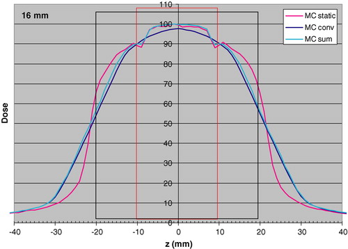
A presumption for the convolution method is that the calculated dose distribution will be invariant for small position changes. In a case like this with a solid tumor (unit density) in lung tissue, it may be expected that this is not a valid assumption. In order to check the validity of the convolution method, the longitudinal dose distribution was calculated by MC simulation through the centre of the 2 cm tumor and convolved with pdf (1,16). This dose distribution was compared to the one calculated with MC simulations by summing dose distributions obtained by displacing the beam on the long axis by −8 mm, −7 mm, … … . 7 mm, 8 mm. Each distribution had the same weight, to simulate a linear motion. In total 17 discrete dose distributions were added and weighted by 1/17, to simulate a linear motion. The result of this comparison is shown in Figure 2. As can be seen a significant difference appears close to the edge of the tumor, where the convolution method does not take the electron transport effects close to the border between the tissues correctly into account. At the center of the CTV the convolution underestimates the dose by 1.8%. This difference has, in the following been neglected, and the convolution method has been justified for the purpose of this work. In the same figure also the static MC simulated dose distribution is shown, for comparison.

Figure 2.  Longitudinal dose distributions obtained with MC simulations for the static case “MC static”; static MC convolved with the pdf (1,16) “MC conv”; linear sum of static MC obtained by displacements of the beam from −8 mm to +8 mm with one mm step “MC sum”. Calculations were made for a 2 cm tumor (red rectangle) with 1 cm margin (black rectangle). The dose 100 is 1.0 Gy for the PB algorithm to the centre of the target.

Results

All dose distributions shown in the figures are given as absolute dose. The value 100 represents a dose of 1 Gy to the centre of CTV, calculated with the PB algorithm.

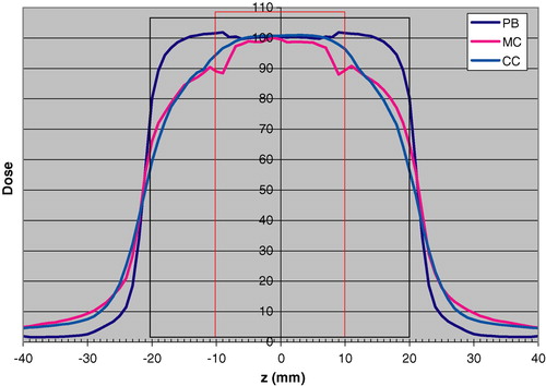
The static longitudinal dose distributions calculated with PB, CC and MC are shown in Figure 3 for the 2 cm tumor.

Figure 3.  Longitudinal dose distributions calculated for the static case respectively with the PB algorithm “PB”, MC simulation“MC” and the CC algorithm “CC”. The tumor diameter is 2 cm (red rectangle) and the margin size is 1 cm (black rectangle). The dose 100 is 1.0 Gy for the PB algorithm to the centre of the target.

In Figure 4a-d the probability distribution functions for the 10 mm amplitude are shown for the four different motion patterns.

Figure 4.  Probability density functions (pdf) for different motion patterns for 10 mm amplitude (peak to peak). In the figures the pdfs are for illustration purposes normalized to the maximum value of each pdf. a. Linear, fixed frequency and amplitude (pdf (1,10)). b. Harmonic oscillator fixed frequency and amplitude (pdf (2,10)).c. Pdf obtained from patient data [14] with fixed frequency and amplitude (pdf (3,10)). The right-hand side of the graph is the exhale phase. d. Pdf obtained from patient data [8] with variable frequency and amplitude. (pdf (4,10)). The right-hand side of the graph is the exhale phase.

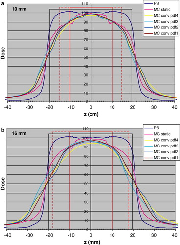
Figure 5 shows the results of the convolution of the MC calculated profiles with pdfs (1–4,10) (Figure 5a) and pdfs (1–4,16) (Figure 5b) for the 5 cm tumor. Figure 6 shows the corresponding data with pdfs (1–4,10) (Figure 6a) and pdfs (1–4,16) (Figure 6b) for the 2 cm tumor. For comparison, the static dose distribution calculated with the PB algorithm is also included in Figures 5 and 6.

Figure 5.  Longitudinal dose distributions obtained with the PB algorithm “PB”, with MC simulations for the static case “MC static” and static MC convolved respectively with pdf1 “MC conv pdf1”, pdf2 “MC conv pdf2”, pdf3 “MC conv pdf3” and pdf4 “MC conv pdf4”. The results are given for the 5 cm tumor (red rectangle) with 1 cm margin (black rectangle). The dotted red rectangle indicates the amplitude of 10 mm (Figure 5a) and 16 mm (Figure 5b). The dose 100 is 1.0 Gy for the PB algorithm to the centre of the target.

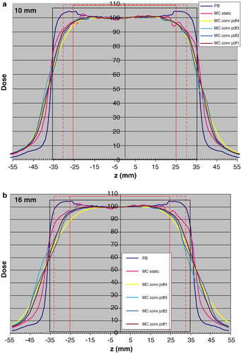
Figure 6.  Longitudinal dose distributions obtained with the PB algorithm “PB”, with MC simulations for the static case “MC static” and static MC convolved respectively with pdf1 “MC conv pdf1”, pdf2 “MC conv pdf2”, pdf3 “MC conv pdf3” and pdf4 “MC conv pdf4”. The results are given for the 2 cm tumor (red rectangle) with 1 cm margin (black rectangle). The dotted red rectangle indicates the amplitude of 10 mm (Figure 6a) and 16 mm (Figure 6b). The dose 100 is 1.0 Gy for the PB algorithm to the centre of the target.

Discussion

This work has focused on the comparison of dose distributions calculated by MC simulation with breathing motions included and the static dose distributions calculated in clinical treatment planning. The breathing motions are primarily in the longitudinal direction. For this reason only the longitudinal dose distribution through the center of the target has been studied in this paper, and parameters such as mean- and median doses to the targets are not meaningful to calculate from the longitudinal dose distributions calculated here.

The geometries of the phantom selected, as shown in Figure 1a, were chosen to be clinically relevant. The tumor sizes of 2 cm and 5 cm diameters, with a spherical shape of the GTVs, are representative for a small and a large GTV treated by SBRT at the Karolinska. To our knowledge, MC simulations of dose distributions for spherical GTVs located in lung tissue have not been presented before. The thicknesses of lung, upstream the tumors were, 5.5 cm and 4 cm. These dimensions were selected according to our 15 years of experience of SBRT of lung tumors, which are often located such that it is possible to select beam directions in such a way that only a moderate thickness of lung is included in the beam path to the target. The geometries were thus not selected to represent extreme cases, but more representative cases with proper selection of beam parameters. The geometries of the beams, shown in Figure 1b, are very representative for the PTVs chosen, except that in clinical practice, MLC collimation is used, instead of blocks. However, the important aspect of obtaining a heterogeneous dose distribution with beams smaller than the PTV in transverse direction is in agreement to clinical practice in SBRT.

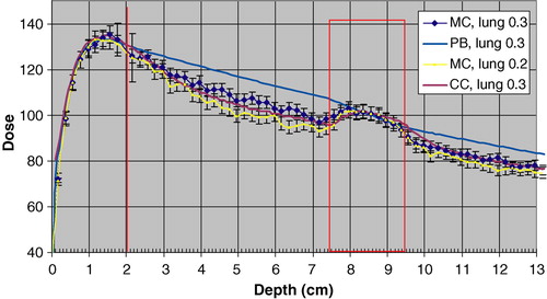
Another factor of importance, in this comparison of different ways to calculate dose, is the density of the lung. Here 0.3 g/cm³ was selected, which in some cases is representative, and in some cases may be an overestimation. To evaluate the impact of the lung density on the calculated dose distributions for this geometry, MC simulations were also done for a lung density of 0.2 g/cm³. Figure 7 shows the resulting depth dose, as well as calculated depth doses for a lung density of 0.3 g/cm³. As can be seen the dose to the centre of the CTV is the same as for a lung density of 0.3 g/cm³. The error bars shows two standard deviations.

Figure 7.  Depth Doses obtained with MC simulation, the PB algorithm and the CC algorithm for a lung density of 0.3 g/cm³. The MC calculated depth dose with a lung density of 0.2 g/cm³ is also depicted. The error bars show 2 SD. The dose 100 is 1.0 Gy for the PB algorithm to the centre of the target.

In this work it was assumed that the target and the lung tissues close to the target (where dose has been calculated) have the same motion pattern with the respiration. From the results (not published) of gated CT studies and MR studies at our hospital, this is a valid assumption. A second assumption that has been made is that the lung density is the same through the breathing cycle. In practice, the lung volume, and as a consequence the lung density is changing between inhale and exhale. This has been omitted in this work, as the breathing motions in clinical practice are controlled with the abdominal pressure, and in almost all cases kept within 10 mm.

Dose calculation in the static situation; PB and CC vs MC

From Figure 3, it can be seen that the dose to the GTV is estimated relatively accurately with the PB algorithm, except for the cranial and caudal interfaces to the lung tissue. The big difference is primarily in the volume between the GTV and PTV, with a considerable overestimation of the dose with the PB. Outside the PTV the situation is the reverse. The same results were obtained for the 5 cm CTV, although not shown here. With the CC algorithm, the agreement to the MC calculated dose is very good. The difference is primarily seen at the borders of the GTV, where the CC algorithm overestimates the dose.

As a check of the absolute dose calibration procedure in the MC simulations, an independent verification was made for a down stream slab geometry of 2 cm polystyrene, 5 cm of air and polystyrene. The slab geometry was selected because dosimetry is straightforward and accurate in this situation. Absolute dose was determined experimentally with an ionization chamber at 1.5 cm depth in the second polystyrene layer for both of the two beams in Figure 1b. The deviation between the MC dose (determined with the calibration procedure described in Material and Methods) and the measured one was 1.3% (MC dose, 2SD = 2.5%) for the 2 cm CTV beam and 1.8% (MC dose, 2 SD = 3.1%) for the 5 cm CTV beam. As a further verification of the calibration procedure, the depth dose curves for the beam of the 2 cm CTV shown in Figure 7 gives the same absolute dose (within the statistical uncertainty of the MC calculated dose) to the depth of dmax in the “chest wall”, as expected.

Dose calculation in the dynamic situation

As shown in Figure 2, the difference between the linear sum of MC calculated dose distributions and the convolution of the static MC distribution with the pdf (1, 16) is generally small. For the more realistic pdfs, the difference may be expected to be somewhat larger within the CTV. However, the 16 m amplitude represents an extreme value which is not representative for a clinical methodology in which abdominal compression is used to keep the motion to be within 10 mm. Thus the resulting dose distributions calculated by convolution for a 10 mm amplitude is expected to be accurate outside the CTV while within the CTV it underestimates the dose of the order of 2–5% and with the largest underestimation at the cranial and caudal borders of the CTV.

Effect of using different pdfs on the dose distribution

Figures 5 and 6 show that for the 10 mm amplitude, the differences between the different pdfs have a relatively minor effect on the dose distribution calculated by convolution. The pdf (4,10), including occasional deep breaths, may have a somewhat larger effect, compared to the other ones. The fact that pdfs 3 and 4 take into account that positions in the exhale phase are more likely than in the inhale phase has a minor effect on the dose distribution. More important is, as expected, the amplitude, given by the pdfs (1–4,16). For these situations, the differences in breathing motion pattern also will have a larger impact.

The largest differences seen from Figures 5 and 6 between the dose distributions calculated with the PB algorithm for the static case (used in clinical treatment planning) and convolved MC distributions are in the lung tissue between CTV and PTV (up to 30% or more), and to a smaller extent outside the PTV. Even though this paper only presents one dimensional dose distributions, it may be that the overestimation in dose by PB calculations between CTV and PTV is one important aspect related to the clinical finding that lung toxicity (contrary to what may be expected) is a minor clinical problem even when 15 Gy×3 is given to the periphery of the PTV within one week. The dose to the central part of the CTV is relatively accurately predicted by PB algorithms, however, with 10–15% overestimation at the periphery. It may be speculated that this is in accordance to clinical findings that the local control is generally reported to be very high at these fractions patterns.

Set-up reproducibility

In the results presented, the effect on the dose distribution of set-up errors has not been included. This cannot be simulated with a convolution method, especially for SBRT which are given with three fractions. However, a systematic and constant set-up error can easily be added to the breathing motions. In simulations we did of this, by summation of MC calculated longitudinal dose profiles for the 2 cm CTV case, with a constant set-up error of 3 mm in the longitudinal direction, and on top of that 10 mm breathing motions of the target, still results in a dose distribution to the CTV which is in close agreement to the one shown in Figure 2 (MC static). However, the dose to the volume between CTV and PTV will be more affected (results not presented here), and more asymmetric, than in the case of no set-up error.

Heterogeneous dose distribution in PTV and dose specification

The main advantage of using a heterogeneous dose distribution within the PTV was given above in the Introduction. This is related to the fact that for a multiple field technique, in which the beams are spread in a large solid angle, the relative dose to the volume outside of the PTV (normal tissue) is almost entirely given by the relative dose given to the periphery of the PTV [1], [3]. Thus, a higher relative dose to the central parts of the PTV, i.e. essentially the CTV will be a “bonus” with a consequently higher probability to kill the clonogenic tumor cells in the gross tumor. This argument is valid in SBRT of macroscopic solid tumors where the higher dose to the relatively small volume between CTV and PTV will be acceptable. The advantage mentioned here refers to a static situation.

A second advantage of using a heterogeneous dose distribution, with a higher relative dose in the center, refers to the dynamic situation. This includes both regular motions of the target due to respiration and random set-up errors. The higher dose inside the PTV will compensate the lower dose outside the PTV, when regular motions of the target relative to the beams are present, as in the clinical situation. In case of a homogeneous dose distribution within the PTV, no such compensation of dose will occur. In Figures 5 and 6 this compensation is clearly seen. The width of the 50% dose level is the same for the “MC static” and the convolved dose distributions. Interestingly and as expected, the PB algorithm gives almost the same width at the 50% level.

Several arguments may be raised regarding dose specification in SBRT when heterogeneous dose distributions are used. From the results given by Figures 5 and 6, it can be argued that the center of the target or the 50% level would be the relevant alternatives, considering both the dose computation errors in PB algorithms and the effect on the dose distribution from regular respiratory motions of the target. With the same arguments, dose levels at about 80 to 90%, which is commonly used, would be not such good alternatives for dose specification when PB algorithms are used. When a CC algorithm is used, the error in dose in far less, even though the difference between the dose distributions calculated for a static and a dynamic situation at the 80% dose level is considerable, as shown in Figures 5 and 6.

The primary aim of this work was to study the effect of breathing motions on the longitudinal dose distribution through the centre of a symmetrical target. From the results of this work it may be concluded that in many common clinical situations of SBRT of lung tumors, PB algorithms may give relatively good estimates of the dose to the GTV, but not for the lung volume outside the GTV. Thus for dose/volume correlations to toxicity data, PB algorithms are inferior, while the present results indicates that CC algorithms have a far higher accuracy. However, in order to draw further conclusions regarding accuracy requirements in the dose computation for correlation to biological effects of SBRT, 3D dose calculations are needed. This will also be needed in order to get reliable data for decisions on which situations respiratory gated SBRT of lung tumors will be needed and which situations a reduction of the respiratory motion with abdominal compression will be sufficient. A more thorough 3D analysis of dose distributions in SBRT of lung tumors is currently in progress.

Margins between CTV and PTV

One aim of this work was to see the effect on the dose distribution, given clinically relevant margins between CTV and PTV, when breathing motions are included. The question could however be turned to – does the results implicate something regarding requirement on margins? From Figure 5b and 6b it is seen that the there is a narrowing of the dose distribution, when breathing motions are included of about 20 mm compared to the static PB dose distribution at the 80–90% dose level. There is also a narrowing of the dose distribution compared to the static MC calculated one. From Figure 5a and 6a it may be concluded that the 10 mm margin is enough to give the same dose to the periphery of the CTV when breathing motions are included (assuming no set-up error), as for the static case, while with a 16 mm breathing amplitude, 10 mm margin is inadequate (cf Figure 5b and 6b). However, the question is difficult, as from clinical experience it is well known that the local control in SBRT of lung tumors is generally high, and the local recurrences that appear may have several causes. One is that the prescribed dose was inadequate another that the margins were inadequate and a third that the target definition was inadequate, or some combination of the three. Preferably, breathing motions, as well as set-up errors should ideally be included in the dose distributions calculated in clinical treatment planning.

Conclusions

This work deals with calculated dose distributions in the longitudinal direction through the center of spherical tumors (2 cm and 5 cm diameter) in a lung phantom. Respiratory motions of the tumors were included in the calculations.

In the static situation, the collapsed-cone algorithm gives a good agreement to the Monte-Carlo calculated distributions within and outside of the GTV. Compared to Monte-Carlo, the pencil beam algorithm overestimates the dose up to 30% outside the GTV and overestimates the dose up to 10% within the GTV.

For the dynamic situation convolution was used of different respiratory motion patterns with the MC calculated dose distribution. The use of the convolution method in lung tumors was validated. In the comparison between the pencil beam static situation (used in clinical dose planning) and the dynamic situation (which takes the respiratory motion into account), a narrowing of the latter dose distribution of about 20 mm at the 80–90% dose level is seen, for a motion amplitude of 16 mm.

This work was supported by grants from the Cancer Society in Stockholm.

References

- Lax I, Blomgren H, Näslund I, Svanström R. Stereotactic radiotherapy of malignancies in the abdomen. Methodological aspects. Acta Oncol 1994; 33: 677–83
- Lax I, Blomgren H, Larson D, Näslund I. Extracranial stereotactic radiosurgery of localized targets. J Radiosurg 1998; 1: 63–74
- Lax I. Target dose versus extra target dose in stereotactic radiosurgery. Acta Oncol 1993; 32: 453–7
- Kavanagh BD, Timmerman RD. Stereotactic body radiation therapy. Lippincott Williams & Wilkins, Philadelphia 2005
- Lujan AE, Larsen E, Balter JM, Ten Haken R. A method for incorporating organ motion due to breathing into 3D dose calculations. Med Phys 1999; 26: 715–20
- Beckham WA, Keall PJ, Siebers JV. A fluence convolution method to calculate radiation therapy dose distributions that incorporate random set-up error. Phys Med Biol 2002; 47: 3465–73
- Chetty I, Rosu M, McShan D, Fraass B, Balter J, Ten Haken R. Accounting for center-of-mass target motion using convolution methods in Monte-Carlo based dose calculations of the lung. Med Phys 2004; 31: 925–32
- George G, Vedam SS, Chung TD, Ramakrishnan V, Keall PJ. The application of sinusoidal model to lung cancer patient respiratory motion. Med Phys 2005; 32: 2850–61
- Salvat F, Fernandez-Varea J M, Sempau J. 2003 PENELOPE, A code system for Monte Carlo simulation of electron and photon transport (Issy-les-MoulineauxFrance: OECD Nuclear Energy Agency) ( Available in PDF format at http://www.nea.fr).
- Badano A, Sempau J. MANTIS: Xray, electron and optical Monte Carlo simulations of indirect radiations imaging systems. Phys Med Biol 2006; 51: 1545–61
- Sempau J, Andreo P, Aldana J, Mazurier J, Salvat F. Electron beam quality correction factors for plane-parallel ionization chambers: Monte Carlo calculations using the PENELOPE system. Phys Med Biol 2004; 49: 4427–44
- Fraas B, Doppke K, Hunt M. Quality assurance for clinical radiotherapy treatment planning. AAPM Radiation Therapy committee TG53. Med Phys 1998; 25: 1773–1829
- Ma CM, Price RA, Li JS, Chen L, Wang L, Fourkal E, et al. Monitor unit calculation for Monte Carlo treatment planning. Phys Med Biol 2004; 49: 1671–87
- Ford EC, Mageras GS, Yorke E, Rosenzweig KE, Wagman R, Ling CC. Evaluation of respiratory movement during gated radiotherapy using film and electronic portal imaging. Int J Radiat Oncol Biol Phys 2002; 52: 522–31