Optimal treatment margins for radiotherapy of prostate cancer based on interfraction imaging

Abstract

Purpose. To present a methodology to estimate optimal treatment margins for radiotherapy of prostate cancer based on interfraction imaging. Materials and methods. Cone beam CT images of a prostate cancer patient undergoing fractionated radiotherapy were acquired at all treatment sessions. The clinical target volume (CTV) and organs at risk (OARs; bladder and rectum) were delineated in the images. Random sampling from the CTV-OAR library was performed in order to simulate fractionated radiotherapy including intra- and interpatient variability in setup and organ motion/deformation. For each simulated patient, four treatment fields defined by multileaf collimators were automatically generated around the planning CTV. The treatment margin (the distance from the CTV to the field border) was varied between 2.5 and 20mm. Resulting dose distributions were calculated by a convolution method. Doses to OARs were reconstructed by polynomial warping, while the CTV was assumed to be a rigid body. The equivalent uniform dose (EUD), the tumor control probability (TCP) and the normal tissue complication probability (NTCP) were used to estimate the clinical effect. Patient repositioning strategies at treatment were compared. Results. The simulations produced population based EUD histograms for the CTV and the OARs. The number of patients receiving an optimal target EUD increased with increasing margins, but at the cost of an increasing number receiving a high EUD to the OARs. Calculations of the probability of complication-free tumor control and subsequent analysis gave an optimal treatment margin of about 10mm for the simulated population, if no correction strategy was undertaken. Conclusions. The current work illustrates the principle of optimal treatment margins based on interfraction imaging. Clinically applicable margins may be obtained if a large patient image database is available.

Geometrical uncertainties in external beam radiotherapy stem from a variety of sources; for instance, tumor delineation, organ motion, and patient-beam setup [1]. Such uncertainties pose problems, as healthy tissue must be included in the treated volume in order to maximize tumor cell eradication. Organs at risk (OARs) may thus receive intolerable radiation doses.

Formally, geometrical uncertainties may be taken into account by introducing treatment margins, resulting in a Planning Target Volume (PTV) and a Planning organ at Risk Volume (PRV) [2]. Based on population uncertainty analyses, margin recipes for both the PTV and PRV have been presented [3], [4]. However, it is not straightforward to handle PRVs overlapping the PTV in radiotherapy planning [5]. By incorporating spatial coverage probabilities into cost functions for optimizing Intensity Modulated RadioTherapy (IMRT), this issue has partly been overcome [6]. Yet, tumor and organ motion may be correlated, complicating such calculations.

Cone Beam Computed Tomography (CBCT) at treatment [7] is useful for estimating geometrical setup errors, and may be employed for 3D correction strategies of patient setup [8], [9]. The aim of such strategies may be to reduce normal tissue toxicity while maintaining the prescribed tumor dose, or to boost the tumor to a higher dose while keeping the normal tissue toxicity at an acceptable level. In any case, the strategies imply that smaller treatment margins should be used.

The evaluation of radiotherapy treatments, even when based on multiple image sets acquired during a fractionated treatment course, is complicated by variable patient anatomy. The key problem is to keep track of accumulated doses in each tissue element [10], [11]. Especially for organs at risk showing a serial tissue architecture with respect to radiosensitivity, dose tracking is warranted.

In the current work, we have studied the effect of given treatment margins on a simulated population receiving conformal radiotherapy. An automated treatment planning, dose calculation and dose tracking engine was developed to estimate the clinical effect on a population level based on multi-patient, multi-image information. Systematic and random errors from patient beam setup, tumor motion and organ deformation were implicitly included. Different correction strategies were discussed.

Materials and methods

Patient data

CT imaging and organ delineation

CT images with 2.5 mm slice thickness and 0.92 mm pixel resolution of a prostate cancer patient were acquired using a GE Lightspeed Ultra scanner (140 kV; GE Healthcare, UK). Both the length and diameter of the field of view was about 25 cm. The images were transferred to the Oncentra MasterPlan v.3.0 (Nucletron, The Netherlands) treatment planning system, where the gross tumour volume, the bladder and the rectum were delineated. The clinical target volume (CTV) was generated by adding a 5 mm isotropic margin to the GTV.

Treatment and CBCT imaging

The patient received a sequential treatment, where first the prostate and the seminal vesicles were treated to 50 Gy in 25 fractions. Then, the prostate was given 24 Gy in 12 fractions. The treatment was carried out at an Elekta Synergy linear accelerator (Elekta, UK) using four conformal 15 MV photon beams. Following patient alignment according to skin marks, cone beam CT images were acquired using the XVI CBCT system (120 kV; Elekta, UK) before treatment delivery. The reconstructed CBCT slice thickness was 3 mm, with 1 mm pixel resolution. The length and diameter of the field of view was about 12 and 40 cm, respectively. Images were acquired at all 37 treatment fractions. CT and CBCT images were coregistered by minimizing the correlation coefficient between bone segmented CT and CBCT images, and the setup error at a given treatment fraction could thus be estimated. The rectum and bladder was manually delineated in all image series.

Prostate fiducial markers

Prior to imaging and treatment, three Goldlock III markers (Beampoint AB, Sweden) with dimensions 0.8×0.8×3 mm were transrectally implanted in the prostate by a urologist. Using software developed in-house, the gold markers were automatically detected in the CT and CBCT images. The uncertainty in the measured marker position was estimated to 0.3, 0.6 and 0.6 mm in the medial-lateral, cranial-caudal and anterior-posterior direction, respectively. The prostate position was estimated from the mean position of the markers. Following CT and CBCT coregistration, the prostate position within the bony anatomy at a given treatment fraction was estimated.

Patient population simulations

In the current work, the treatment margin is defined as the distance from the CTV to the field border. The margin was isotropic. As the effect of a given margin on a patient population was to be simulated, an automated set of tools for handling multi-patient, multi-image data was developed in-house.

Patient population

The image data base was constituted by 38 (1 CT and 37 CBCT) image series, where series 1 corresponded to the CT images, while series 2 were obtained by CBCT at the first treatment fraction, etc. Random sampling (with replacement) from the image data base was performed. Briefly, for a given simulated patient, a random number between 1 and 38 was drawn. The image series corresponding to that random number was then used as planning basis for the treatment. Treatment images were generated by drawing another 37 random numbers, and selecting corresponding image series from the database. 1 000 patient histories were generated by this procedure.

For each simulated patient and treatment margin, a full 3D dose distribution based on the given planning images was generated from a four-field treatment plan as outlined below. Uncertainties due to tumor and organ delineation were taken into account by convoluting the dose distribution with an isotropic Gaussian of 3 mm width. The dose to the prostate and the OARs was then scored in the randomly selected anatomy found at treatment, and the cumulative dose was calculated using dose tracking procedures (see below).

Dose computation

For a given margin, the patient dose distribution was calculated using a convolution method. Briefly, four equispaced 15 MV photon beams defined by multi-leaf collimators were generated around the planning CTV. The beam weights were 100, 60, 30, and 60 for the beams at 0, 90, 180 and 270° gantry angle, respectively, which from our clinical experience is expected to give satisfactory target coverage with tolerable doses to the OARs. Beam divergence was disregarded. The MLC leaf width was 1 cm at the isocenter. The leafs were positioned in an “out-of-field” configuration, where, in beams-eye-view projection, the closest distance from the leaf tip to the CTV contour was defined by the specified treatment margin. The shaped photon beams were exponentially attenuated within the patient. The dose distribution was obtained by convolving the photon intensity distribution in the patient with a 3D anisotropic Gaussian scatter kernel. The scatter kernel and the linear attenuation coefficient were adjusted so that the resulting 3D dose distribution was similar to that found from measurements of 15 MV photons (, penumbra width 4 mm) in a water phantom. No inhomogeneity corrections were applied. The sequential treatment outlined above was followed, with a mean total dose to the CTV of 74 Gy. The dose distributions in the CTV and OARs were similar to those obtained from comparable four-field treatment plans generated in the MasterPlan treatment planning system (data not shown).

Dose tracking

In the following, procedures for tracking the absorbed dose in given voxels of a reference image basis are presented. In the planning image basis, which serves as a reference, the set of voxels constituting a volume of interest (VOI) is denoted (X₀, Y₀, Z₀). In the image basis obtained at treatment fraction n, the VOI is defined by (X_n, Y_n, Z_n). We seek three geometric transformation functions f, g and h so that X_n=f(X₀, Y₀, Z₀), Y_n=g(X₀, Y₀, Z₀) and Z_n=h(X₀, Y₀, Z₀). The warped dose distribution at a given treatment fraction in the reference VOI, as obtained from the geometric relation between the two sets of coordinates, is thus given by:1 where D_n is the dose distribution in the patient at treatment fraction n.

The prostate was assumed to be a rigid body. Rotations were omitted. At a given treatment fraction, the position of the prostate, as delineated in the planning CT images, was found by calculating the mean position of the fiducials. Denoting the distance between the prostate positions at planning and treatment imaging (Δx, Δy, Δz), the geometric transformation is given by a simple translation: (X_n, Y_n, Z_n)=(X₀+Δx, Y₀+Vy, Z0 + Vz).

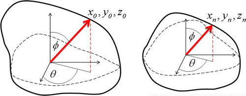
For the OARs, experiencing interfraction deformations, polynomial image warping was performed. In polynomial warping, a set of corresponding control points (landmarks; see below) in the planning and treatment image set are needed in order to obtain the appropriate geometric transformation. For the bladder, three-dimensional warping was performed. It was assumed that the set of control points in the treatment image is transformed according to the polynomial:2 The coefficients P_i,j,k that maps (X₀, Y₀, Z₀) into X_n was found by least squares linear regression. The procedure was repeated for Y_n and Z_n. For the bladder, the control points were found by first identifying the geometric center of the bladder in the planning and treatment image basis, respectively. Then, 2 000 lines were extended from the geometric center to the bladder wall at varying solid angles. The intersection of the lines with the bladder wall defined the control points (Figure 1). Thus, 2 000 control points were used in the polynomial regression procedure (Equation 2).

Figure 1.  Definition of control points for the three-dimensional polynomial warping procedure for reconstructing bladder doses. To the left, the reference bladder is shown. The origin of the coordinate system is found in the center of mass. For a given solid angle, defined by θ and φ, a radial line is extended from the origin to the bladder wall, where the intersection defines a control point (x₀, y₀, z₀). The same procedure is performed for the bladder at treatment fraction n (right).

As the delineated rectum is not a closed organ, two-dimensional polynomial warping was performed slice-by-slice in the axial images. Thus, a variant of Equation 2 was used, where terms involving Z were omitted. As for the bladder, the geometric center of the axial rectum contour was found, and lines were extended from the center to the wall. A total of 3 000 control points were used.

Biological effect

The generalized equivalent uniform dose (EUD), the tumor control probability (TCP) and the normal tissue complication probability (NTCP) were used to evaluate a given dose distribution. For the EUD, ‘a’ values of −24, 2.3, and 10 were used for the prostate [12], bladder [13], and rectum [14], respectively. For TCP calculations, the linear quadratic Possion cure model, including interpatient variation in cellular radiosensitivity, was used [15]. For this model, the linear and quadratic terms were α=0.15 Gy⁻¹ and β=0.05 Gy⁻² [16]. The total number of clonogens was set to 10⁷ [16]. By manual iteration, an interpatient standard deviation in α of 0.03 Gy⁻¹ gave a TCP which agreed well with data for local control [17]. For the NTCP, an EUD-based model, with a logistic response function, was used [18]. In this case, tolerance data from Emami et al. [19] where fitted to the response function in order to estimate the logistic parameters. Finally, the probability of complication free tumor control was calculated according to [20]:3

Correction strategies

Three different correction strategies were compared: (1) no corrections, (2) correcting for patient setup at every treatment fraction using bone matching (“bone match”) and (3) correcting for prostate position at every treatment fraction using the gold markers (“prostate match”).

Software

All image analyses and simulations were performed with the Interactive Data Language v.6.0 (IDL; ITT Visual Information Solutions, USA).

Results

Patient data

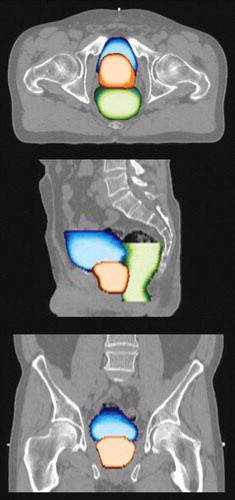
The random setup error for the patient in question was 1.4, 1.3, and 2.5 mm in the medial-lateral, cranial-caudal and anterior-posterior direction, respectively, while the random prostate displacement was 0.4, 1.3 and 1.6 mm, respectively. The tumor volume at start of treatment was 85 cm³. Using the mean distance between the markers, the tumor volume at each treatment fraction was estimated. Subsequent linear regression showed that the tumor shrunk insignificantly during treatment (p = 0.14). The mean volume±standard deviation of the bladder and rectum was 190±35 and 160±20 cm³, respectively. The correlation coefficient between the prostate displacement and rectum volume was 0.45 (p = 0.005), while it was 0.16 (p = 0.33) between the prostate and the bladder. In Figure 2, the spatial probability distribution (the coverage probability), as derived from all 38 imaging sessions, of the prostate, bladder and rectum within the bony anatomy is superimposed on the planning CT image basis.

Figure 2.  Illustration of the spatial probability distribution of the prostate (orange), rectum (green) and bladder (blue) taken over the fractionated treatment. Bright colors indicate a high probability. The top, middle and lower image correspond to the axial, sagittal and coronal plane, respectively.

Patient simulations

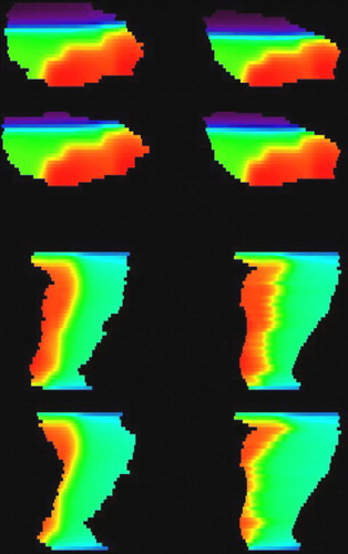
From the dose calculation engine developed, the patient dose distribution based on one of the 38 image sets is shown in Figure 3. As apparent, clinically relevant, conformal dose distributions were generated. The standard deviation in CTV dose was within 2% for margins equal to or greater than 7.5 mm (data not shown). The dose distribution in the bladder and rectum at two different treatment fractions is shown to the left in Figure 4. Note the coarse MLC pattern in the bladder and the interfraction variations in organ shape. In Figure 4, to the right, the warped dose distribution in the reference OAR is shown. The polynomial warping results in a modulation of the original dose distribution, but the main features are well reflected.

Figure 3.  Computed patient dose distribution in the axial (top), sagittal (middle) and coronal (bottom) plane, respectively. For clarity, only the CTV and the external patient contour are shown. A treatment margin of 10 mm was used. Notice the MLC field shaping.

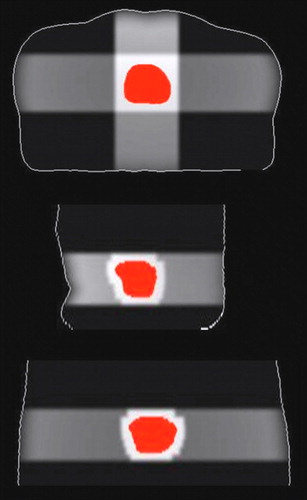
Figure 4.  Dose images in the sagittal plane for the bladder (top four) and rectum (bottom four). To the left are to dose distributions generated in organs delineated in cone beam CT images, while to the right are corresponding warped dose distributions in the reference organ.

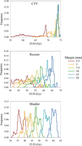
Following dose planning and dose tracking for the 1 000 simulated patients, resulting EUD distributions for the tumor and OARs are shown in Figure 5. In this case, no correction strategy was employed. As apparent from the width of the respective distributions, rather large interpatient variations in EUD were found. Furthermore, the median EUD was increased, while the width of the distribution was reduced with increasing margin for both the tumor and the OARs. These features were present regardless of correction strategy (data not shown).

Figure 5.  Dependence of simulated population-based EUD histograms for the CTV (top), rectum (middle) and bladder (bottom) on the treatment margin. In this case, no correction strategy was employed. Note the varying abscissa and ordinate scaling.

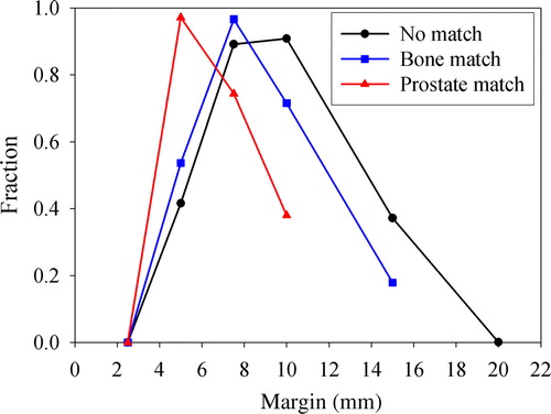
The EUD histograms were further analyzed. Reasonable ad hoc criteria for accepting a dose plan with a given treatment margin is that the EUD to an OAR is lower than the tolerance dose for 5% complication probability, while the EUD to the CTV is greater than 98% of the prescribed dose (74 Gy). Using tolerance doses from Emami et al. [19], being 60 Gy for severe rectal proctitis/necrosis/fistula/stenosis and 65 Gy for symptomatic contracture and volume loss of the bladder, the dependence of the fraction of patients fulfilling the criteria on the treatment margin was obtained (Figure 6). As apparent, the fraction of patients fulfilling the criteria rises to a maximum before it declines to zero at large margins. The optimal margin was 10, 7.5 and 5 mm following no corrections, correcting for patient setup and correcting for prostate displacement, respectively. The latter showed the narrowest margin interval where a significant fraction (e.g. 50%) fulfilled the criteria.

Figure 6.  Dependence of the fraction of patients fulfilling EUD-based criteria on the treatment margin, for different correction strategies. The criteria were that the relative difference between the prescribed dose and EUD_CTV could not exceed 2%, while EUD_OAR could not exceed the tolerance dose for 5% complication probability.

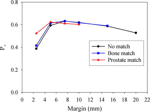
In Figure 7, the dependence of the population-based TCP and NTCP on the treatment margin is shown. TCP increases to a maximum level of about 0.9, while NTCP for the rectum and bladder increases sigmoidally with increasing margin. As apparent, correcting for prostate motion yields a TCP of about 0.55 for the smallest margin (2.5 mm), being nearly 15 percentage points higher than if no corrections were performed. Correcting for prostate motion also increased the NTCP for the rectum, while this had little or no effect on the bladder. These findings are condensed into Figure 8, where the P₊ is plotted against treatment margin. P₊ is seen to increase to a maximum with increasing margin before a slow decline is observed. The optimal margin was in this case 7.5, 7.5 and 5 mm following no corrections, correcting for patient setup and correcting for prostate displacement, respectively. For the latter, using a margin of only 2.5 mm, a near optimum P₊ was obtained.

Figure 7.  Dependence of the tumor control probability (TCP) and the normal tissue complication probability (NTCP) on the treatment margin, for different correction strategies.

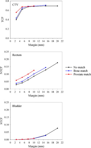
Figure 8.  Dependence of the probability of complication free tumor control (P₊) on the treatment margin, for different correction strategies.

Discussion

The current work shows that optimal treatment margins may be derived from multi-patient, multi-image data. Depending on the biological indices chosen for evaluating the clinical effect (EUD, P₊), the margins may be considered the best compromise between tumor cell eradication and normal tissue toxicity. The present work also illustrates the effect of two different correction strategies. It is emphasized that the optimal margins derived from the simulated population are mainly of qualitative interest and should not be employed in the clinic.

The random setup error and interfraction prostate displacement for the current patient agrees well with previously published findings for prostate cancer patients [3]. The prostate displacement correlated significantly with rectal filling, while an insignificant correlation was found with bladder filling, which is in line with previous findings [21]. This confirms the relevance of the patient data employed in the current simulations.

Dose tracking (or dose reconstruction) is important for accurate evaluation of radiotherapy. Many different reconstruction algorithms have been proposed (see [10] and references therein). In the current work, as a first step to introduce dose reconstruction, polynomial warping was employed. In this case, the treatment OAR, relative to the planning OAR, was assumed to be stretched or shrunk along radial lines from the geometric centre. The degree of stretching is contained in the polynomial coefficients (Equation 2). The polynomial warping resulted in reasonable reconstructed dose distributions in the reference organs (Figure 4). It is not expected that other reconstruction methods would have changed the main conclusions of the current study.

The random sampling procedure produced a patient population suitable for evaluating the effect of a given margin. Due to the complexity of the calculations, some further limitations were introduced. First, prostate rotation was disregarded in the simulations. Prostate rotation has a rather low impact on population-based TCP calculations for given treatment margins [3]. Second, intra-fraction prostate motion, likely to be much smaller than inter-fraction displacement, was considered negligible, as other error sources dominate. Third, inclusion of other organs at risk, e.g. the small intestine and the femoral heads, may influence the results. Fourth, only isotropic margins were used. As the current patient showed quite anisotropic random setup errors and prostate displacements, the isotropic margins represent spatial compromises. Fifth, the findings are confined to the currently used four-beam setup, and other beam configurations may give different results.

In the current work, optimal margins were derived from either EUD or P₊. In the case of EUD, a comparable approach has been presented previously [22]. In that work, geometric uncertainties were evaluated in a cubic phantom containing a spherical CTV and OAR. Also, emphasis was on investigating margin reduction alongside an increase in the isocenter dose. In our work, the mean dose to the CTV was constant (74 Gy).

The population based EUD histograms (Figure 5) illustrate that quite large interpatient variations in treatment response may be expected, especially for the OARs, which are solely due to geometric uncertainties. By introducing EUD-based criteria, the number of patients fulfilling the criteria typically followed a bell-shaped curve (Figure 6). The curve shape is due to that for small margins, few patients have an EUD_CTV greater than 98% of the prescribed dose, while for large margins, few patients presented an EUD_OAR less than the 5% tolerance dose. However, the endpoints selected for the OARs were severe complications [19]. By requiring less severe complications, the tolerance dose should be lowered. In this case, the bell-shaped curve (Figure 6) may be contracted and the optimal margin may be reduced. The histogram analysis method proposed here is quite attractive, as the clinician may interactively change the EUD-based tolerance levels and directly evaluate the effect of different margins.

As an alternative to EUD-based margins, which depend on selected tolerance levels, TCP and NTCP were estimated (Figure 7), resulting in an objective P₊ (Figure 8). As the probability of including the CTV or the OARs within the treatment beams increase with increasing margin, both the TCP and the NTCP increase. The resulting P₊ curve was concave, but to a lesser extent than for the fraction of patients fulfilling the EUD-based criteria. Thus, from the P₊ calculations, it appears that the effect of a margin reduction or increase is not that pronounced compared to that what was obtained from the EUD calculations. This is most likely due to that P₊ may be considered to implicitly include interpatient blurring of the EUD distribution by the TCP and NTCP response functions.

Three different strategies with respect to patient repositioning at treatment were compared in the current work. In the first approach, the simulated population was treated without any corrections. Based on TCP calculations, van Herk et al. [3] have provided a general CTV-PTV margin recipe: 2.5Σ + 0.7σ, where Σ and σ is the systematic and random error, respectively. For our simulated population (based on random sampling from one patient image database), the systematic setup error was equal to the random setup error. This was also the case for the prostate displacement. Using an isotropic organ delineation error of 3 mm, the margin recipe, including 3 mm from the PTV to the field border, gave 12, 13 and 16 mm in the medial-lateral, cranio-caudal and anterior-posterior direction, respectively. Our optimal margins, albeit isotropic, were around 7.5–10 mm, depending on which of the biological indices to be used. Although our optimal margins and the margins derived from the TCP-based margin recipe [3] are not directly comparable due to e.g. different modeling approaches and scoring criteria, this indicates that margins should be reduced if normal tissue damage is taken into account.

By comparing the three different correction strategies (Figures 6–8), it appears that image coregistration at the time of treatment with subsequent correction of patient positioning implies using smaller margins, as could have been expected. Furthermore, Figure 7 indicates that if setup corrections are performed at treatment while employing margins for non-corrected strategies, increased normal tissue injury to the rectum may result. Also, for a given margin, a slight increase in normal tissue damage to the rectum is observed following application of correction protocols. This was especially the case when correcting for prostate displacement. The increase in NTCP is due to that a correction implies moving the organ to a more reproducible position if the matching structure (e.g. the prostate) correlates with motion/deformation of the OAR. The maximum accumulated dose in a tissue element is thus expected to increase, thereby increasing NTCP for organs predominantly showing a serial architecture. This is the case for the rectum.

The current work was limited by the restricted amount of image data available. A future study is planned where a larger patient cohort is to be evaluated.

Acknowledgements

Discussions with Professor Dag Rune Olsen and medical physicist Jan Rødal are gratefully acknowledged.

References

- van Herk M. Errors and margins in radiotherapy. Semin Radiat Oncol 2004; 14: 52–64
- ICRU. Report 62: Prescribing, recording and reporting photon beam therapy ( supplement to ICRU report 50), 1999.
- van Herk M, Remeijer P, Lebesque JV. Inclusion of geometric uncertainties in treatment plan evaluation. Int J Radiat Oncol Biol Phys 2002; 52: 1407–22
- McKenzie A, van Herk M, Mijnheer B. Margins for geometric uncertainty around organs at risk in radiotherapy. Radiother Oncol 2002; 62: 299–307
- Goitein M. Organ and tumor motion: An overview. Semin Radiat Oncol 2004; 14: 2–9
- Jaffray DA, Siewerdsen JH, Wong JW, Martinez AA. Flat-panel cone-beam computed tomography for image-guided radiation therapy. Int J Radiat Oncol Biol Phys 2002; 53: 1337–49
- Nuver TT, Hoogeman MS, Remeijer P, van Herk M, Lebesque JV. An adaptive off-line procedure for radiotherapy of prostate cancer. Int J Radiat Oncol Biol Phys 2007; 67: 1559–67
- Nijkamp J, Pos FJ, Nuver TT, De Jong R, Remeijer P, Sonke JJ, et al. Adaptive radiotherapy for prostate cancer using kilovoltage cone-beam computed tomography: First clinical results. Int J Radiat Oncol Biol Phys 2008; 70: 75–82
- Zhong HL, Weiss E, Siebers JV. Assessment of dose reconstruction errors in image-guided radiation therapy. Phys Med Biol 2008; 53: 719–36
- Schaly B, Kempe JA, Bauman GS, Battista JJ, Van Dyk J. Tracking the dose distribution in radiation therapy by accounting for variable anatomy. Phys Med Biol 2004; 49: 791–805
- Sovik A, Ovrum J, Olsen DR, Malinen E. On the parameter describing the generalised equivalent uniform dose (gEUD) for tumours. Physica Medica 2007; 23: 100–6
- Malinen E, Lervag C, Soevik A. Ranking of treatment plans by the equivalent uniform dose including model uncertainties. Radiother Oncol 2007; 84: S280–S281
- Ghilezan M, Yan D, Liang J, Jaffray D, Wong J, Martinez A. Online image-guided intensity-modulated radiotherapy for prostate cancer: How much improvement can we expect? A theoretical assessment of clinical benefits and potential dose escalation by improving precision and accuracy of radiation delivery. Int J Radiat Oncol Biol Phys 2004; 60: 1602–10
- Nahum AE, Sanchez-Nieto B. Tumour control probability modelling: Basic principles and applications in treatment planning. Physica Medica 2001; 17: 13–23
- Wang JZ, Guerrero M, Li XA. How low is the alpha/beta ratio for prostate cancer?. Int J Radiat Oncol Biol Phys 2003; 55: 194–203
- Fowler J, Chappell R, Ritter M. Is alpha/beta for prostate tumors really low?. Int J Radiat Oncol Biol Phys 2001; 50: 1021–31
- Gay HA, Niemierko A. A free program for calculating EUD-based NTCP and TCP in external beam radiotherapy. Physica Medica 2007; 23: 115–25
- Emami B, Lyman J, Brown A, Coia L, Goitein M, Munzenrider JE, et al. Tolerance of normal tissue to therapeutic irradiation. Int J Radiat Oncol Biol Phys 1991; 21: 109–22
- Kallman P, Lind BK, Brahme A. An algorithm for maximizing the probability of complication-free tumor-control in radiation-therapy. Phys Med Biol 1992; 37: 871–90
- van Herk M, Bruce A, Kroes APG, Shouman T, Touw A, Lebesque JV. Quantification of organ motion during conformal radiotherapy of the prostate by three dimensional image registration. Int J Radiat Oncol Biol Phys 1995; 33: 1311–20
- Song W, Dunscombe P. EUD-based margin selection in the presence of set-up uncertainties. Med Phys 2004; 31: 849–59