A simulation of MRI based dose calculations on the basis of radiotherapy planning CT images

Abstract

Background. The advantage of MRI-based radiotherapy planning is the superior soft tissue differentiation. However, for accurate patient dose calculations, a conversion of the MR images into Hounsfield CT maps is necessary. The aim of the present study was to investigate the dose accuracy that can be achieved with segmented MR-images derived from the planning CT images by assigning fixed densities to different classes of tissues. Methods. Treatment plans for ten prostate cancer patients were selected. A collapsed cone algorithm was used to calculate patient dose distributions. The dose calculations were based on four different image sets: (1) the original CT-series (DD_DP), (2) a simulated MR series with all tissue set to a homogenous water equivalent material of density 1.02 g/cm³ (DD_W), (3) a simulated MR series with soft tissue set to a water equivalent material with density 1.02 g/cm³ and the bone set to a density of 1.3 g/cm³ (DD_W+B1.3), and (4) a simulated MR series identical to (3) but with a bone density equal to 2.1 g/cm³ (DD_W+B2.1). The dose distributions were compared by analysing dose difference histograms as well as through a visual display of spatial dose deviations. Results. The population based minimum, mean and maximum dose difference between the DD_DP and DD_W in the target volume was −2.8, −1.0 and 0.6%, respectively. Corresponding differences between DD_DP and DD_W+B1.3 were −1.6, 0.2 and 1.5%, respectively, and between DD_DP and DD_W+B2.1 −4.3, 4.2 and 9.7%, respectively. For the rectum, the differences between CT_DP and the other image sets were in the range of −19.5 to 8.8%. For the bladder, the differences were in the range of −9.6 to 7.0%. Conclusions. A systematic study using segmented MR images was undertaken. To achieve an acceptable accuracy in the CTV dose, the MR images should be segmented into bone and water equivalent tissue. Still, significant dose deviation for the organs at risk may be present. As tissue segmentation in real MR images is introduced, segmentation errors and errors that stem from geometrical non-linearities may further reduce the accuracy.

Magnetic resonance (MR) imaging provides superior soft tissue contrast compared to computer tomography (CT) images, facilitating precise delineation of target volumes and organs at risk [1–4]. MR imaging is thus in many cases a prerequisite for the design of highly conformal treatments that involve an escalation of dose, and where a reduction of treatment margins is required to avoid unacceptable toxicity levels. Recent papers have addressed the sole use of MR images for treatment planning of external beam radiotherapy [5–11]. In developing this strategy, it is among others important to address limitations arising from dose calculations based on MR images that are converted into images containing a limited range of tissue densities.

The lack of tissue density information in the MR images hinders the direct use of these images for dose calculations. In addition, non-linearities in the magnetic field give rise to geometrical inaccuracies that limit the accuracy of beam delivery to the patient. These effects were addressed in detail in an early review by Khoo et al. [12]. They concluded that the use of MR images as the sole basis for treatment planning was premature among other reasons due to a lack of proper tools and methods to evaluate the impact of the above mentioned short comings, and further investigations were needed.

A first order approach in the use of MR images for planning is simply to ignore tissue inhomogeneities as such, and assign a bulk density equal to 1.0 g/cm³ to the entire body volume. The influence of this approach on the calculation of dose distributions has been investigated for treatment planning of prostate cancer and brain tumors [6], [7], [10], [11]. These authors have argued that the use of a homogenous tissue density have negligible dosimetric impact on the calculated dose compared to using full CT tissue density information in the dose calculations. They have consequently used a homogenous geometry in the planning images as the basis for further dosimetric evaluations of MRI-based treatment plans. Lee et al. [8] and Kristensen et al. [9] have however performed more in depth investigations of the dosimetric effects of reducing tissue heterogeneity, by introducing a second tissue class in addition to water, i.e. bone, for radiation treatment planning of prostate cancer and brain tumors, respectively. The results of these investigations implied that by completely ignoring tissue heterogeneity, significant dose differences may occur. Lee et al. reported dose discrepancies for the planning target volume mostly greater than 2%, ranging from 0–5% in the high dose-regions. Likewise, Kristensen et al. reported dose errors greater than 2% in low dose areas when planning on homogenous tissue geometry only.

Traditionally, problems related to MR image distortions from non-linearities in the magnetic fields, have been overcome through image registration and subsequent fusion of the MR images with the planning CT images [1–4], [13]. It is argued by Fransson et al. [13] that these geometric distortions may introduce errors in the definition of the target volumes that are not yet fully evaluated. Furthermore, these errors make a point by point comparison of the CT- and MR-based dose distributions difficult.

To use the MR images as a sole basis of radiation treatment planning, tissues must be segmented into different classes and assigned a tissue density or Hounsfield Unit value. However, tissue segmentation in MR images is all but trivial. It is therefore important to examine to what level the tissue classification needs to be taken, and subsequently what tissue densities to apply, in order to attain clinically acceptable dose distributions. The aim of the present work was therefore to investigate the effect of different segmentation strategies and variations in tissue densities on the dose accuracy in manipulated images. This was achieved by converting CT-images to images containing discrete tissue classes (defined as a range of Hounsfield Unit values) thought to be representative of what could be attainable from a limited MRI tissue classification technique. The images created in this manner are in the present context called simulated MR images. In doing so, MRI based dose calculation was simulated evading any issues related to MRI tissue classification, and avoiding any impact of MR image distortions on the calculated dose distribution. In addition, this allowed for a point by point comparison of corresponding dose plans obtained with exactly the same patient setup. The validity of the methods and strategies applied in the simulation study, were eventually tested by performing dose calculations on a true MR image series.

Materials and methods

Ten patients referred to external beam radiotherapy (EBRT) of prostate cancer were scanned on a CT (Lightspeed Ultra, GE Healthcare, UK) equipped with an external laser system for patient set-up guidance and skin marking. A standard CT pelvic imaging protocol was used to acquire the planning CT images with a field of view (FOV) of typically 500 mm giving a spatial resolution of 0.98 mm for a 512×512 image matrix. The slice thickness and slice distance were 2.5 mm, respectively. The anatomical volume that was imaged extended from the ilosacral joint to below trochantor minor, and typically a total of 80 image slices covered the scanned volume. The patients were scanned in the supine position, a knee support was applied, and the patients were advised to void the bladder. Three radiopaque markers 2 mm in diameter (Beekley CT-Spots, Beekley Corp, Bristol, CT USA) on the patient skin (one anterior, two lateral) were applied to define an anatomical reference point to be used during planning. Tattoos were used to mark these fiducials for later use during daily treatment set up.

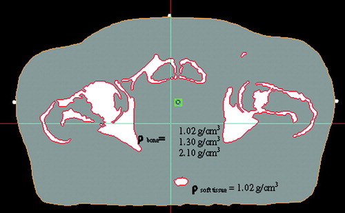
For each patient, four different image sets were created in the treatment planning system (TPS) Masterplan v.1.3 (Nucletron BV, Veenendahl, The Netherlands): (1) the original CT-series (CT_DP), (2) a simulated MR-series with all tissue set to a homogenous water equivalent material of density 1.02 g/cm³ (MR_W), (3) a simulated MR-series with soft tissue set to a water equivalent material of density 1.02 g/cm³ and the bone set to a density of 1.3 g/cm³ (MR_W + B1.3), and (4) a simulated MR-series identical to (3) but with a bone density equal to 2.1 g/cm³ (MR_W + B2.1). The tissue segmentation for MR-series (2)-(4) was carried out in the TPS by applying a semi-automatic Volume of Interest (VOI) extraction method based on a simple thresholding of image voxel values. All voxels with a Hounsfield number H < 156 were classified as water equivalent (ρ = 1.02 g/cm³), whereas voxels with H ≥ 156 were classified as bone (ρ = 1.02, 1.3 or 2.1 g/cm³). The densities were assigned separately to the two extracted regions (Figure 1). All image sets were stored in Masterplan as separate treatment cases. The bone density of 1.3 g/cm³ was selected as representative for a combination of cortical bone and trabecular bone and/or cartilage. The density of 2.1 g/cm³ (representative of compact bone) was selected to study the sensitivity of the calculated dose to an extreme choice of bone density.

Figure 1.  Simulated MR-image segmented into the two tissue classes soft tissue and bone. Soft tissue was assigned the water equivalent density of 1.02 g/cm³, whereas bone was assigned the densities 1.02 g/cm³ (water equivalent), 1.3 g/cm³ (mixture of cortical bone and trabecular bone/cartilage), and 2.1 g/cm³ (compact bone), respectively.

Four different volumes of interest (VOI) were delineated based on the original CT-series, CT_DP: The Clinical Target Volume (CTV), the external body contour, the urinary bladder and the rectum. Based on the CT_DP and the corresponding VOIs, 3D conformal treatment plans were constructed applying a four-field box technique containing one anterior beam, two opposed lateral beams as well as a posterior beam. One extra beam segment was added for each of the lateral beams to improve the dose homogeneity in the CTV. Multi leaf collimated treatment beams were automatically conformed to the beams-eye-view outline of the CTV applying an isotropic margin equal to 15 mm. The dose distribution was calculated using a collapsed cone based dose engine in Masterplan. The dose distributions based on CT_DP, DD_DP, were approved according to clinical acceptance criteria and procedures for EBRT of prostate cancer. The prescribed target dose of plans that were used in this study was 50 Gy, and the calculated dose distributions were normalised to give an average dose of 50 Gy in the CTV. Usually, these plans represent the first series of a treatment course that also contains a second boost series targeting the prostate only to give a total target dose of 74 Gy.

The clinically approved plans including the VOIs were copied to image sets (2)-(4) to give a total of four plans for each patient. The defined VOIs were in all cases classified as water equivalent tissue with a density of 1.02 g/cm³. Subsequently, the dose distributions were recalculated utilizing the monitor units of each beam from the original plan, to give three new dose distributions, DD _W, DD _W + B1.3, and DD _W + B2.1. These resulting dose distributions were compared to DD_DP by analysing dose-volume histograms (DVH), dose difference histograms (DDH) as well as through a visual display and inspection of voxel by voxel dose differences.

Evaluating the feasibility of sole MRI based planning

The results of the CT based simulation analysis were used as a basis for evaluating a strategy for the sole use of MR images for treatment planning. A patient referred to EBRT for prostate cancer was first CT scanned. Next, a standard 4-field box technique plan as well as a 7 field IMRT treatment plan (equidistant gantry angles) were designed and approved according to the clinical procedures and details outlined above. In addition, simulated MR images were created in a similar manner as for the ten cases described above. Immediately after the planning CT scan, the patient was scanned on a MR-simulator (MAGNETOM Espreee, 1.5 T, Siemens Medical Solutions USA, Inc.). The patient pose was made as similar as possible to that used during the CT scan. This included the use of a flat table top, application of a knee fix as well as the use of a radiotherapy dedicated laser system for correct set up of the patient w.r.t. to the skin tattoos. Axial, T2-weighted MR images were acquired using a single slab 3D turbo spin-echo pulse sequence (SPACE) with 1.3 mm isotropic resolution (TR 1500 ms, TE 150 ms, TA 9 min, slice thickness 1.3 mm, partitions 224, matrix 224×320, FOV 280×400 mm²). The MR images were post-processed to correct for image distortion caused by non-linearities in magnetic gradient field, using the 3D image distortion correction algorithm provided by the vendor.

To enable a direct comparison of CT and the MRI based dose calculations, the MR images were resampled to reflect the spatial dimensions of the CT data. This resulted in a MR image series containing 82 image slices of slice thickness and slice distance of 2.5 mm, respectively, and a spatial resolution of 0.98 mm in a 512×512 image matrix. Furthermore, the MR images were manually registered with the CT images using corresponding anatomical landmarks (e.g. bone surfaces). The latter enabled a direct transfer of the VOIs from the CT image series to the MR images.

In this context segmentation of the pelvic bone structures in the MR images was achieved by two different methods. The first approach was based on an in-house developed method for conversion of MR images into Hounsfield density maps that include an identification of cortical bone. First, MR images were processed to extract normalized exponentially enhanced grey value gradients. Gradient values larger than 0.1 were preliminary classified as bone. Next-this segmentation was refined utilizing an atlas like bone structure extracted from corresponding CT images in order to search for, and identify, those pixels that represent true cortical bone. Finally, the MR image values were mapped into Hounsfield like values by compressing soft tissue pixel values into the water equivalent range [−32,32] and the extracted cortical bone structures into the range [245,1145] with an average value typically of the order 450 (Figure 2). The latter would correspond to a bone tissue density in Masterplan of around 1.3 g/cm³. The tissue segmented MR images were imported into Masterplan, associated with the CT based treatment plan and corresponding VOIs, and finally a dose distribution, DD_MR, was calculated and the relevant dose statistics was attained.

Figure 2.  Hounsfield density mapped MR-image with segmented cortical bone. The segmented cortical bone was assigned values in the range of [245,1145] and soft tissue was compressed into the range [−32,32].

The second approach for MRI bone segmentation was a simple brute force manual contouring of the pelvic skeleton utilizing the extracted cortical bone by applying the structure drawing tool in Masterplan. As for the simulated MR images, soft tissue was assigned a water equivalent density of 1.02 g/cm³, whereas the VOI representing the skeleton was assigned densities equal to 1.02 g/cm³, 1.3 g/cm³ and 2.1 g/cm³ to produce the image series MR_W, MR_W + B1.3, MR_W + B2.1. Next, both of the the clinically approved CT based treatment plans were associated with each of these three images series, and the dose distributions DD^MR_W, DD^MR_{W + B1.3,} DD^MR_W + B2.1 were calculated.

Results

Figure 3 shows a typical example (patient no. 7) of the dose differences DD _DP-DD _W, DD _DP-DD _W + B1.3, and DD _DP-DD _W + B2.1 for all the voxels enclosed by the CTV. Table I summarizes the corresponding relative dose statistics for all of the ten patients in the study. The population based mean deviations in the mean CTV dose, i.e. the average absolute deviation relative to the prescribed dose, shows that both DD_W and DD_W + B1.3 only exhibit minor discrepancies when compared to the approved dose distribution, the differences were −0.9% (or −0.5 Gy) and 0.2% (or 0.1 Gy), respectively, whereas DD_W + B2.1 deviates by as much as 4.2% (or 2.1 Gy). The population based mean deviation for the minimum CTV dose was −2.75% (or −1.33 Gy), −1.6% (or −0.8 Gy) and −4.3% (or −2.1 Gy) for DD_W, DD_W + B1.3 and DD_W + B2.1 respectively, i.e. when using the simulated MR images the minimum CTV dose was slightly overestimated.

Figure 3.  Histogram of the absolute dose differences DD_DP-DD_W (2), DD_DP-DD_W + B1.3(3), and DD_DP-DD_W + B2.1 (4) for all voxels enclosed in the CTV (patient no. 7).

Figure 4.  Histogram of the absolute dose differences DD_DP-DD_W + B1.3(1), DD_DP -DD^MR_W + B1.3 (2) and DD_DP-DD_MR (3) for all voxels enclosed in the CTV for the patient who underwent both a planning CT scan and a MRI scan.

Table I.  Dose statistics for the CTV, bladder and rectum that shows the relative differences between clinically approved dose distribution (DD_DP) and the dose distributions based upon simulated MR images, DD_W, DD_W + B1.3, DD_W + B2.1 (refer to text for details). Prescribed target dose was 50 Gy.

	CTV							Bladder				Rectum
	Volume [cm^3]	Rel. diff. min. dose [%]			Rel. diff. mean. dose [%]			Volume [cm^3]	Rel. diff. max. dose [%]			Volume [cm^3]	Rel. diff. max. dose
Pat. no.		DDW	DDW + B1.3	DDW + B2.1	DDW	DDW + B1.3	DDW + B2.1		DDW	DDW + B1.3	DDW + B2.1		DDW	DDW + B1.3	DDW + B2.1
1	88.0	−2.2	−1.1	−5.2	−1.0	0.5	5.8	64.2	3.8	3.9	7.5	84.9	4.2	4.9	8.5
2	123.0	−2.7	−2.0	−3.0	−0.7	0.0	2.5	219.8	9.6	9.6	9.5	53.7	7.2	7.4	8.6
3	141.2	−2.4	−1.6	−4.6	−0.9	0.2	4.2	127.2	7.0	7.2	8.6	88.6	5.9	6.2	8.1
4	139.7	−3.4	−2.0	−5.6	−1.2	0.2	4.9	113.2	1.5	1.9	8.8	94.8	5.8	6.3	8.3
5	146.2	−2.0	−1.4	−5.3	−0.7	0.2	3.6	72.1	3.3	3.4	4.6	78.9	5.5	6.9	12.2
6	125.9	−2.7	−1.6	−3.3	−0.7	0.2	3.4	88.5	3.4	3.6	4.7	122.3	4.6	5.3	9.3
7	99.8	−3.1	−1.8	−4.1	−1.3	0.1	5.5	232.0	2.2	2.2	11.0	64.2	4.3	5.0	9.7
8	107.1	−3.4	−1.5	−0.4	−0.8	0.3	4.4	58.6	2.5	2.6	5.2	56.6	−3.6	2.6	5.1
9	185.5	−3.4	−2.2	−5.4	−1.1	0.2	5.2	54.8	2.5	2.4	5.0	76.2	2.4	2.4	9.0
10	185.0	−2.4	−1.2	−6.3	−0.8	0.0	2.9	61.8	4.4	4.4	5.2	60.5	5.2	5.9	8.9
Avg.	134.1	−2.8	−1.6	−4.3	−0.9	0.2	4.2	109.2	4.0	4.1	7.0	78.0	4.2	5.3	8.8
Std.dev.		0.5	0.4	1.7	0.2	0.2	1.1		2.5	2.5	2.3	21.0	3.0	1.7	1.8
Population based mean		−2.7	−1.6	−4.3	−0.9	0.2	4.2		4.0	4.1	7.0		4.2	5.3	8.8

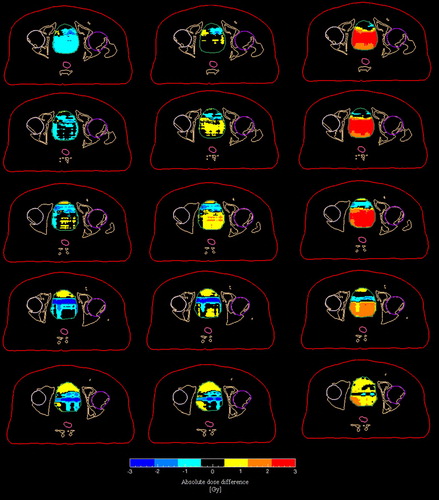
The population based mean deviations for the mean bladder dose (Table I) from the clinically accepted dose were −0.6% (or −0.25 Gy), 0.1% (or 0.0 Gy), and 2.5% (or 1.1 Gy) for the DD_W, DD_W + B1.3 and DD_W + B2.1 respectively. The corresponding values for the maximum doses were 4.1% (or 2.1 Gy), 4.1% (or 2.1 Gy) and 7.1% (or 3.6 Gy), i.e. applying the simulated MR images resulted in an underestimation of the maximum bladder doses. Figure 5 illustrates the spatial variation of the absolute dose differences across the entire bladder for patient number 7.

Figure 5.  Absolute dose difference maps of the bladder for five axial slices (patient no. 7) in the simulated MR series. From left to right, the following differences are shown: DD_DP-DD_W, DD_DP-DD_W + B1.3 and DD_DP-DD_W + B2.1

The population based mean deviations (Table I) for the mean rectum dose from the clinically accepted dose were −0.7% (or −0.25 Gy), 0.1% (or 0.0 Gy), and 0.8% (or 1.1 Gy) for the DD_W, DD_W + B1.3 and DD_W + B2.1 respectively. The corresponding values for the maximum doses were 4.1% (or 2.1 Gy), 5.3% (or 2.7 Gy) and 8.8% (or 4.5 Gy), i.e. applying the simulated MR images resulted in an underestimation of the maximum rectum doses.

Table II summarizes the absolute dose statistics for the patient case where a dose distribution was calculated from the planning CT images, simulated MR and true MR images. The rows marked 4F Box CC refers to the 4-field box plan, whereas the rows marked IMRT refers to 7-field IMRT plan. The rows indexed with simMR give the difference between the clinically approved dose distribution and the dose distributions based on the simulated MR images for this patient case. The rows indexed trueMR refer to the difference between the clinically approved dose plan and the dose distribution derived from the actual MR images acquired for this patient. When using the tissue segmented MR images created by the in-house developed bone segmentation method, only minor differences in mean CTV dose from the clinically approved dose plans were observed; −0.3 and 0.0 Gy for the 4-field box and IMRT plan, respectively. Corresponding values for the minimum CTV dose were −0.8 Gy and −0.4 Gy, respectively. Figure 4 shows the corresponding histogram of the 4-field box plan for the dose differences DD_DP−DD_W + B1.3(1), DD_DP−DD^MR_W + B1.3(2), and DD_DP−DD_MR(3) for all the voxels enclosed by the CTV. The corresponding histogram for the IMRT plan was very similar. For the organs at risk, the deviations are somewhat larger, but of the same order as the results derived from the simulated MR images.

Table II.  Dose statistics for treatment plans created for the case where both simulated MR images as well as true MR images were used as planning basis (refer to text for details). The rows indexed simMR show the absolute differences between the clinically approved dose distribution (DD_DP) and the dose distributions based upon the simulated MR images. The rows indexed trueMR show the absolute differences between the clinically approved dose distribution (DD_DP) and the dose distributions based upon the true MR images (DD_MR). The statistics for a standard 4-field box technique plan (4 F Box CC) as well as for a 7 beam IMRT plan is shown.

VOI	Volume [cm^3]			Min. abs. dose diff. [Gy]				Max. abs. dose diff. [Gy]				Mean. abs. dose diff. [Gy]
				DDW	DDW + B1.3	DDW + B2.1	DDMR	DDW	DDW + B1.3	DDW + B2.1	DDMR	DDW	DDW + B1.3	DDW + B2.1	DDMR
CTV	45.9	4 F Box	simMR	−1.18	−0.61	−2.4	–	0.19	0.55	3.5	–	−0.53	−0.05	1.63	–
			trueMR	−1.12	−0.65	−3.22	−0.78	0.23	1.09	6.4	1.22	−0.57	0.48	4.01	−0.29
		IMRT	simMR	−0.82	−0.33	0.38	–	0.21	0.48	2.16	–	−0.33	0.07	1.18	–
			trueMR	−0.69	−0.04	1.00	−0.36	0.39	1.04	3.97	0.63	−0.23	0.47	2.30	0.04
Bladder	54.5	4 F Box	simMR	−2.14	−1.97	−2.07	–	2.18	2.48	4.01	–	−0.35	0.15	1.95	–
			trueMR	−1.79	−1.38	−1.52	−2.05	0.96	1.37	6.58	1.01	−0.27	0.62	3.65	−0.17
		IMRT	simMR	−0.63	−0.18	−0.06	–	0.20	0.45	2.36	–	−0.20	0.10	0.93	–
			trueMR	−0.50	−0.07	−0.05	−0.20	0.30	1.17	4.23	0.58	−0.05	0.56	2.16	0.20
Rectum	88.2	4 F Box	simMR	−3.01	−2.76	−1.86	–	3.31	3.42	3.84	–	−0.29	0.02	1.19	–
			trueMR	−2.96	−2.52	−1.48	−3.18	2.78	3.03	6.08	2.86	−0.2	0.46	2.89	0.09
		IMRT	simMR	−0.50	−0.28	−0.18	–	0.61	0.88	1.74	–	−0.02	0.15	0.62	–
			trueMR	−0.44	−0.22	−0.03	−0.30	0.93	1.54	3.20	1.25	0.06	0.35	1.13	0.21

Discussion

The current work shows that a limited tissue segmentation of MR images may be appropriate to obtain an adequate dose as well as dose distribution across the CTV for EBRT of prostate cancer. It should be emphasised that this result only applies to the given treatment technique studied and with reference to the relevant clinical acceptance criteria for this type of treatment in our clinic. By classifying the pelvic tissue as water equivalent soft tissue and bone tissue of density 1.3 g/cm³, an average dose deviation of only 0.2% from the clinically approved dose plan was attained based on simulated MR images. Even when applying no segmentation, i.e. by classifying all tissue as water equivalent, a discrepancy of no more than −1% was found. Likewise, the minimum CTV dose deviates by −1.6% only.

From Table II it is seen that the dose differences for plans based on the simulated MR images for this particular patient were of the same order of magnitude as the results presented in Table I, i.e. this patient may be considered as representative for this specific patient group. In addition, the use of a more sophisticated IMRT based treatment technique did not make any difference with respect to which tissue classification strategy to use, i.e. water and bone with density 1.3 g/cm³ gave the best agreement with the clinically approved plan. It can also be noted that the discrepancies between (DD_DP-DD_W + 1.3) and (DD_DP-DD_MR), irrespective of treatment technique, were of the order <0.5 Gy. In other words, the findings of the simulation study, i.e. that bone should be extracted to achieve an acceptable dose distribution, holds also for the use of true MR images. This conclusion is further substantiated by looking at discrepancies observed for the plans based on the actual tissue segmented MR images, DD_MR. These may from a clinical point of view, be regarded as negligible. Typically the discrepancies for the mean CTV dose were less than 0.5 Gy, the discrepancies for the maximum dose to bladder as well as the minimum CTV dose were of the order <1 Gy, and the maximum dose to the rectum is of the order 3 Gy and 0.5 Gy for the 4-field and IMRT plans, respectively.

However, the segmentation of the bone structures from the MR images is in general a very complex problem, and a separate project in the department is dedicated to this topic. In the simulated MR images, bone structures were extracted purely on the basis of a fixed Hounsfield unit threshold (H > 156). As one can see from Figure 1 this typically leads to a classification of trabecular bone as soft tissue. By assigning a tissue density of 1.3 g/cm³ to the remaining structure that was extracted in this manner, an excellent agreement with the CTV dose of the actual treatment plan was attained. This indicates that a classification of trabecular bone as soft tissue and the use of 1.3 g/cm³ as bone density is sufficient. However, the dose distribution derived from brute force contouring of the skeleton in true MR images, and subsequently assigning a density of 1.3 g/cm³ to the resulting VOI, resulted in an underestimation of the mean CTV dose (Table II and histogram (2) in Figure 4). This indicates that when contouring the entire skeleton, a slightly lower density than 1.3 g/cm³ could be appropriate as proposed by Lee et al. [8]. The in-house developed segmentation procedure that only extracts cortical bone gives similar deviations, but of opposite sign (see Table II and histogram (3) in Figure 4). This means that a mere extraction of cortical bone is not sufficient in order to produce an adequate attenuation of the radiation and results in an overestimation of the mean CTV dose.

From Table I it is seen that setting the bone density to 2.1 g/cm³ significantly increases the dose inhomogeneity in the CTV, as well as leading to deviations from the clinically approved plans in all aspects. Even though a density of 2.1 g/cm³ is representative for some bony details, applying this density will definitely lead to an overestimation of the attenuation that takes place in the bone tissue in the pelvic region. The results also show that the maximum doses in the organs at risk can be underestimated by typically 4% if limited tissue segmentation is performed. This indicates that one should be very careful in scoring late effects for serially oriented organs based on the dose distributions generated from such images.

This study did not address the effect of non-linearities in the main magnetic and gradient fields that may give rise to geometrical inaccuracies in the MR images. A characterisation of such non-linearities for the MR machine used in this study is the topic of another project in the department [14]. Preliminary tests performed in-house indicate that these effects will be minor compared to the daily variation in the external body contour as long as the vendor supplied 3D image distortion correction algorithm is applied. Declaration of interest: The authors report no conflicts of interest. The authors alone are responsible for the content and writing of the paper.

References

- Debois M, Oyen R, Maes F, Verswijvel G, Gatti G, Bosmans H, et al. The contribution of magnetic resonance imaging to the three-dimensional treatment planning of localized prostate cancer. Int J Radiat Oncol Biol Phys 1999; 45: 857–65
- Rasch C, Barillot I, Remeijer P, Touw A, van Herk M, Lebesque JV. Definition of the prostate in CT and MRI: A multi-observer study. Int J Radiat Oncol Biol Phys 1999; 43: 57–66
- Khoo VS, Padhani AR, Tanner SF, Finnigan DJ, Leach MO, Dearnaley DP. Comparison of MRI with CT for the radiotherapy planning of prostate cancer: A feasibility study. Br J Radiol 1999; 72: 590–7
- Sannazzari GL, Ragona R, Redda MG, Giglioli FR, Isolato G, Guarneri A. CT-MRI image fusion for delineation of volumes in three-dimensional conformal radiation therapy in the treatment of localized prostate cancer. Br J Radiol 2002; 75: 603–7
- Chen L, Nguyen TB, Jones É, Chen Z, Luo W, Wang L, et al. Magnetic resonance-based treatment planning for prostate intensity-modulated radiotherapy: Creation of digitally reconstructed radiographs. Int J Radiat Oncol Biol Phys 2007; 68: 903–11
- Chen L, PriceJr RA, Nguyen T-B, Wang L, Li JS, Qin L, et al. Dosimetric evaluation of MRI-based treatment planning for prostate cancer. Phys Med Biol 2004; 49: 5157–70
- Chen L, PriceJr RA, Wang L, Jinsheng L, Qin L, Shawn M, et al. MRI-based treatment planning for radiotherapy: Dosimetric verification for prostate IMRT. Int J Radiat Oncol Biol Phys 2004; 60: 636–47
- Lee YK, Bollet M, Charles-Edwards G, Flower MA, Leach MO, McNair H, et al. Radiotherapy treatment planning of prostate cancer using magnetic resonance imaging alone. Radiother Oncol 2003; 66: 203–16
- Kristensen BH, Laursen FJ, Løgager V, Geertsen PF, Krarup-Hansen A. Dosimetric and geometric evaluation of an open low-field magnetic resonance simulator for radiotherapy treatment planning of brain tumors. Radiother Oncol 2008; 87: 100–9
- Prabhakar R., Julka PK, Ganesh T, Munshi A, Joshi RC, Rath GK. Feasibility of using MRI alone for 3D radiation treatment planning in brain tumors. Jpn J Clin Oncol 2007; 37: 405–11
- Beavis AW, Gibbs P, Dealey RA, Whitton VJ. Radiotherapy treatment planning of brain tumors using MRI alone. Br J Radiol 1998;544–8.
- Khoo VS, Dearnaley DP, Finnigan DJ, Padhani A, Tanner SF, Leach MO. Magnetic resonance imaging (MRI): Considerations and applications in radiotherapy treatment planning. Radiol Oncol 1997; 42: 1–15
- Fransson A, Andreo P, Pötter R. Aspects of MR image distortions in radiotherapy treatment planning. Strahlenther Onkol 2001; 177: 59–73
- Vestad TA, Geier OM, Eilertsen K, Skretting A. Evaluation of geometrical accuracy in magnetic resonance imaging by means of a phantom tailored for automatic computer analysis. 2008 ( submitted).