Abstract
Background. Treating small tumours in the brain requires usage of small fields. However, it is a challenge for all treatment planning systems (TPS) to modulate small fields (≤3×3 cm2) for which lateral electronic equilibrium does not exits. Material and methods. Open field beam data was measured for the stereotactic mode at our Varian Trilogy accelerator and was implemented in the Eclipse TPS for both the Pencil Beam (PB) and the Anisotropic Analytical Algorithm (AAA). Additional output factors, profiles and percentage depth dose curves were measured in a water phantom for asymmetric fields and fields defined by the Varian 120 MLC and the BrainLAB m3 MLC. Dose distributions in transverse sections were measured with gafchromic films in a homogeneous phantom. These were compared to those calculated by the Eclipse TPS for 11 stereotactic treatment plans. The plans included non-coplanar, dynamic and arc fields. All comparisons for the film measurements in the phantom were made with a Gamma criterion of 2 mm in distance and 3% in dose. Results. The AAA and the PB algorithms broadened the penumbra of the profiles by approximately 1.5 mm and 2.0 mm, respectively. For static fields defined by the Varian 120 MLC, the measured field size was 1.0 mm broader than the calculated. The output factors were typically within 2% for field sizes ≥ 2×2 cm2. More than 95% of the points passed the Gamma criterion. Up to 50% of the points in the low dose regions failed the criterion, but overall the match was satisfactory. Conclusion. The accuracy of calculations performed by the Eclipse TPS for the SRS mode was shown to be within a few percent for most clinical fields. AAA was found to be superior to the PB algorithm in modelling the dose in the penumbra region.
Small tumours (typically below 3×3 cm2) in the brain are often treated by Stereotactic Radio Surgery (SRS) where the patient is fixated very precisely and a high dose (approximately 20 Gy) is delivered in one or a few fractions. For stereotactic treatment in the brain, very complex treatment plans are often necessary in order to cover the target sufficiently and avoid damage to the organs at risk. These plans may include Intensity Modulated RadioTherapy (IMRT) and/or several non-coplanar fields.
Measurement and calculation of small fields (less than 3×3 cm2) is complicated as lateral electronic equilibrium do not exist even at the central axis Citation[1]. The detectors used to measure the input parameters in the TPS should be carefully chosen in order to produce reliable results. For the TPS a variety of different calculation algorithms exist, varying from very simple algorithms to Monte Carlo based algorithms, which accounts accurately for lateral electron transport.
In the present study, the accuracy of a pencil beam (PB) algorithm Citation[2–4] and a convolution based (Anisotropic Analytical Algorithm, AAA) algorithm accounting in an approximate way for lateral scatter Citation[5–7] has been studied for a new SRS flattening filter. A variety of field configurations vere examined. Corresponding tests of the AAA and PB algorithms have been performed in homogeneous and inhomogeneous media for the standard Millenium flattening filter Citation[8–10]. These tests only include field sizes ≥ 3×3 cm2. In the present work, field sizes from 1×1 cm2 to 15×15 cm2, appropriate for stereotactic treatment of brain tumours, have been investigated for the SRS flattening filter. The objective was to examine the accuracy of the algorithms in homogeneous media for simple as well as complicated field configurations. The investigated fields were defined either by the jaws of the accelerator, the Varian Millenium 120 MLC, or the m3 MLC delivered by BrainLAB. Special attention was paid to the modelling of the field size and penumbra region, as a very precise modelling of the dose at the field edge is required for stereotactic treatments. Additionally, the accuracy of the algorithms was tested in two dimensions for several clinical plans.
Material and methods
Equipment and beam data
The measurements were performed on our Varian Trilogy linear accelerator which was able to deliver 6 MV photons with a dose rate of 1000 MU/min, when the SRS flattening filter was selected. The SRS flattening filter supports field sizes up to 15×15 cm2. This study focused on the SRS mode only.
The accelerator (Varian Medical systems, USA) was equipped with a Varian Millenium 120 MLC with a 5 mm leaf width centrally. It was possible to mount a BrainLAB (BrainLAB, Germany) m3 MLC. For this MLC the width of the leaves is 3 mm. When the m3 MLC is mounted on the accelerator head, the Millenium MLC is retracted and not in use.
We used Eclipse version 8.050 (Varian Medical systems, USA) for this study, and both the PB and the AAA algorithm was implemented in this TPS. These two algorithms require beam profiles, depth dose curves and an output factor table measured in a water phantom for square fields in the range from 1×1 cm2 to 15×15 cm2. The profiles were measured in the x direction for five specified depths. Only profiles measured in one direction may be introduced in the TPS. All fields were defined by the jaws of the accelerator. No additional profiles were required for fields defined by an MLC.
Depth dose curves and profiles were measured with a Source Surface Distance (SSD) equal to 100 cm in a water phantom (model MP3, PTW, Germany); this was denoted the reference configuration. Output factors were measured with a SSD = 95 cm and at a depth of 5 cm in the water phantom.
The profiles and the output factors were measured with the diamond detector of PTW in a horizontal position. The depth dose curves were measured with the diamond detector in a vertical position. The depth dose curves were compared to measurements made with a Rune Karlson (RK) ion chamber (Precitron, Sweden). These measurements were used to correct the depth dose curves for the dose rate dependence of the diamond detector Citation[11].
The SRS mode does not include the possibility to configure dynamic wedges.
Finally, for the dynamic treatment the transmission through the leaves and the dosimetric leaf separation, which models the leakage through the rounded leaf tips, were determined.
The grid size for all calculations was set to 2.5 mm. This was chosen because it was the smallest identical grid size to be chosen for the two algorithms. A few measurements were performed as a check with the smallest available grid size, being 1.25 mm for PB and 2.0 mm for AAA.
Fields defined by the jaws of the accelerator
After the configuration of the PB and AAA algorithms, an analysis of the calculated versus the measured beam data was performed for selected depth dose curves, profiles and output factors used for the configuration of the algorithms. For the PB algorithm, the measured and calculated depth dose curves are identical for SSD = 100 cm, as this algorithm uses the experimental curves.
Additional depth dose curves, profiles and output factors were measured to test the performance of the algorithms in the water phantom using the diamond detector. Selected profiles were measured in the y direction for depths of d = dmax, 5 cm and 10 cm in the reference configuration.
Profiles, depth dose curves and output factors were measured with d = dmax, 5 cm and 10 cm for SSD = 90 cm and field sizes of 2×2, 5×5 and 10×10 cm2. Output factors were also measured for SSD = 100 cm.
Profiles were measured at a depth of d = 5 cm for five asymmetric fields in the direction of asymmetry, see . Four of the fields were created with overtravel of one jaw in the y direction. One field was made with overtravel in the x direction. Depth dose curves were measured centrally in the field for all five asymmetric fields. Output factors were measured centrally for ten asymmetric fields including those mentioned above.
Table I. Asymmetric fields.
Fields defined by the MLC
Profiles were measured at d = 5 cm and SSD = 100 cm in the water phantom for field sizes of 1×1, 2×2 and 5×5 cm2 defined by either the Millenium 120 MLC or the m3 MLC. The scans were performed both in the direction parallel and perpendicular to the direction of leaf motion. In the direction perpendicular to the leaf motion, closed leaf pairs were offset from the central axis of the field. In the direction parallel to the leaf motion, profiles were measured on the central axis of the field and at the position of half the leaf width (2.5 mm for the Millenium 120 MLC, 1.5 mm for the m3 MLC). The profiles measured on the central axis and at the position of half the leaf width were identical. This was also true for the calculated profiles.
Depth dose curves were measured centrally for these fields.
Output factors were measured centrally for symmetrical fields defined by both MLCs with field sizes of 1×1, 2×2, 3×3, 5×5 and 10×10 cm2. The jaws defined the equivalent field size or larger field sizes. For instance, output factors were measured for the 1×1 cm2 field defined by the MLC with the jaws defining fields of 1×1, 2×2, 3×3 and 5×5 cm2. In addition, output factors were measured centrally for 14 selected rectangular fields defined by the m3 MLC with the jaws defining a slightly larger field. For instance a 1.2×5 cm2 field with the jaws at x = 2 and y = 6.
Treatment plans
The IMRT verification head/neck phantom (model T40015) from PTW (PTW, Germany) was scanned and 11 treatment plans were created. We mounted radiographic films in the sliced part of the phantom. Moreover, a cylindrical detector was inserted on the central axis. The treatment plans were created in order to test a variety of configurations. The plans included very small (1.5×1.5 cm2) fields, asymmetric fields, non-coplanar fields, intensity modulated fields and dynamic arc fields. The plans are described in where also the slices in the phantom selected for film measurements are listed. All plans were calculated with both algorithms. Moreover, nearly identical plans have been calculated and tested for both MLCs. All plans were created with an isocenter dose between 3 and 4 Gy.
Table II. Nomenclature and description of treatment plans
The dose at the isocentre was measured with the diamond detector for each treatment plan.
Gafchromic EBT films (ISP, USA) were mounted in the phantom parallel to the beam axis (for a gantry angle of zero) and the phantom was irradiated with the treatment plans one at a time. The dose distribution in the selected transversal planes inside the phantom where calculated by Eclipse using the PB and AAA algorithms and exported to Verisoft (PTW, Germany) for a comparison to the dose distribution measured with the film.
The calibration of the film was performed with three separate films irradiated with known doses from 1 to 4 Gy. The films were mounted between 20 cm of box shaped solid water (Gammex, USA) parallel to the beam. Irradiation in this position gave rise to a depth dose curve and the calibration curve was determined from a comparison of points on this curve to the similar points determined by Eclipse.
All films were evaluated with a Gamma criterion Citation[12] of 3% in local dose and 2 mm in Distance To Agreement (DTA).
Results
Fields defined by the jaws of the accelerator
The calculated depth doses agreed with measurements within 1.5% and 2 mm for all points for the AAA algorithm, apart from the field size of 1×1 cm2. After dmax the agreement was within 0.5%. For the field size of 1×1 cm2, deviations up to 4% were observed. AAA showed a tendency to slightly underestimate the dose after dmax for small field sizes and slightly overestimate the dose for large field sizes.
The AAA algorithm showed a slightly better overall agreement in all parts of the profiles than the PB algorithm. Especially in the low dose region below the jaws, AAA was superior to the PB algorithm, see . Both algorithms overestimated the width of the penumbra region (defined as the region where the dose changes from 80 to 20%). AAA broadened the penumbra by approximately 1.5 mm almost independent of field size and depth. PB broadened the penumbra by approximately 2.0 mm. These numbers were unaffected by the grid size being 2.5 mm or less. The penumbras of the profiles measured in the y direction were approximately 0.2 mm broader than those measured in the x direction. The calculated profiles were identical in the two directions.
Figure 1. Profiles measured and calculated for SSD = 100 cm with a depth d = 5 cm. Field sizes of 2×2 cm2 and 5×5 cm2. The curves shown are: (——) measured curve, (grey——) AAA, and (- - - -) PB calculation. The dose values are normalized to the central axis dose.
For AAA, a maximum deviation of 0.4% for all fields was found for output factors measured at SSD = 95 cm, except for the field size of 1×1 cm2 which showed a deviation of 1%. The PB algorithm showed deviations up to 3% for field sizes with x or y equal to 1. For all other field sizes the maximum deviation was below 0.4%.
Comparison of measured profiles and depth dose curves for SSD = 90 cm to calculations performed with the AAA and PB algorithms showed results very similar to those obtained in the reference condition. Output factors measured and calculated centrally in the field for SSD = 90 and 100 cm showed deviations below 1% for all field sizes with x and y ≥ 2 cm for both algorithms.
The agreement of the measured and calculated profiles of the asymmetric fields was very similar to the findings for the symmetric fields. The penumbra was broader for both algorithms but AAA performed better than the PB algorithm. For the depth dose curves, the calculated depth doses for AAA agreed within 2% and 2 mm below dmax except for the extreme field y5,7 where the y jaw overtravels the axis by 5 cm. Here larger deviations were seen for depths larger than 10 cm, see . The PB algorithm showed larger deviations and especially calculated depth doses of the field y5,7 deviated substantially as seen in . The fields with overtravel of 1 cm in x or y direction showed deviations below 2% and 2 mm. For the AAA algorithm, the maximum deviation of the output factors of the asymmetric fields was 0.8%, whereas the PB algorithm underestimated the dose with up to 4%.
Figure 2. Depth dose curves measured and calculated for SSD = 100 cm for the asymmetric field denoted y5,7. The curves shown are: (——) measured curve, (grey——) AAA, and (- - - -) PB calculation. The dose values are normalized to dmax.
Fields defined by the MLC
In measured and calculated profiles in the direction of leaf motion are shown for a 2×2 cm2 field collimated by the Millenium 120 MLC. The measured field size was larger than the calculated by approximately 2 mm. The profile of the 2×2 cm2 field collimated by the MLC was slightly better modelled by the AAA than the PB algorithm. Both algorithms broadened the penumbra by the same order of magnitude as for fields defined by the jaws. In the direction perpendicular to the leaf motion, there was a good correlation between the measured and calculated profiles for fields defined by the MLC, except for the broadening of the penumbra, see . The broadening was of the same order of magnitude as for the fields defined by the jaws. Similar results were found for 1×1 cm2 and 5×5 cm2 fields.
Figure 3. Profiles measured and calculated for SSD = 100 cm with d = 5 cm. Field size 2×2 cm2. The field is collimated by the Millenium 120 MLC. The profiles are measured in the direction parallel to the leaf motion. The curves shown are: (——) measured curve, (grey——) AAA and (- - - -) PB calculation. The dose values are normalized to the central axis dose.
Figure 4. Profiles measured and calculated for SSD = 100 cm with d = 5 cm. Field size 2×2 cm2. The field is collimated by the Millenium 120 MLC. The profiles are measured in the direction perpendicular to the leaf motion. The curves shown are: (——) measured curve, (grey——) AAA and (- - - -) PB calculation. The dose values are normalized to the central axis dose.
Measured and calculated depth dose curves did not depend on the collimator device being jaws or MLC.
All calculated output factors for the Millenium 120 MLC deviated from the measured output factors by less than 2% for both algorithms, except for the field size of 1×1 cm2. The PB algorithm overestimated the output factors, while AAA underestimated the output factors. For the 1×1 cm2 MLC defined field, PB overestimated the output factor by 8% when the jaws defined a 5×5 cm2 field. The AAA underestimated the output factor for this field by 6%.
Profiles measured in the direction of leaf motion are shown in for a 1.8×2 cm2 field defined by the m3 MLC and the jaws. The measured field size was approximately 1 mm larger than the calculated field size. The measured width of the penumbra was approximately 0.5 mm smaller than for the field defined by the jaws. The AAA algorithm modelled the measured profiles slightly better than the PB algorithm. Similar profiles were measured and calculated in the direction perpendicular to the leaf motion. In this direction no broadening of the field size was observed. Apart from this, the findings resemble those in the direction parallel to the leaf motion.
Figure 5. Profiles measured and calculated for SSD = 100 cm with d = 5 cm. Field size 2×2 cm2. The field is collimated by the m3 MLC. The profiles are measured in the direction parallel to the leaf motion. The curves shown are: (——) measured curve, (grey——) AAA and (- - - -) PB calculation. The dose values are normalized to the central axis dose.
Output factors measured centrally for symmetric and asymmetric fields deviated less than 3% from the calculated values for both algorithms independently of the position of the jaws. However, the majority of the output factors deviated less than 1%. The only exception was the 1.2×1 cm2 field which showed larger deviations: Up to 5% underestimation for AAA and up to 8% overestimation for PB.
Treatment plans
In the calculated dose distributions in the transverse section at the isocentre of some of the treatment plans described in are shown together with the Gamma analysis for both algorithms. Slightly better results were obtained for the Gamma analysis for AAA than for PB. Similar results were found for the m3 MLC.
Figure 6. Upper row: calculated dose distribution in dose colour wash for the isocentre slice of five treatment plans. For clarity only doses above 0.2 Gy are shown. Lower rows: Gamma analysis of the treatment plans (middle row: AAA, bottom row: PB). The Gamma criterion is 2 mm in DTA and 3% in dose. a) the plan named “12 fields”, b) the plan “3 arcs”, c) the plan “7 fields IMRT”, d) the plan “6 fields 1”, e) the plan “6 fields 5”. Red means that the Gamma criterion is not fulfilled. Green means that it is fulfilled.
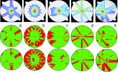
In a the gamma analysis of the plan named “12 fields” is shown. A good correlation was obtained for the majority of the points. The Gamma criterion only failed in the low dose region, where the dose was below 0.2 Gy. The maximum deviation was 10% which was 0.02 Gy. Eclipse underestimated the dose in these regions. Similar findings were obtained in the plane 1 cm caudal to the isocentre. The maximum dose in the plane 2 cm caudal to the isocentre was 0.8 Gy. Deviations up to 8% were seen centrally for the field and Eclipse overestimated the dose for all points in this region.
The plan named “3 arcs” is shown in b. Again a good correlation was obtained for the majority of the points. A disagreement was only seen in the low dose area, where the dose was below 0.3 Gy. Eclipse underestimated the dose by up to 20%. For the PB calculation the Gamma criterion was not fulfilled centrally, where Eclipse underestimated the dose by slightly more than 3%.
Intensity modulated fields were tested in the plan “7 fields IMRT” which is seen in c. The correlation was good, except for the low dose areas where the dose deviated up to 10%.
Very small fields were tested in the “plan 6 fields 1” (see d). The deviation between the calculated and the measured dose in the isocentre was 9% and centrally in the field it was 5% for the AAA algorithm. For the PB algorithm, the deviation in the isocentre was 4% and there was no deviation centrally in the field. Furthermore, Eclipse underestimated the dose in the low dose region by up to 20%.
Finally, asymmetric fields were contained in the plan “6 fields 5” shown in e. Once again the correlation was good for most of the points. Deviations up to 7% were seen for doses below 0.4 Gy for the AAA calculation. The Gamma criterion failed in a larger number of points for the PB algorithm. However, the points in the high dose area passed the criteria.
The results of the Gamma analysis of the treatment plans not shown in were similar to the plans discussed. More than 95% of the points in the high dose areas fulfilled the Gamma criterion, whereas larger deviations were seen in areas where the dose level was below approximately 0.3 Gy. In these areas Eclipse always underestimated the dose.
Point dose measurements were performed by the diamond detector in the isocentre for all treatment plans except the plan “6 fields 5”. The point dose measurements agreed with the film measurements within 1% for all treatment plans.
Discussion
In the present study it was found that both the AAA and the PB algorithms reproduced the measured data well in the standard configuration for field sizes from 1×1 cm2 to 15×15 cm2 tested for the SRS flattening filter. The results presented here are very similar to the results presented by van Esch et al. Citation[9] and Bragg et al. Citation[10] for field sizes ≥ 3×3 cm2 for the standard Millenium flattening filter of the 6 MV Varian Clinac 2100 C/D.
The penumbra of the profiles measured in the y direction was found to be approximately 0.2 mm broader than what was measured in the x direction. This is due to the configuration of the accelerator head, where the x jaws are closer to the phantom target than the y jaws. This effect has not been taken into account in the calculation model and the calculated profiles are identical in the two directions. Likewise, the sharpening of the penumbra for fields defined by the m3 collimator being very close to the phantom has not been taken into account.
The tests performed in this work included measurements for different SSDs, asymmetric fields and fields defined by the Millenium 120 MLC and the m3 MLC. For all these cases, the two algorithms performed quite similar and showed small deviations. However, in most cases the AAA was superior to the PB algorithm. Both algorithms overestimated the width of the penumbra, with the AAA performing best. This was observed for all field configurations including fields defined by MLC. AAA modulated the tails of the profiles at the field edge very precisely, whereas the PB algorithm dramatically underestimated the dose in this region. Both algorithms overestimated the field size of static fields defined by an MLC. This discrepancy is due to the transmission through the rounded leaf tips of the MLC Citation[13]. The dosimetric leaf separation parameter models this phenomenon by shifting the leaves closer together. However, this parameter is not implemented for static fields, but for dynamic fields the effect is taken into account.
In a similar study the performance of the Monte Carlo based BEAMnrc code for the m3 MLC mounted at a Varian accelerator was investigated Citation[14]. This algorithm models the treatment head of the accelerator including the m3 MLC and no discrepancy in field size was found.
Output factors were in most cases predicted within 2% for the AAA, with larger deviations seen for the PB algorithm. Both algorithms showed the largest deviations for a 1×1 cm2 field. For this field, deviations up to 6 or 8% were seen when defined by an MLC for the AAA or PB algorithms, respectively. However, this field size is normally not clinically relevant. For 2×2 cm2 field size both algorithms performed well. Likewise, a good agreement was seen for intensity modulated fields.
Algorithms based on Monte Carlo calculations perform better for field sizes of 1×1 cm2. For these algorithms deviations below 3% are seen Citation[14–16]. These algorithms account for lateral scatter in a precise way by simulating the energy deposited for each of a huge number of particles in the phantom. The AAA algorithm only accounts for lateral scatter in an approximate way by modelling the lateral scatter due to photons and electrons in a plane perpendicular to the incident beamlet and thus, performing a superposition of the depth dependent component and the lateral scatter component.
The clinical treatment plans tested, showed that both algorithms performed well in cases with many treatment fields. In high dose regions the Gamma criterion of 3% and 2 mm in DTA was fulfilled for all treatment plans with field size ≥ 2×2 cm2. In regions where the dose was below approximately 0.3 Gy deviations up to 20% in local dose were seen. Eclipse always underestimated the dose in the low dose regions. In the cranio-caudal direction deviations up to ±7% centrally in the field were seen in the penumbra region. These deviations may be due to the sensitivity of the position of the film cranio-caudally as both positive and negative deviations were seen. Thus, these deviations may not be trusted.
Very small fields showed deviations larger than 3% in dose at the isocentre. This is in accordance with the point dose measurements. Thus, reliable dose calculations demands field sizes ≥ 2×2 cm2. If field sizes of 1×1 cm2 are needed deviations in dose of up to 9% may be expected.
For coplanar fields SSD is equal for all fields, whereas for non-coplanar fields different SSDs were tested, as the phantom is spherical at the one end. The Gamma criterion was also fulfilled for these plans.
Accurate dose calculation and field definition is of great importance Citation[17], Citation[18], especially for the stereotactic treatment of small tumours. Precise modelling of the penumbra and field size is very important for the estimation of the dose to organs at risk close to the target. Therefore, modelling of more narrow penumbras and accounting for the dosimetric leaf separation for static fields, would yield more precise dose calculations. Furthermore, it is important that the TPS calculates a correct absolute dose distribution for simple as well as very complex field configurations, which are often necessary for stereotactic treatment in the brain. This is seen to be fulfilled for both algorithms, with the AAA being superior to the PB algorithm. However, deviations up to 9% may be seen for field sizes ≤ 2×2 cm2. As both algorithms may easily be implemented in the Eclipse TPS it is advisable to use the AAA algorithm. Furthermore, the AAA algorithm is known to give more reliable results in inhomogeneous media than the PBC algorithm Citation[9], Citation[10], Citation[19]. The brain tissue is rather homogeneous. However, the density of the scull is very different from that of the brain. All tests included in this study were performed in the IMRT head/neck verification phantom which is a homogeneous phantom.
We have used a diamond detector to measure all input parameters for the TPS. The diamond detector has in several studies Citation[20–22] been found to be ideal for measurements of depth dose curves, dose profiles and output factors. The diamond detector is ideal for measurements where lateral electronic disequilibrium exists, as the detector is nearly tissue equivalent. Therefore, the detector acts identical to the surrounding tissue, in this case water or solid water in the Head/Neck phantom.
In conclusion, the accuracy of calculations performed by the Eclipse TPS for the high dose rate SRS mode was shown to be within a few percent for most clinical fields. This applied to static or dynamic fields collimated by jaws, the Millenium 120 MLC or the m3 MLC. Both the AAA and the PB algorithms overestimated the field size for static fields collimated by an MLC. The AAA algorithm was superior to the PB algorithm in calculating output factors, the size of the penumbra region and the dose in the region outside the field edge.
References
- Duggan DM, Coffey CW. Small photon field dosimetry for stereotactic radiosurgery. Med Dosim 1998; 23: 153–9
- Storchi P, Woudstra E. Calculation of the absorbed dose distribution due to irregularly shaped photon beams using pencil beam kernels derived from basic beam data. Phys Med Biol 1996; 41: 637–56
- Storchi PRM, van Battum LJ, Woudstra E. Calculation of a pencil beam kernel from measured photon beam data. Phys Med Biol 1999; 44: 2917–28
- Storchi P, Woudstra E. Calculation models for determining the absorbed dose in water phantoms in off-axis planes of rectangular fields of open and wedged photon beams. Phys Med Biol 1995; 40: 511–27
- Ulmer W, Harder D. A triple Gaussian pencil beam model for photon beam treatment planning. Z Med Phys 1995; 5: 25–30
- Ulmer W, Harder D. Applications of a triple Gaussian pencil beam model for photon beam treatment planning. Z Med Phys 1996; 6: 68–74
- Ulmer W, Pyyry J, Waissl W. A 3D photon superposition/convolution algorithm and its foundation on results of Monte Carlo calculations. Phys Med Biol 2005; 50: 1767–90
- Fogliata A, Nicolini G, Vanetti E, Clivio A, Cozzi L. Dosimetric validation of the anisotropic analytical algorithm for photon dose calculation: Fundamental characterization in water. Med Phys Biol 2006; 51: 1421–38
- Van Esch A, Tillikainen L, Pyykkonen J, Tenhunen M, Helminen H, Siljamäki S, et al. Testing of the analytical anisotropic algorithm for photon dose calculation. Med Phys 2006; 33: 4130–48
- Bragg CM, Conway J. Dosimetric verification of the anisotropic analytical algorithm for radiotherapy treatment planning. Radiother Oncol 2006; 81: 315–23
- Fovler JF. Solid state electrical conductivity dosimeters. Radiation Dosimetry. Attix FH, Roesch WC, New York: Academic Press; 1966.
- Low DA, Harms WB, Mutic S, Purdy JA. A technique for the quantitative evaluation of dose distributions. Med Phys 1998; 25: 656–61
- LoSasso T, Chui C, Ling CC. Physical and dosimetric aspects of a multileaf collimation system used in the dynamic mode for implementing intensity modulated radiotherapy. Med Phys 1998; 25: 1919–27
- Belec J, Patrocinio H, Verhagen F. Development of a Monte Carlo model for the Brainlab microMLC. Phys Med Biol 2005; 50: 787–99
- Crop F, Reynaert N, Pittomvils G, Paelinck L, De Gersem W. Phys Med Biol 2007;52:3275–90.
- Deng J, Guerrero T, Ma C-M, Nath R. Modelling 6 MV photon beams of a stereotactic radiosurgery system for Monte Carlo treatment planning. Phys Med Biol 2004; 49: 1689–704
- Knöös T, Wieslander E, Cozzi L, Brink C, Fogliata A, Albers D, et al. Comparison of dose calculation algorithms for treatment planning in external photon beam therapy for clinical situations. Phys Med Biol 2006; 51: 5785–807
- Brahme A, Chavaudra J, Landberg T. Accuracy requirements and quality assurance of external beam therapy with protons and electrons. Acta Oncol 1988; 27: S1–S76
- Breitman K, Rathee S, Newcomb C, Murray B, Robinson D, et al. Experimental validation of the Eclipse AAA algorithm. J Appl Clin Med Phys 2007; 8: 76–92
- Haryanto F, Fippel M, Laub W, Dohm O, Nüsslin F. Investigation of photon beam output factors for conformal radiation therapy – Monte Carlo simulations and measurements. Phys Med Biol 2002; 47: N133–N143
- Heydrian M, Hoban PW, Beddoe AH. A comparison of dosimetry techniques in stereotactic radiosurgery. Phys Med Biol 1996; 41: 93–110
- Laub WU. The volume effect of detectors in the dosimetry of small fields used in IMRT. Med Phys 2003; 30: 341–7